Cluster arc statistics

Abstract

We study the strong gravitational lensing properties of galaxy clusters obtained from N-body simulations with standard $\Lambda$CDM cosmology. We have used the $32$ most massive clusters from a simulation at various redshifts and ray-traced through the clusters to investigate the giant arcs statistics. We have investigated the prevalence of multiple arc system, by looking at the multiple arc fraction (defined in the paper) systematically in various clusters and we have found that $\sim 40-50\%$ of the clusters that produce giant arcs give multiple arcs, which agrees with the RCSii observations. We have also investigated the mass distributions that are efficient in lensing, discussed effects of source sizes and various other factors that are very important in the formation of giant arcs.

1. Introduction

Strong gravitational lensing has become an important tool in cosmology. Lensing by clusters greatly magnifies distant sources, allowing us to view otherwise hard to observe galaxies (see Metcalfe et al. Metcalfe (2003); Smail et al. Smail (2002); Blain et al. Blain (1999)). Giant arcs provide us a direct probe of the gravitational potential of the lens and may enable us to study the background cosmology itself (see Bartelmann et al. Bart1 (1998); Dalal et al. Dalal (2004); Macciò Maccio (2004); Meneghetti et al. Meneg3 (2004)).

This subject has received a great deal of attention lately because Bartelmann et al. Bart1 (1998) reported that the predicted number of giant arcs varies by orders of magnitude among different cosmological models and the observed instances of giant arcs greatly exceeded the number of giant arcs predicted for $\Lambda$CDM (which has been widely supported by other lines of evidence e.g., Perlmutter et al. Perlm (1999), Riess et al. Riess (1998), Spergel et al. Spergel (2003), and Tegmark, Zaldarriaga & Hamilton Tegmark (2001)). The potential discrepancy between observations and theory in this arena is particularly puzzling because the giant arcs are probing the matter distribution in clusters on relatively large scales and we believe that we understand the behavior of such dark matter dominated structures, on large scales, very well from N-body simulations. This apparent discrepancy has led to significant work on refining the expected number of giant arcs. Bartelmann et al. Bart2 (2003) and Meneghetti et al. 2003b have confirmed the lensing cross section predicted by Bartelmann et al. Bart1 (1998). Wambsganss et al. Wambs (2004) found that the lensing cross section is a strong function of the source redshift, making it possible to get the observed number of giant arcs using a broader range of source redshifts. William et al. Will (1999) and Dalal et al. Dalal (2004) have suggested that massive galaxies ($10^{12}\,h^{-1}M_{\odot}$ - $10^{13}\,h^{-1}M_{\odot}$) are needed at the center of most low redshift arc bearing clusters. Further, triaxiality seems to be contributing to the formation of giant arcs, as Oguri et al. Oguri (2003) found that analytical models of cluster lenses with triaxiality and a steeper central potential enhance the lensing cross section. This work shows that the prediction of cross sections from theory remains a non-trivial exercise. In addition, in all of this work the comparison of theory with flux and surface brightness limited observations has been difficult.

However the activity has served to highlight the power of giant arcs to probe cosmology and structure formation, and progress has been made in both theory and observation. The EMSS (Luppino et al. Luppino (1999)) and LCDCS (Zaritsky & Gonzalez Zarit (2003)) surveys have found that the arc frequency is $\sim 20\%$ for massive clusters. Recent results from the Red Cluster Sequence (RCS) cluster survey suggest a higher lensing frequency, while they also found that multiple arc systems appear with a probability of $\sim 40\%$. New results from the ROSAT Bright Survey Schwope (2000) analyzed by Kausch et al Kausch (2004) indicates the presence of strong lensing events out of the 3 systems which have been analyzed. We expect that the number of giant arc systems will increase dramatically as large optical surveys near completion. This makes a study of giant arc properties ever more compelling.

While it appears that some combination of the above mentioned theoretical and observational factors may reconcile the optical depth discrepancy first noted by Bartelmann et al. Bart1 (1998), other aspects of the observations remain puzzling or controversial. For example, the incidence of multiple arcs or the observed redshift distribution of lensing clusters which seems to disagree with theoretical predictions.

Motivated by these issues we have attempted to understand how giant arcs are made by clusters, and what they can teach us about structure formation and cluster physics. Therefore, in this paper, we will focus on using arcs as a way to probe clusters, and in particular why some clusters make arcs while others don’t and why multiple arcs are so prevalent (see for example the RCS results by Gladders et al. Gladders (2003)).

We use numerical simulations of structure formation to generate clusters and revisit the issues of arc formation with various different ingredients. As previous workers have done we shall use a ray tracing technique through dark matter halos extracted from N-body simulations. The simulations, ray tracing methods and our results on the dependence of cross sections on orientations of lensing clusters and various characteristics (sizes, ellipticities and redshifts) of sources are discussed in §2, some of our results concerning substructure and central galaxies are discussed in §3 while our results on highly efficient arc forming clusters are described in §4. We conclude in §5.

2. Simulations

2.1. The N-body simulation

We wish to understand the lensing properties of clusters of galaxies which are placed in their correct cosmological context, with a realistic merger history and mass distribution and for which the intrinsic cluster properties are known. With recent advances in N-body simulation techniques, computing power and algorithms, this is no longer such a challenging task. We base our work on a large, dark matter only, N-body simulation described in (Yan, White & Coil YanWhiCoi (2003); model 4). The simulation, of a standard $\Lambda$CDM cosmology ($\Omega_{\rm m}=0.3$, $H_{0}=100\,h\,{\rm km}\,{\rm s}^{-1}{\rm Mpc}^{-1}$ with $h=0.7$, $\Omega_{\rm B}h^{2}=0.02$, $n=0.95$ and $\sigma_{8}=0.9$) employs $512^{3}$ particles in a periodic, cubical box $256\,h^{-1}$Mpc on a side. This volume was chosen as a compromise between having high force and mass resolution to resolve sub-structure in the halos and a large enough volume to obtain several high mass clusters. The simulation was started at $z=50$ and evolved to the present using the TreePM code described in White TreePM (2002). The gravitational force softening was of a spline form, with a “Plummer-equivalent” softening length of $18\,h^{-1}$kpc comoving and the particle mass is $1.04\times 10^{10}\,h^{-1}M_{\odot}$.

For each output we produce a halo catalog by running a “friends-of-friends” group finder (e.g. Davis et al. DEFW (1985)) with a linking length $b=0.15$ (in units of the mean inter-particle spacing). This procedure partitions the particles into equivalence classes, by linking together all particle pairs separated by less than a distance $b$ which corresponds to particles above a density of approximately $3/(2\pi b^{3})\simeq 140$ times the background density. For each group we define the center as the minimum of the potential and compute spherically averaged masses, velocity dispersions etc.

At each of the redshifts of interest we order the halos by mass and consider the 32 most massive. At $z=0$ the clusters range from $M_{200}=1.4\times 10^{15}\,h^{-1}M_{\odot}$ to $4\times 10^{14}\,h^{-1}M_{\odot}$ while at $z=0.7$ the range is $2-5\times 10^{14}\,h^{-1}M_{\odot}$.

Using the periodicity of the simulation we move each cluster to the origin of the coordinate system and consider all of the particles within a sphere of diameter $256\,h^{-1}$Mpc around the cluster. This volume is large enough to contain almost all of the structure correlated with the cluster, including filaments, merging halos etc., yet small enough that the mass can be treated as a thin lens for sources at $z\sim 1$. For a sequence of randomly chosen orientations we project all of the mass in the sphere onto a $5\times 5\,h^{-1}$Mpc (comoving) grid of $512^{2}$ points using a spline kernel with a smoothing equal to that of the force softening in the simulation. These projected mass maps are the starting point for the rest of the analysis. The large number of grid points ensures that the projected mass is smooth on the grid scale (about $10\,h^{-1}$kpc), while the reasonably large field ensures that we are not sensitive to boundary effects in our computations and that the tidal fields of the nearby structures are included.

2.2. Galaxies

For some of the runs we include additional mass components meant to model central (e.g. cD) galaxies. The galaxy is always centered on the minimum of the cluster potential. Specifically we add

$$\Sigma={\Sigma_{0}\over r(1+r^{2})}\qquad{\rm where}\quad r=R/R_{c}$$ (1)

with $R=(qx^{2}+(y)^{2}/q)^{1/2}$ and $q$ the ellipticity. We take the core radius $R_{c}=50\,h^{-1}$kpc. Usually we set the mass of the central galaxy to $1\times 10^{13}\,h^{-1}M_{\odot}$. In some cases we add central galaxies with masses in the range $3\times 10^{12}-3\times 10^{13}\,h^{-1}M_{\odot}$, roughly spanning the range of observed central galaxy masses (Sand et al. Sand (2004)). Ideally we would redistribute the mass in the simulation, rather than adding additional mass. However the redistribution is somewhat complex and the additional mass is so small (compared to the mass of the lensing cluster) that our simplification should not matter.

2.3. Lensing simulations

For each projected mass map at (comoving) distance $\chi_{L}$ we compute the deflection of light from a fixed source at $\chi_{S}$ using Fourier transform methods making the thin lens approximation. Within the thin lens plane a distribution of sources can be accommodated by using an effective value of $\chi_{S}$. The rapid computation of the transforms using standard algorithms enables us to handle the large dynamic range we desire, to ensure smooth mass distributions on the pixel scale over large fields, while not dominating the computing time. The convergence is $\kappa=\Sigma/\Sigma_{\rm crit}$ where

$$\Sigma_{\rm crit}={2\over 3}L_{H}^{2}\rho_{\rm crit}{\chi_{S}\over\chi_{L}(\chi_{S}-\chi_{L})}(1+z_{L})^{-1}$$ (2)

in comoving units (assuming a flat universe) and $L_{H}=cH_{0}^{-1}$ is the Hubble length. For a lens at $z=0.5$ and a source at $z=1$, $\Sigma_{\rm crit}=1.9577\times 10^{15}\,h^{-1}M_{\odot}/(h^{-1}{\rm Mpc})^{2}$. From the $\kappa$ map we compute the deflection angle, $\alpha$, as

$$\widehat{\alpha}=-i{\vec{k}\over k^{2}}\widehat{\kappa}$$ (3)

where $\widehat{\phantom{\alpha}}$ indicates a Fourier transform. We explicitly checked that this procedure works well for several analytic potentials for which the deflections can be computed exactly. A comparison of the caustic structure for analytic models and simulated clusters is given in the Appendix.

To obtain the deflection angle at any point within the plane we use CIC interpolation (Hockney & Eastwood HocEas (1980)) on the gridded data. We explicitly checked that the deflections are smooth enough that this is a good approximation. The computed deflection angles are typically less than an arcminute, although on rare occasions a deflection can be as large as 1.5 arcminutes.

We then proceed in what is now the standard manner. For a $3600^{2}$ grid of points in the image plane (equally spaced in angle) we compute the source which would map to each image using the lens equation, $\vec{\theta}_{S}=\vec{\theta}_{I}-\vec{\alpha}(\theta_{I})$ where $\theta_{I}$ is the image position, $\theta_{S}$ is the source position and $\alpha$ is the (pre-computed) deflection angle. We scale the image and source planes to only cover the inner 1/4 of the area of the projected mass plane. Our tests indicated that no giant arcs formed outside of this area. For each source pixel we create a linked list of the image pixels to which it maps to enable rapid calculation of images given source positions.

Our procedure is then as follows: for each map (i.e. cluster and orientation) we throw sources at the inner $(1/32)^{2}$ of the source map. Each source is a randomly oriented uniform ellipsoid which we produce by mapping from a circular profile with radius $s=\sqrt{qx^{2}+(y)^{2}/q}$ where $q$ is drawn uniformly in the range $[0.5,1]$. We shall use the term “ellipticity” to refer to $q$, even though with this definition a circle has $q=1$. We also set the semi-major axis length to be the source size, typically $1^{\prime\prime}$, divided by $\sqrt{q}$. The image plane is produced using the linked lists generated above and the image is searched for giant arcs.

The arcs are found by considering all image pixels which have non-zero flux and assigning all adjacent flux-containing pixels to the same structure. We keep track of how many pixels are in each structure, the center of the structure, the pixel furthest from the center and the pixel furthest from that pixel. For arc-like structures we define the length as the sum of the distances from the center to the extremal pixels described above and the width as the area divided by the length. There is one issue to bear in mind with this arc finding method. When there are two close arcs that we may visually distinguish as separate but which contain a few connecting pixels, our algorithm will designate the complex as one structure. This does not happen often, however it should be kept in mind. An “arc” has a length to width ratio above 7.5 and we keep track only of those structures.

We randomly throw 3 sources at a time, and repeat the procedure 800 times per map to properly sample the source plane. With our source size and density there is negligible chance of source overlap. Our tests indicate that our statistical results are well converged at 800 throws (see Figure 1). We could alternatively throw 1 source 2400 times, but the computation time is dominated by the arc finding, so we gain efficiency by throwing multiple sources at once. To test convergence we threw 9000 sources for 60 different maps, and found that the cross section achieved using 2400 sources differs from throwing 9000 sources only by $2.1\%$ on average. For Poisson distributed sources the cross section can be estimated from

$$\sigma=A_{\rm tot}(1-e^{-\mu}){M\over N}$$ (4)

where $A_{\rm tot}$ is the total area over which sources have been thrown, in our case inner $(1/32)^{2}$ of the source plane, $N$ is the number of sources we have thrown, $\mu$ is the probability that a pixel is covered by a source (i.e. $N(A_{\rm gal}/A_{\rm tot})$, where $A_{\rm gal}$ is the area of a galaxy) and $M$ is the number of sources which become a giant arc.

Figure 1.— The lines represent cross sections for 3 projected maps as a function of the number of galaxies thrown. Convergence is achieved after couple thousand throws.

2.4. Cross Sections

One of the most basic quantities one can compute for any density profile is the probability for it to form giant arcs: the cross section. Though it is slightly off of the main focus of this work, the cross section is easily computable from our procedure and it makes sense to investigate it briefly. We have found, in agreement with earlier work, that giant arcs statistics depend on a host of factors and we shall briefly review some of them here.

First, cross section depends quite sensitively on the inner slope of the halo density profile (Oguri et al. Oguri (2003)). To illustrate this we show in Table 1 the cross section as a function of inner slope, $\beta$, for a simple analytic profile of the form

$$\Sigma={\Sigma_{0}\over r^{\beta}(1+r)^{3-\beta}}\qquad{\rm where}\quad r=R/R_{c}$$ (5)

Note that the total mass here is convergent, and we have taken it to be $1.4\times 10^{15}\,h^{-1}M_{\odot}$. We show results for $R_{c}=50$ and $100\,h^{-1}$kpc. Fortunately our simulations provide guidance on the expected density profile of the dark matter halos, and (as stated earlier) we explicitly consider the effect of central galaxies in our calculations. However this dependence should be born in mind when interpreting cross-section calculations.

$\beta$	cross section $(h^{-1}{\rm kpc})^{2}$
	$50\,h^{-1}$kpc	$100\,h^{-1}$kpc
1.00	36600	31500
1.25	42100	39700
1.35	44600	43100
1.50	44800	47100
1.75	47000	49800
1.85	48200	50200
2.00	48800	50700

Table 1The dependence of the arc cross section, in $(h^{-1}{\rm kpc})^{2}$, on the central slope, $\beta$, of the (analytic) density profile of Eq. 5. The first column shows results for $R_{c}=50\,h^{-1}$kpc and the second for $R_{c}=100\,h^{-1}$kpc.

As has been discussed in Dalal et al. Dalal (2004), the giant arc cross section also depends strongly on the orientation of the cluster relative to the line-of-sight. To verify this, we have taken a few of our simulated clusters and looked at their cross sections as a function of orientation: a factor of 2 to 10 fluctuation in $\sigma$ is common. Some clusters have an even stronger dependence on orientation, as we shall discuss in §4. The fluctuation also changed if we added central galaxies to the dark matter maps, as such galaxies isotropize arc formation (as will be explained later). When we added central galaxies, the cross section fluctuations are only changed modestly: now a factor of 2 to 8.

Second, the lensing cross section depends on the ellipticities of the sources. For sources at $z=1.5$ and a lens at $z=0.3$ the giant arc cross sections are $1010$, $1460$,$1050$ and $990$ $(h^{-1}{\rm kpc})^{2}$ for sources with ellipticity $q=0.25$, $0.50$, $0.75$ and $1.0$. This can be understood from the fact that the more elongated the sources are, the easier it is to form elongated images. However, there seems to be a slight preference for the dark matter runs to form giant arcs with sources of $q=0.5$.

Third, as it was pointed out by Wambsganss et al. Wambs (2004), the lensing cross section of the cluster is a strong function of the source redshift. To illustrate we have taken one cluster from our simulation and put it at $z=0.5$ while putting down the sources in the range $1<z<3$. Figure 2 shows the cross section of the cluster as a function of $z_{\rm src}$, normalized to $z_{\rm src}=1$. For comparison we show $\Sigma_{\rm crit}^{-1}$, which determines what fraction of the cluster mass distribution is above critical. Note that there is an order of magnitude increase in the number of giant arcs as we increase the source redshift, and the $z_{\rm src}$ dependence is much stronger than simply $\Sigma_{\rm crit}^{-1}$. We will further investigate this source redshift dependence later on from the viewpoint of changing source sizes. However there does seem to be a direct correlation between the area in the cluster above $\Sigma_{\rm crit}$ and giant arc cross section, as shown in Figure 3. Using the language of caustics, we can say that the larger the area above $\Sigma_{\rm crit}$, the longer is the caustic, the larger is the lensing cross section. This is however not as simple as it seems, as it will be further discussed in Sec. 4.3.

We were intrigued by the redshift distribution of lensing clusters seen in the RCS observations (Gladders et al. Gladders (2003)), where essentially all of the arc producing clusters occurred at high $z$. Thus we investigated how the arc cross section for clusters at different redshifts depended on the source redshift. For sources at relatively low redshift ($z\simeq 1$) clusters at $z=0.3$ have comparable cross sections to those at $z=0.7$. At higher source redshift the cross section of $z=0.7$ clusters grows more quickly than the cross section of $z=0.3$ clusters (see Fig. 4). If the majority of the sources RCS is seeing are at high redshift this might help to explain why RCS sees arcs primarily in higher redshift clusters.

Figure 2.— The source redshift dependence of the arc statistics for a cluster at $z=0.5$. The lower (dotted) line shows $\Sigma_{\rm crit}^{-1}(z)/\Sigma_{\rm crit}^{-1}(z=1)$. The upper (dashed) line is the (normalized) cross section of giant arcs with $L/W>10$ while the middle (solid) line is for arcs of $L/W>7.5$.

Figure 3.— The total cross section versus the total area above $\Sigma_{\rm crit}$ for 50 maps. The mean and standard deviation of the points are plotted in each bin.

Figure 4.— The cross section versus the redshift averaged over 4096 projection maps. The dotted line is for clusters at $z=0.7$, the solid line is for clusters at $z=0.3$.

We also need to discuss the effect of source size. Contrary to the claim of Bartelmann et al. Bart1 (1998), we found that source size does affect the measured cross section in our simple experiments – the smaller the source the larger the cross section. As the source size is reduced, arcs get thinner (see Fig. 5) and the length-to-width ratio is boosted. Not only do the thinner arcs look more like those in optical images, arcs with the same length but with smaller width have larger length-to-width ratios and more arcs pass our minimum $L/W$ cut. This leads to a larger cross section for the same cluster when we use smaller sources. To quantify this effect we have ray-traced 30 density maps with various different source redshifts and found a consistent increase in the cross section when we use smaller source size (see Fig. 6). We have also tested the effect of using different source profiles, and found that there is no significant difference between using e.g. a de Vaucouleurs profile and a simple constant intensity profile.

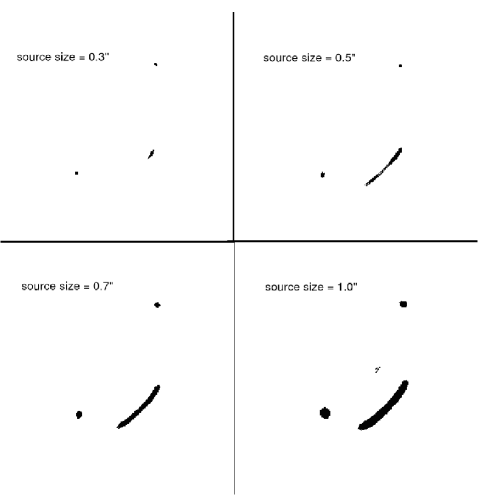
Figure 5.— Images of arcs produced by the same density map, at $z=0.3$, for sources, at $z=2$, of four different sizes.

Figure 6.— The averaged cross section over 30 density maps from a cluster at $z=0.3$ calculated using different source sizes.

Apart from the fact that cross section changes with changing source sizes, when we investigate the reason for the enhancement of lensing cross section due to the increase of source redshift (Wambsganss et al. Wambs (2004)), we realized that common assumptions made in the lensing simulations such as assuming a constant physical source size or constant angular source size will give different results that complicates cross comparisons between different simulations. We found that with constant physical source size and increasing source redshifts, lensing cross sections increases more dramatically than when we hold the angular source size constant. From this experiment, we can see that when we increase the source redshift, cross section increases not only due to the lensing weights, but also depends on the assumption made on the source sizes. This can be viewed as a manifestation of the effect of source sizes too, as we increase source redshifts, the sources (which we assumed to have constant physical sizes) appear to be smaller, thus contributing to the increase in cross section. We have shown the results in Table 2 that we run with 50 maps 10 different clusters.

$z$	cross section $(h^{-1}{\rm kpc})^{2}$
	constant angular size	constant physical size
1.00	0.203	0.203
1.25	1.220	1.627
1.50	4.882	9.153
2.00	15.662	33.358
3.00	33.968	77.597
4.00	46.579	86.445
5.00	54.308	121.633

Table 2Using 50 density maps taken from 10 different clusters, with a range of masses, varying source redshift, along with constant angular source size ($1^{\prime\prime}$) or physical source size ($11.2056h^{-1}$kpc which also translates to $1^{\prime\prime}$ at $z=1$).

While the cross section is somewhat sensitive to source size, we have found that other statistics, including those related to multiple arcs which are the main focus of this paper, are not very sensitive to the source size. For this reason we shall stick with a constant source size (of $1^{\prime\prime}$) and uniform intensity disks in our modeling. Calculations aimed at predicting the cross section should include a realistic source size distribution and redshift distribution.

Torri et al. Torri (2004) suggested that the strong lensing cross section has an interesting dependence on recent merger events. In particular, they have shown that merging clusters can have their cross sections enhanced by an order of magnitude during the merging process. This in principle could solve the discrepancy between the theoretical prediction and the observed number of giant arcs. However, they have used a cluster at $z\sim 0.3$ and artificially scaled its mass from $7\times 10^{14}\,h^{-1}M_{\odot}$ to $10^{15}\,h^{-1}M_{\odot}$ with the merging structure being 25% of the mass of the main cluster. It is not clear if such events are common enough to explain the RCS results. Further our studies suggest that truly efficient lenses arise when a large, contiguous region is above the critical density. Naively we imagine that mergers would lead to less “relaxed” high density material near the center of the cluster. This issue deserves further investigation, but we do not have the necessary simulations in hand at present.

As we have seen from the above discussion, the cross section of a cluster depends on many different, difficult to model, factors. This makes it challenging to predict the cross section and use these predictions as a probe of the background cosmology. Conversely it allows us to study many diverse phenomenon using a sample of giant arcs.

3. Central galaxies: ellipticities and orientations

One frequently finds massive galaxies at the center of clusters and this galaxy has a mass distribution which has been concentrated by the effects of baryonic cooling. This can affect the total mass profile in the region which is important for giant arc formation. Meneghetti et al. 2003b have argued that central galaxies have a substantial effect on cluster arc formation, while Dalal et al. Dalal (2004) have argued that they only affect arcs at small radii – though they isotropize the angular distribution of the arcs.

To investigate this, we artificially added central “galaxies” of different masses to the center of one of our simulated clusters. The galaxy was modeled as a randomly oriented ellipsoid with $q$ drawn uniformly in the range $[0.5,1]$. Figure 7 shows the increase in the giant arc cross section as a function of the mass of the added galaxy. At the higher mass end the giant arcs cross section is tripled. However we find, in agreement with Dalal et al. Dalal (2004), that the addition of central galaxies forms arcs primarily at small radii and there is an isotropization of the arc positions.

Figure 7.— The arc cross section as a function of the mass of the central galaxy added to 50 density maps, produced from projected densities of 50 different orientations of a cluster with mass $1.249\times 10^{1}5$ $h^{-1}M_{\odot}$. Note that when no galaxy is added, the result is indistinguishable from that of a galaxy of $5\times 10^{12}\,h^{-1}M_{\odot}$. The solid line is the cross section for arcs with $L/W>=7.5$, the dotted line is for arcs with $L/W>=10$.

Figure 8 shows that the lensing efficiency is much greater for some orientations of the central galaxy than others. In particular the efficiency is maximized when the central galaxy aligns with the projected mass of the underlying cluster, at $\phi\simeq 0.75$ in our example. Though the ellipticity of the central galaxy causes the cross section to fluctuate (see Fig. 9), the cross section does not seem to have a secular dependence on the (2D) ellipticities of the galaxies. This may be because several different factors are contributing to the effect. Depending on the ellipticities and the ratio of the size of the host cluster to the size of the central galaxy, the central galaxy will cover different fractions of area that are close to the super-critical region (region with super-critical surface density) of the cluster. This will modulate the cross section depending on the coverage of the cluster super-critical region.

Figure 8.— The dependence of the cross section on the orientation of the central galaxy. For each orientation there are 20 different ellipticities. We plot the average of 20 runs of galaxies lying in the same direction but with different ellipticities.

Figure 9.— The ellipticity of the central galaxies causes the cross section of the cluster to fluctuate. For each ellipticity there are 20 runs of different orientations of the galaxy. We plot the average of 20 galaxies with same ellipticities but different orientations.

In addition, we have observed that the more massive is the cluster to which the galaxy is added, the more dramatic the effect. Throughout our experiments we have found that the ability of a cluster to form giant arcs depends upon the number of pixels above critical in a contiguous region near the center. Adding a central galaxy to a high mass cluster brings the density from marginally critical to above critical over a wide region, thus increasing the formation of arcs for the more massive clusters. One might imagine that adding a galaxy to a low mass cluster would have a large effect, bringing a region from sub- to super-critical. However, since the cluster is low in mass it is difficult to bring a large contiguous region above the critical density, inhibiting efficient arc formation.

4. Giant arcs

4.1. The appearance of arcs

The arc distribution averaged over all the $32$ clusters, each with $32$ projections, appears to be primarily elliptical centered on the center of the clusters. The elliptical shapes resemble the critical curves of the elliptical clusters, and the centers of the arcs trace out the critical curves of the mass distribution. The width of the arcs depends on the source size, with sources smaller than $1^{\prime\prime}$ giving arcs which appear more similar to those seen in optical images.

As one realizes from simulations that most clusters are elliptical, and that their critical regions (regions enclosed by their critical curves) can be nicely fit by ellipses. We will discuss the appearance of arcs using terminologies that apply to ellipses to describe the lens. Please refer to upper figure in Fig.10 for the following discussion. Our arcs tend to form around points A, B , C and D of the elliptical critical region of the lens as this is also seen by Dalal et al. Dalal (2004).

The clusters with a more circular critical region tend to have more isotropically distributed arcs, while those with narrower critical regions give rise to arcs that reside mainly around points A and B of the critical regions.

Since clusters are mostly not perfect ellipse, there are clusters with distorted elliptical critical regions. When there is a curvature difference between point A and B (such as the lower figure in Fig.10), arcs are more likely to be found around point A (B) if the curvature around point A (B) is smaller than around point B (A).

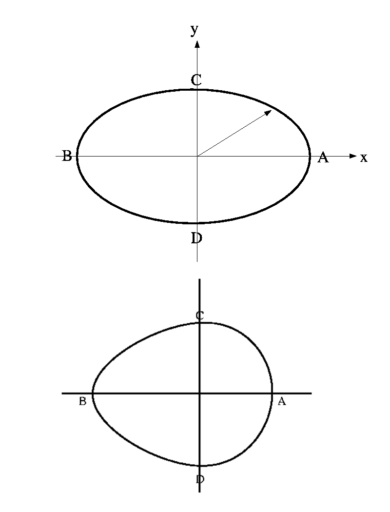
Figure 10.— The ellipses used for describing the critical region of the lens. The figure above describes the critical region as a ellipse, the figure below describes the critical region as a distorted egg-shaped ellipse.

This can be understood using a simple argument that there is a larger strip of critical curves that is available for arcs to reside and still be distinguished as unique arcs on the side with less curvature than the side with larger curvature.

4.2. Multiple arc systems

Multiple arcs are highly beneficial to determining the structure of clusters, and there appears to be more multiple arc systems than one would naively expect (e.g. Gladders et al. Gladders (2003)): for example, the RCS survey recently found that 2 out of their 5 arc forming clusters showed multiple arcs. Therefore, it is interesting to understand the prevalence of multiple arcs system and to add to our understanding of how the structure of clusters determine the formation of one or more arcs.

Using our pure dark matter maps and considering only 2 lens redshifts and 1 source redshift, we found 17 multiple arcs system out of 31 systems (with sources at $z=1$ and the lens at $z=0.3$ and $z=0.5$) that show arcs of L/W $>=7.5$. If we consider only the lensing systems that show the giant arcs (L/W $>=10$), we have 4 multiple giant arcs systems out of 9 giant arcs systems.

With a central galaxy, of mass $10^{13}\,h^{-1}M_{\odot}$, added to the center of the projected density maps and with sources at $z=1.0$ , we increase the number of arcs, but the fraction of multiple arc systems remains roughly unchanged (40-50%). When the lensing efficiency of the clusters increases (with increasing source redshifts), the fraction of multiple arc systems systematically increases. (see Table 3 for more statistics).

Maps Description	$L/W_{min}$	$z_{src}$	Multiple Arc
			Fraction
DM	10	1	4/9
DM	7.5	1	17/31
DM+cD	10	1	12/30
DM+cD	7.5	1	38/96
DM+cD	7.5	2	49/70
DM+cD	7.5	3	109/140
DM+cD	7.5	4	121/156

Table 3The multiple arc fraction (the ratio of number of multiple lensing systems to number of lensing systems) for different density maps. The first two row describes the result from dark matter only maps at $z=0.3$ and $z=0.5$. The remaining rows uses dark matter maps with an addition of a cD galaxy with maps at $z=0.3$. We also realize that with increasing lensing efficiency (at higher source redshifts), the ratio of number of multiple lensing systems increases.

Conversely, cutting out all arcs within $10^{\prime\prime}$ of the cluster center decreases the number of arcs but does not decrease the fraction of the multiple arc forming systems.

Finally, for a subset of the most massive clusters we verified that source size didn’t change the multiple arc fraction significantly. For sources from $0.2^{\prime\prime}$ to $1^{\prime\prime}$ the fraction decreased by only 8%. Also, the dependence of our multiple arc criterion on arc width is known to be weak. We infer from this that the fraction of multiple arc systems is relatively insensitive to the details of our modeling and can be calculated reasonably robustly using simulations such as ours.

Within the limited statistics, the fraction of multiple arc systems in our simulations agrees with the RCS observations. The arc geometries are also not too dissimilar, although the statistics in both our simulations and the observations are too poor to allow any strong statements to be made in this regard. The arc thickness depends on the source size and we would likely need to reduce our sources below $1^{\prime\prime}$ to get good visual agreement, but other properties are less sensitive to our modeling. We infer that the high percentage of multiple arc systems seen in RCS is not unexpected in a $\Lambda$CDM cosmology. The good agreement may be fortuitous, or it may be because both RCS and our simulations focused on massive clusters.

To understand the prevalence of multiple arcs we compute the arc multiplicity function. This lists the number of maps which have $N$ unique arcs. To compute this we threw many sources for each map and kept track of how many unique arcs were produced from those sources. Unfortunately we could find no unambiguous definition of “unique arcs”. Slight shifts in source position lead to arcs whose properties change continuously, making any clean separation difficult. To make progress we plotted the separations of different arcs and noted a drop in the number of arcs with distance at $3.4^{\prime\prime}$, at $z=0.3$. We picked this distance as a cut on whether an arc produced was just a repetition of the arcs that were produced before, or was a new arc. Our criterion for “unique arcs” was that the centers be separated by more than $3.4^{\prime\prime}$ at $z=0.3$. With this definition, the statistics of unique arcs seemed relatively insensitive to arc properties, such as width, and unique arcs usually came from distinct sources in the source plane, as seen in observations.

The multiplicity function is shown in Figure 11. Note that the vast majority of maps show no giant arcs. Among systems which show at least one arc however, a significant subset show multiple arcs. Note the extreme tails to this distribution, with maps that could in principle host tens of giant arcs were the sources properly aligned. This suggests that clusters in a $\Lambda$CDM cosmology could provide a rich array of arc possibilities, even before we consider substructure in the galaxies being lensed. While the probability that a cluster will host an arc, $p$, could be very small, once a lens is massive enough to host one arc the probability that it hosts a second is not suppressed by another power of $p$ (c.f. Gladders et al. Gladders (2003)).

Figure 11.— The arc multiplicity function: the number of maps which showed $N$ unique arcs of L/W $>=7.5$ (see text) when a large number of sources were thrown. The dotted line indicates the multiplicity function for clusters at $z=0.7$ with sources at $z=4.0$, the solid line shows the multiplicity function for clusters at $z=0.3$ with sources at $z=1.0$.

Among the $32$ clusters at $z=0.3$, we also find one “super-lensing” cluster. Three of the projections of this cluster, of the $4096$ total maps, produced $\sim 90\%$ of the arcs produced when we placed the sources at $z=1.0$. To understand this behavior we looked at the properties of the cluster in some detail. It is very massive, $M_{200}\simeq 1.5\times 10^{15}\,h^{-1}M_{\odot}$, and has its nearby structure residing almost in a plane (see Figure 12). When the line of sight is parallel to this plane not only the cluster but its neighbors and connecting filaments contribute to the projected mass “at” the lens, leading to a very efficient lensing configuration. The other orientations are not as efficient.

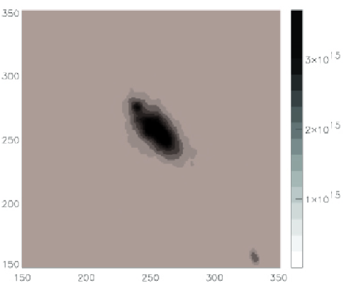
Figure 12.— (Upper) The projected mass (in $h^{-1}M_{\odot}/(h^{-1}{\rm Mpc})^{2}$) of the super-lensing cluster viewed in the plane where the nearby structure resides. The $x$- and $y$-axes are in pixels of size $9.77\,h^{-1}$kpc. (Lower) One example of a multiple arc system formed by this cluster.

It is interesting that the arc pattern of this super-lensing cluster is similar to the system RBS653 analyzed by Kausch et al. Kausch (2004), with multiple giant arcs formed at the two ends of the cluster. We do not have a large sample of such very massive, efficient clusters due to the limited volume we have simulated. It is not unreasonable to expect that observations, probing larger volumes, are picking up massive clusters which are highly efficient lenses, being surrounded by a large amount of correlated structure.

4.3. Mass distributions that are efficient in lensing

The existence of the super-lensing cluster leads us to ask: when would a mass distribution be a good lens? To answer this question we have taken our sample of simulated clusters and looked at the projected mass density of $\sim 20$ of them. They are all of similar mass and some are efficient lenses while the rest are not.

We noticed that the efficient clusters had reasonably large contiguous regions above $\Sigma_{\rm crit}$, while the less efficient clusters had separated regions above $\Sigma_{\rm crit}$. A reasonably sized contiguous region above $\Sigma_{\rm crit}$ typically has more sources which can be lensed sufficiently to form a giant arc. Looking at this from another viewpoint, we can also say that a larger contiguous super-critical region would mean the caustic extends over a larger region, thus giving rise to more lensing events in which sources (probably farther from each other) are forming arcs that are more likely to be apart in the image plane, thus easier to be uniquely identified. On the other hand, two separated regions (imagine we cut the previous contiguous region into two) above $\Sigma_{\rm crit}$ will then give rise to lensing events that consist of several sources very close to each other being lensed and form images that are fairly close to each other, thus harder to be distinguished as separate arcs, lowering the number of the arcs formed. This illustrates the fact that arcs merge complicates the correlation between the length of the caustic and the number of arcs that can be produced.

This observation also explains why the arc statistics are so sensitive to source redshift but less sensitive to central galaxies (apart from contribution from the change of source size due to changing source redshift). Imagine the cluster has a rather smooth mass distribution. Increasing $z_{\rm src}$ decreases $\Sigma_{\rm crit}$ and enlarges the region above critical density, giving rise to many more arcs. By contrast adding a central galaxy only brings the region near the center above critical, which may not be contiguous with other super-critical regions in the map.

5. Discussion and Conclusion

Recent observations have begun to amass statistics on giant arcs around clusters of galaxies. Such arcs probe the mass distribution of clusters on scales which should be amenable to theoretical interpretation (see Appendices), making lensing arcs a new meeting ground between theory and observation. This motivated us to consider how giant arcs are formed, and how one should use arcs to probe underlying clusters. To further our understanding in how arcs are formed, and how arcs can be used as a mass probe, we used ray tracing through N-body simulations to make simulated images of giant arcs. In addition to the dark matter followed by the simulations we have added analytic profiles representing central galaxies of various masses, orientations and ellipticities, used different source redshifts, source sizes and clusters at different redshifts to investigate the giant arcs statistics.

Our work is not the first to try understanding how arcs are formed. Where there is overlap our work agrees with some of the earlier simulations. In particular we agree with Dalal et al. Dalal (2004) on the effects of central galaxies and orientation of the cluster on the arc formation. We also agree with Wambsganss et al. Wambs (2004) on the strong dependence of arc cross section on source redshift, though we do not have enough information from their paper to make a precise comparison. We further the investigation of the strong redshift dependence, realized that with increasing source redshift, the cross section increases more drastically with constant physical source size than with constant angular source size. This redshift dependence may explain why RCS finds giant arcs in predominantly high-$z$ clusters. We agree with recent work suggesting that the link between the number of giant arcs and cosmology is complex, with assumptions about central galaxies, source redshifts, sizes, ellipticities and substructures making large differences in the theoretical predictions. We find in particular, and contrary to the claim by Bartelmann et al. Bart1 (1998), that the lensing cross section does depend on the source size assumed. This comes about through the selection of arcs above some fixed $L/W$ ratio, since the smaller the source size the narrower arc that is produced.

We investigated why some clusters are more effective lens than the others. We found a correlation between the area of the contiguous region above $\Sigma_{\rm crit}$ and the arc cross section. This helps to explain why certain clusters are better arc producers than other, comparable mass, clusters and why adding central galaxies is not as efficient as increasing the source redshift.

We have found one cluster in our simulations that is an extremely efficient lens. Given our relatively small simulation volume this suggests that CDM cosmologies should naturally produce clusters which are efficient arc, or even multiple arc, producers. Given the prevalence of multiple arcs systems in various observations, we investigated the multiple arcs system by looking at the number of unique arcs that arise from ray tracing our cluster sample. The fraction of systems producing multiple arcs in our simulations was quite insensitive to the details of our modeling, and close to the fraction seen in observations (Gladders et al. Gladders (2003)).

Looking forward into the future, upcoming wide-field observations such as RCSii, the CFHT Legacy Survey, the Sloan Digital Sky Survey and X-ray cluster surveys such as MACS can be expected to improve the statistics of giant arcs on the sky. With this increase in statistics we expect giant arcs will be an indispensable probe of the structure of clusters and the formation of large-scale structure.

Appendix A Comparison with analytic profiles

There is a large literature surrounding the theory of strong gravitational lensing, much of it based on simple analytic potentials (e.g. Narayan & Bartelmann Nara (1996), Keeton Keeton (2001), Kochanek et al. Kochanek (2004) and references therein). In order to understand how well such potentials describe our simulated clusters we compare here the critical curves and caustics of a select few of our clusters with those of the analytic form

$$\Sigma={\Sigma_{0}\over r(1+r^{2})}$$ (A1)

where $r=\left(qx^{2}+[y]^{2}/q\right)^{1/2}/R_{c}$. This analytic surface density is of a broken power-law form with finite mass, here taken to be $10^{15}\,h^{-1}M_{\odot}$. We set the scale radius to $R_{c}=70\,h^{-1}$kpc and the ellipticity ($q$) to $0.7$.

Arcs should be formed when the sources cross the caustics on the source plane where formally the magnification becomes infinite. The arcs trace out the critical curves in the image plane, being highly elongated and magnified images of the critical source.

We show the magnification of this analytic potential as a function of position in the source plane in Fig 12. Note the two ‘lips’ shaped structure commonly seen in potentials of this form. We can compare this to the same plot for two clusters from our N-body simulation (Fig 13). The first cluster is the “super-lensing” cluster (Fig. 12) of §4. Note the “squeezed diamond” shape of the magnification distribution for this cluster, which we are seeing projected edge-on. A less extreme example is given in the other panel of Fig 13.

We have found that the longer the caustic, the larger the cross section for lensing. This can be understood from the fact that there is a higher probability of the sources being largely magnified when we have a longer caustic. This is dramatically illustrated here: the cluster with shorter and smaller caustic (second panel) does not lens nearly as well as the cluster with the longer and larger caustic (first panel).

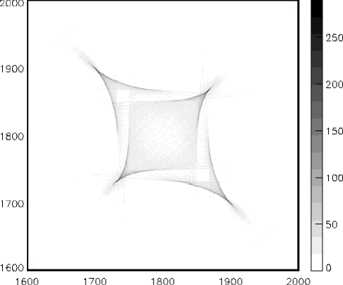
Figure 13.— A greyscale image of the magnification of the analytic potential as a function of position on the source plane (in pixels). Note the two lips shaped caustic structure.

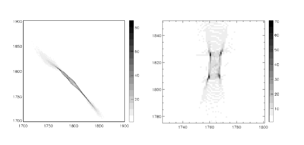
Figure 14.— Greyscale images of the magnification, as a function of position in the source plane (in pixels), of the super-lensing cluster described previously (left panel) and a cluster not being viewed edge-on (right panel). Again the caustic structure is clearly visible.

Appendix B Einstein Radius

The relevant scale for gravitational lensing is the Einstein radius, the radius of the circle formed by a spherically symmetric mass distribution lensing a perfectly on-axis source. It is useful to work through the calculation of the Einstein radius for the case of interest here. Solving the lens equation for an on-axis source being lensed by a spherically symmetric mass distribution we find

$$r_{E}=4\Delta\frac{GM(<r_{E})}{c^{2}r_{E}}$$ (B1)

where $M(<r)$ is the mass enclosed within radius $r$, $\Delta=D_{LS}D_{L}/D_{S}$ and $D_{L}$, $D_{LS}$ and $D_{S}$ are the angular diameter distances between the observer and the lens, the lens and the source, and the observer and the source respectively. If we define the (proper) gravitational radius of the lens as

$$r_{g}={4GM_{\rm tot}\over c^{2}}$$ (B2)

we can rewrite Eq. B1 as

$$\left({r_{E}\over R_{*}}\right)^{2}={M(<r_{E})\over M_{\rm tot}}$$ (B3)

where $R_{*}\equiv\sqrt{r_{g}\Delta}$. For a $10^{15}\,h^{-1}M_{\odot}$ lens at $z\simeq 0.3$ and sources at $z\simeq 1$ the characteristic scale $R_{*}\simeq 300\,h^{-1}$kpc comoving. The scale is relatively insensitive to the source and lens redshift, within the interesting range $R_{*}$ lies between $300$ and $450\,h^{-1}$kpc. Typically $r_{E}<R_{*}$.

To solve Eq. B3 we need to assume a profile $M(<r)$. Unfortunately for an NFW profile the solution is quite unstable, because $M(<r)\sim r^{2}$ for $r\to 0$. Small changes in the assumed mass or lensing geometry can dramatically alter the solution for $r_{E}$. This is one of the reason why the ability of clusters to form arc has such a strong dependence on e.g. the viewing orientation. Physically this extreme sensitivity is mitigated by the presence of a central cusp in the mass distribution which is steeper than $\rho\sim r^{-1}$ for $r\to 0$, for example a central galaxy with an isothermal profile. Thus for many systems the defining scale is set by the radius at which baryonic cooling has steepened the central profile beyond $1/r$. The Einstein radius is then determined by the galactic radius and is of order $100$kpc.

References

- (1) Bartelmann, M., Huss, A., Colberg, J. M., Jenkins, A., & Pearce, R. R. 1998, A&A, 330, 1
- (2) Bartelmann, A., Meneghetti, A., Perrotta, F., Baccigalupi, C., & Moscardini, L. 2003, A&A, 287, 1
- (3) Blain, A. W., Kneib, J.-P., Ivison, R. J., & Smail, I. 1999, ApJ, 512, L87
- (4) Dalal, N., Holder, G. & Hennawi, J. F. 2004, ApJ, 609, 50
- (5) Davis, M., Efstathiou, G., Frenk, C. S., White, S. D. M. 1985, ApJ, 292, 371
- (6) Gladders, M. D., Hoekstra, H., Yee, H. K. C., Hall, P. B. & Barrientos, L. F. 2003, ApJ, 593, 48
- (7) Hockney, R. W., Eastwood, J. W. 1980, “Computer Simulation Using Particles”, New York, McGraw-Hill
- (8) Kausch, W., Schindler, S., Kronberger, T., Wambsganss, J., Schwope,A., Erben, T. 2004, preprint (astro-ph/0406107)
- (9) Keeton, C. 2001, preprint (astro-ph/0102341)
- (10) Kochanek, C.S., Schneider, P., Wambsganss, J., Part 2 of Gravitational Lensing: Strong, Weak & Micro, Proceedings of the 33rd Saas-Fee Advanced Course, G. Meylan, P. Jetzer & P. North, eds. (Springer-Verlag: Berlin)
- (11) Luppino, B. A., Gioia, I. M., Hammer, F. , Le Fevre, O., & Annis, J. A. 1999, A&AS, 136, 117
- (12) Macciò, A. V. 2004, preprint (astro-ph/0402657)
- (13) Meneghetti, M., Bartelmann, M., & Moscardini, L. 2003, MNRAS, 346, 67
- (14) Meneghetti, M., Bartelmann, M., & Moscardini, L. 2003, MNRAS, 340, 105
- (15) Meneghetti, M., Bartelmann, M., Dolag, K., Moscardini, L., Perrotta, F., Baccigalupi, C., Tormen, G. 2004, preprint (astro-ph/0405070)
- (16) Metcalfe, L., Kneib, J.-P., McBreen, B., Altieri, B., Biviano, A., Delaney, M., Elbaz, D., Kessler, M. F., Leech, K., Okumura, K., Ott, S., Perez-Martinez, R., Sanchez-Fernandez, C., & Schulz, B. 2003, A&A, 407, 791
- (17) Narayan, R., Bartelmann, M. 1996, preprint (astro-ph/9606001)
- (18) Navarro, J. F., Frenk, C. S. & White, S.D. M. 1997, ApJ, 490, 493
- (19) Oguri, M., Lee, J., & Suto, Y. 2003, ApJ, 599, 7-23
- (20) Perlmutter, S. et al. 1999, ApJ, 517, 565
- (21) Riess, A.B. et al. 1998, Phys. Rev. D, 37, 3406
- (22) Sand, D., Treu, T., Smith, G. P., Ellis, R. S. 2004, ApJ, 604, 88
- (23) Schwope, A., Hasinger, G., Lehmann, I., Schwarz, R., Brunner, H., Neizvestny, S., Ugryumov, A., Balega, Yu., Trumper, J., Voges, W. 2000, AN, 321, 1
- (24) Smail, I., Ivison, R. J., Blain, A. W., & Kneib, J.-P. 2002, MNRAS, 331, 495
- (25) Spergel, D. N., Verde, L., Peiris, H. V., Komatsu, E., Nolta, M. R., Bennett, C. L., Halpern, M., Hinshaw, G., Jarosik, N., Kogut, A., Limon, M., Meyer, S. S., Page, L., Tucker, G.S., Weiland, J. L., Wollack, E., & Wright, E. L. 2003, Astrophys. J. Supp., 148, 175
- (26) Tegmark, M., Zaldarriga, M., & Hamilton, A., J. 2001, Phys. Rev. D, 63, 43007
- (27) Torri, E., Meneghetti, M., Bartelmann, M., Moscardini, L.,Rasia, E., Tormen, G. 2004, MNRAS, 349, 476
- (28) Wambsganss, J., Bode, P., & Ostriker, J. P. 2004, ApJ, 606, L93
- (29) White, M. 2002, Astrophys. J. Supp., 143, 241
- (30) William, L. L. R., Navarro, J. F., & Bartelmann, M. 1999, ApJ, 527, 535
- (31) Yan, R., White, M., Coil, A. L. 2003, ApJ, 598, 848
- (32) Zaritsky, D. & Gonzales, A. H. 2003, ApJ, 584, 691