Investigating the origins of the CMB-XRB cross correlation

Abstract

Recently, we presented evidence for a cross-correlation of the $WMAP$ satellite map of the cosmic microwave background (CMB) and the $HEAO1$ satellite map of the hard X-ray background (XRB) with a dimensionless amplitude of $0.14\pm 0.05$ normalized to the product of the $rms$ fluctuations of the $CMB$ and $XRB$ (Boughn & Crittenden, 2004). Such a correlation is expected in a universe dominated by a cosmological constant via the integrated Sachs-Wolfe (ISW) effect and the level of the correlation observed is consistent with that predicted by the currently favored Lambda cold dark matter ($\Lambda CDM$) model of the universe. Since this offers independent confirmation of the cosmological model, it is important to verify the origin of the correlation. Here we explore in detail some possible foreground sources of the correlation. The present evidence all supports an ISW origin.

1 Introduction

In a remarkably short time, the standard cosmological model has changed from a Friedmann universe to a spatially flat universe that is dominated by a cosmological constant or some other form of dark energy (e.g., Bahcall et al. 1999). So far, the primary evidence for this model comes from supernovae redshift/magnitude observations (Riess et al. 2004) that imply the expansion of the universe is accelerating and from the spatial power spectrum of the fluctuations in the cosmic microwave background (Bennett et al., 2003). While these pieces of evidence are compelling, especially when combined with the clustering and density of matter deduced from galaxy observations, it is clearly desirable to to seek independent confirmation of the $\Lambda CDM$ model.

The late-time integrated Sachs-Wolfe (ISW) effect (Sachs & Wolfe 1967) promises to provide such an independent test. In a $\Lambda$ dominated universe CMB photons undergo a net energy shift when traversing linear density perturbations (i.e., $\delta\rho/\rho<<1$) at relatively low redshifts ($z\mathrel{\raise 1.50696pt\hbox{$\scriptstyle<$}\kern-6.00006pt\lower 1.72218pt\hbox{{$\scriptstyle\sim$}}}1$). Crittenden and Turok (1996) suggested that the ISW effect could be detected by correlating the CMB with some nearby ($z\mathrel{\raise 1.50696pt\hbox{$\scriptstyle<$}\kern-6.00006pt\lower 1.72218pt\hbox{{$\scriptstyle\sim$}}}1$) tracer of matter, e.g., galaxies or AGN. This also occurs in a matter dominated universe with less than the critical density; however, the effect is spread over larger redshifts (Kamionkowski 1996). Initial attempts to detect such an ISW signal (Boughn, Crittenden, & Turok 1998; Kamionkowski & Kinkhabwala 1999; Boughn & Crittenden 2002; Boughn, Crittenden & Koehrsen 2002) led only to upper limits on $\Lambda$ in a flat $\Lambda CDM$ universe and on the curvature density in an open, matter dominated universe.

The situation changed recently with the release of the first year of data from the $WMAP$ satellite (Bennett et al. 2003). Since then, six teams have found correlations of the $WMAP$ CMB data with tracers of matter including the hard ($2-10~{}keV$) X-ray background, the NVSS radio galaxy survey, the APM galaxy survey, the Sloan Digital Sky Survey, and the 2MASS infrared galaxy survey (Boughn& Crittenden 2004a; Nolta, et al. 2004; Myers et al. 2004; Fosalba & Gaztanaga 2004; Scranton et al. 2003; Afshordi, Loh, & Strauss 2004). All of these results are only marginally statistically significant, $\mathrel{\raise 1.50696pt\hbox{$\scriptstyle<$}\kern-6.00006pt\lower 1.72218pt\hbox{{$\scriptstyle\sim$}}}3~{}\sigma$; however, most of them detect an ISW signal with an amplitude similar to that predicted by the $\Lambda CDM$ model. The X-ray/CMB cross-correlation (Boughn & Crittenden 2004) is, perhaps, the most statistically significant detection, thanks to the large area covered by the X-ray data and the fact the the AGN sources are at somewhat higher redshifts. It is the purpose of the present paper to provide the details of the X-ray/CMB correlation analysis and to demonstrate that this correlation is unlikely to be due to contamination by foregrounds, such as microwave emission from X-ray sources or from Galactic emission.

2 The $HEAO1~{}A2~{}2-10~{}keV$ X-ray Map

The HEAO1 data set we consider was constructed from the output of two medium energy detectors (MED) with different fields of view ($3^{\circ}\times 3^{\circ}$ and $3^{\circ}\times 1.5^{\circ}$) and two high energy detectors (HED3) with these same fields of view (Boldt 1987). The data were collected during the six month period beginning on day 322 of 1977. Counts from the four detectors were combined and binned in 24,576 $1.3^{\circ}\times 1.3^{\circ}$ pixels. The pixelization we use is an equatorial quadrilateralized spherical cube projection on the sky (White and Stemwedel 1992). The combined map has a spectral bandpass (quantum efficiency $\mathrel{\raise 1.50696pt\hbox{$\scriptstyle>$}\kern-6.00006pt\lower 1.72218pt\hbox{{$\scriptstyle\sim$}}}50\%$) of approximately $3-17~{}keV$ (Jahoda & Mushotzky 1989). For consistency with other work, all signals are converted to equivalent flux in the $2-10~{}keV$ band.

Because of the ecliptic longitude scan pattern of the HEAO satellite, sky coverage and, therefore, photon shot noise are not uniform. However, the variance of the cleaned, corrected map, $2.1\times 10^{-2}~{}(TOT~{}counts~{}s^{-1})^{2}$, is significantly larger than the mean variance of photon shot noise, $0.8\times 10^{-2}~{}(TOT~{}counts~{}s^{-1})^{2}$, where $1~{}TOT~{}counts~{}s^{-1}\approx 2.1\times 10^{-11}erg~{}s^{-1}cm^{-2}$ (Allen, Jahoda & Whitlock 1994). This implies that most of the variance in the X-ray map is due to “real” structure. For this reason and to reduce contamination from any systematics that might be correlated with the scan pattern, we chose to weight the pixels equally in this analysis. However, weighting the pixels in proportional to their sky coverage makes little difference in the subsequent analysis.

The resulting map of the hard X-ray background (XRB) has several foreground features that were fit and removed from the map: a linear time drift of detector sensitivity, high latitude Galactic emission, the dipole induced by the earth’s motion with respect to the XRB, and emission from the plane of the local supercluster. These corrections are discussed in detail in Boughn (1999) and in Boughn, Crittenden, & Koehrsen (2002). The map was also aggressively masked by removing all pixels within $20^{\circ}$ of the Galactic plane and within $30^{\circ}$ of the Galactic center. In addition, large regions ($6.5^{\circ}\times 6.5^{\circ}$) centered on $92$ nearby, discrete X-ray sources with $2-10~{}keV$ fluxes larger than $3\times 10^{-11}erg~{}s^{-1}cm^{-2}$ (Piccinotti et al. 1982) were removed from the maps. Around the sixteen brightest of these sources (with fluxes larger than $1\times 10^{-10}erg~{}s^{-1}cm^{-2}$) the masked regions were enlarged to $9^{\circ}\times 9^{\circ}$.

Finally, the map itself was searched for “sources” that exceeded the nearby background by a specified amount. Since the ‘quad-cubed’ pixelization format lays out the pixels on an approximately square array, we averaged each pixel with its eight neighbors and then compared this value with the median value of the next nearest sixteen pixels (ignoring pixels within the masked regions). If the average flux associated with a given pixel exceeded the median flux of the background by a prescribed threshold (1.75 times the mean shot noise), then all 25 pixels ($6.5^{\circ}\times 6.5^{\circ}$) were removed from further consideration. The result of all these cuts is a map with $33\%$ sky coverage. This was the same map that was used in previous attempts to detect a correlation of the the XRB and CMB (Boughn, Crittenden, & Turok 1998; Boughn, Crittenden, & Koehrsen 2002) and is used as our canonical X-ray map in the following analysis. We have also used other maps with less aggressive source removal and the correlation results are nearly independent of these cuts; although, the less aggressively masked maps result in somewhat higher noise. For details of the various source cutting schemes, see Boughn, Crittenden, & Koehrsen (2002).

3 The $WMAP$ CMB Map

The primary CMB map used in the following analysis is the “internal linear combination” (ILC) map derived from the first year of data from the $WMAP$ satellite (Bennett et al. 2003) re-pixelized to be in the same format as the HEAO X-ray map. The ILC map was constructed so as to have little contamination from the Galaxy; however, to avoid any residual low Galactic latitude contamination, we masked it with the most aggressive $WMAP$ Galaxy mask ($k0$) from Bennett et al. (2003), which results in $68\%$ sky coverage. For the $1.3^{\circ}$ angular resolution of the ILC map, instrument noise is negligible so we chose to weight each of the unmasked pixels equally in all subsequent analyses. To check our results we also used the independently derived “cleaned” map of Tegmark, de Oliveira-Costa, and Hamilton (2003). It is not surprising that this map yielded results that were consistent with the ILC map since the two maps were derived from the same primary data. To check for a possible frequency dependence of the results we also used Q-band (41 GHz), V-band (61 GHz), and W-band (94 GHz) $WMAP$ maps with the same $k0$ masking. The correlation results of these three maps are also indistinguishable from the ILC map as will be discussed below.

4 The CMB/XRB Cross-correlation Function

A standard measure of the correlation of two data sets is the cross-correlation function ($CCF$), which in this case is defined by

$$CCF(\theta)={1\over N_{\theta}}\sum_{i,j}(I_{i}-\bar{I})(T_{j}-\bar{T})$$ (1)

where the sum is over all pairs of pixels $i,j$ separated by an angle $\theta$, $I_{i}$ is the X-ray intensity of the $i$th pixel, $\bar{I}$ is the mean intensity, $T_{i}$ is the CMB temperature of the $i$th pixel, $\bar{T}$ is the mean CMB temperature, and $N_{\theta}$ is the number of pairs of pixels separated by $\theta$. The $CCF(\theta)$ generated from the “cleaned” map is consistent with but typically $\sim 10\%$ larger than that generated from the ILC map. The average of these two $CCF$s is shown in Figure 1. The $CCF$ in this figure appears to reveal a considerable level of cross-correlation on angular scales $\theta\mathrel{\raise 1.50696pt\hbox{$\scriptstyle<$}\kern-6.00006pt\lower 1.72218pt\hbox{{$\scriptstyle\sim$}}}10^{\circ}$. However, this is a bit misleading since the error bars in Figure 1 are highly correlated.

We estimated the standard deviations and correlation matrix of the errors in the $CCF$ in two ways. Using the data themselves, we computed 400 $CCF$s by rotating the ILC and “cleaned” maps with respect to the X-ray map. By performing two rotations of angles larger than $20^{\circ}$, the effects of any intrinsic correlations at small angular scales, $\theta\mathrel{\raise 1.50696pt\hbox{$\scriptstyle<$}\kern-6.00006pt\lower 1.72218pt\hbox{{$\scriptstyle\sim$}}}10^{\circ}$, are minimized. Of course, there were pixels pairs that are repeated in some rotations; however, the number of these are very small compared to the number of pixel pairs at each angle $\theta$. While the signal distribution in the maps is to a good approximation Gaussian, this method enabled us to estimate the errors in a way that is relatively independent of the statistical characteristics of the noise in the maps. As an alternative we generated 1000 Monte Carlo CMB maps expected from Gaussian fluctuations with the $\Lambda CDM$ cosmological parameters consistent with the $WMAP$ data set. These Monte Carlo maps were cross-correlated with the the real X-ray map. We did not generate Monte Carlo X-ray maps since the XRB is not as well characterized statistically as the CMB. That the standard deviations and noise correlation matrices of these two methods agree to within a few percent is an indication that the errors are well characterized to this level. Since we did not generate Monte Carlo X-ray maps, there was no correlated component in the Monte Carlo trial maps and, therefore, cosmic variance of the ISW signal was ignored. Because of the large sky coverage, the cosmic variance noise of the ISW effect is considerably smaller than other noise sources and, in any case, does not change the statistical significance of the detection of a correlated signal in the two maps.

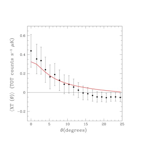
Figure 1: The points show the cross correlation observed between the WMAP and HEAO-A2 data sets. The heavy solid line represents the predictions for the best fit WMAP $\Lambda CDM$ cosmology.

The $CCF$ due to the ISW effect should be achromatic, i.e., independent of the frequency at which the CMB is observed (unlike the Sunyaev-Zel’dovich effect). To check this the X-ray map was cross-correlated with three $WMAP$ CMB maps at frequencies $41\pm 4~{}GHz$ (Q-map), $61\pm 7~{}GHz$ (V-map), and $94\pm 10GHz$ (W-map). These three maps were corrected for Galactic emission using the synchrotron, free-free, and dust maps from the WMAP public data set. The resulting CCFs are plotted in Figure 2. If the positive correlation reported here were due to radio source contamination, one would expect the Q-band CCF to be considerably larger than the the W-band CCF, which is clearly not the case. The case against radio source contamination is discussed in detail in §6.3 below.

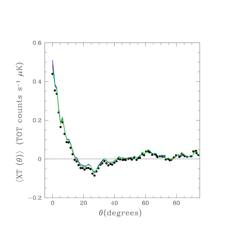
Figure 2: The cross correlations using the various WMAP frequencies ($Q,V$ and $W$) are all consistent with that found using the ILC map. The nearly coincident red, green and blue curves are CCFs of the X-ray map with the 41, 61, and 94 $GHz$ CMB maps while the points are from Figure 1. Much stronger frequency dependence would be expected were the signal arising with a typical spectral index expected for radio sources.

5 The significance of the detection

The first three points plotted in Figure 1 ($0^{\circ}\leqslant\theta\leqslant 2.8^{\circ}$) are more than $2~{}\sigma$ greater than zero while the next four points ($4.0^{\circ}\leqslant\theta\leqslant 7.8^{\circ}$) all exceed zero by more than $1~{}\sigma$. However, due to the highly correlated nature of the noise, the overall statistical significance of the detection is only $\sim 3~{}\sigma$ as will be discussed below.

Since each of the values of the $CCF$ is determined from a great many pixel pairs (from $7.2\times 10^{3}/$ pairs for the $\theta=0^{\circ}$ point to $1.5\times 10^{6}/$ for $\theta=90^{\circ}$), it is reasonable to assume that the noise in the $CCF$ is Gaussian distributed (by the central limit theorem). Indeed, the observed distributions of the both the 1000 Monte Carlo trials and the 400 rotated map trials were consistent with Gaussianity. As a test of the tails of the distribution we noted the number of times the $CCF(0)$ values of the noise trials exceeded that level observed in Figure 1. Out of the 1000 Monte Carlo trials, the noise exceeded this level 8 times, i.e., $0.008\%$ of the time. This corresponds to a $2.4~{}\sigma$ effect which is consistent with the value of $2.5~{}\sigma$ of Figure 1. Similar agreement was found for the rotated map trials and for other separation angles.

To determine the overall statistical significance of the detection of the ISW effect requires an ISW model. However, the likelihood that the observed $CCF$ is due to noise alone (with no intrinsic correlation of the two maps) can be evaluated in the absence of any model. $\chi^{2}$ provides such an estimate, i.e.,

$$\chi^{2}=\sum_{ij}CCF(\theta_{i})(C_{ij})^{-1}CCF(\theta_{j})$$ (2)

where $(C_{ij})^{-1}$ is the inverse of the noise correlation matrix. $\chi^{2}$ is a conservative estimate of significance since it only assumes Gaussian noise and nothing about the nature of the signal (other than our expectation that the signal occurs at small angles $\theta\mathrel{\raise 1.50696pt\hbox{$\scriptstyle<$}\kern-6.00006pt\lower 1.72218pt\hbox{{$\scriptstyle\sim$}}}10^{\circ}$). In any case, depending on the number of data points included in the sum, the null hypothesis is excluded at the $93\%$ to $99\%$ C.L., the latter of which is for the first 8 data points ($\theta\leqslant 9^{\circ}$) with $\chi_{\nu}^{2}=19.5/8$.

The ISW effect provides a prediction for the shape and amplitude of the correlation for a given $\Lambda$. Since the shape varies little as $\Lambda$ varies, we can use it as a template and fit for the amplitude. Doing this, the best fit amplitude of the dimensionless correlation function (normalized to the rms fluctuations of the CMB and XRB) at $\theta=0^{\circ}$ ranges from $0.118\pm 0.049$ ($2.40~{}\sigma$, 99.2 % C. L., $\chi^{2}=1.0/1$) for a fit to the first two data points to $0.141\pm 0.048$ ($2.94~{}\sigma$, $99.8$ C.L., $\chi^{2}=10.9/7$) for a fit to the first 8 data points. We take the latter as our canonical fit and note that the fit to the first 7 data points gives the same result. Fits using from 4 to 8 data points vary by only $\pm 6\%$.

In the above analysis we have assumed that the noise in both the X-ray and CMB maps is Gaussian and this is supported by the pixel distribution functions of the X-ray intensity and CMB temperature. As will be seen below, the distribution of the product of signals in pixel pairs is also well fit by that expected for Gaussian processes as shown in Figures 3 and 4a. Finally, the frequency with which the $CCF(\theta)$ generated by Monte Carlo trials exceed a given level are consistent with that expected from Gaussian processes out to $3~{}\sigma$. The fact that the trials generated from rotated versions of the maps agreed with the Monte Carlo trials also indicates that the noise is statistically well understood. So from a statistical point of view, our $3~{}\sigma$ results is well characterized by a $0.999\%$ confidence level.

In the present case, the dominant source of “noise” is the fluctuations in the CMB from the surface of last scattering and cannot be easily eliminated. Even if instrument noise were negligible and the Poisson noise associated with the discreteness of the X-ray sources could be eliminated, one would expect only a factor of 2 improvement in signal to noise (Crittenden & Turok 1996). It will be some time before the next generation of surveys (e.g., the Large Synoptic Survey Telescope and the Square Kilometer Array) provides us with new, large-scale mass tracers that will enable this improvement to be realized.

6 Possible Systematic Errors

Since the significance of the detection is limited, it is essential that we carefully consider possible systematics which could contribute to the cross correlation.

6.1 Localized contamination

One important issue is discovering if the signal we observe is due to strong correlations between a few contaminated pixels, or is due to relatively weak correlations on the whole sky, as predicted by the ISW effect. One test of this is to split the data into two hemispheres. The fits of the amplitude of the dimensionless correlation function to the north and south Galactic hemispheres are $0.17\pm 0.07$ ($\chi^{2}=5.3/7$) and $0.11\pm 0.07$ ($\chi^{2}=13.8/7$) using the first 8 data points. While the noise in the detection increases, the signals seen in both hemispheres are clearly consistent with each other.

Another test for localized contamination is to examine the distribution function of the individual terms contributing to the $CCF$ of Equation 1, i.e., $(I_{i}-\bar{I})(T_{j}-\bar{T})$. To a good approximation, the individual pixel distribution functions of both maps are Gaussian. If the correlated component of the two maps arises from the linear ISW effect, then the values of $(I_{i}-\bar{I})$ and $(T_{j}-\bar{T})$ should be consistent with a bivariate Gaussian distribution with dimensionless cross-correlation coefficient $c(\theta)=CCF(\theta)/(\sigma_{T}\sigma_{X})$, where $\sigma_{X}^{2}=\langle(I_{i}-\bar{I})^{2}\rangle$ is the variance of the X-ray intensity and $\sigma_{T}^{2}=\langle(T_{i}-\bar{T})^{2}\rangle$ is the variance of the CMB temperature. ($\sigma_{X}=0.124~{}TOT~{}cnts~{}s^{-}1$ and $\sigma_{T}=64\mu K$ for the maps we used.) It is straightforward to show (see Appendix A) that the distribution function, $dN/d\mu$, for the product $\mu=(I_{i}-\bar{I})(T_{j}-\bar{T})/\sigma_{T}\sigma_{X}$ is given by

$$dN/d\mu={N_{\theta}e^{c(\theta)\mu^{\prime}}K_{0}(\mu^{\prime})\over\pi(1-{c(\theta)}^{2})^{1/2}}$$ (3)

where $K_{0}$ is the modified Bessel function, $\mu^{\prime}=\mu/(1-{c(\theta)}^{2}),$ and $N_{\theta}$ is the number of pixel pairs separated by an angle $\theta$. Figure 3 is a typical plot of the distribution of pixel pairs (in this case for the $\theta=2.7^{\circ}$ bin), as a function of $\mu$ along with the theoretical curve given in Equation 3. The error bars are the usual Poisson error bars, i.e., $\sqrt{n}$ where $n$ is the number of pixel pairs in the relevant bin. The theoretical curve is not a fit to the distribution function data but rather uses the average value of $c(\theta)$ determined by Equation 1. The difference between the observed distribution $(dN/d\mu)_{obs}$ and the theoretical distribution of Equation 3 $(dN/d\mu)_{theo}$ for the data of Figure 3 is plotted in Figure 4a as fractional residuals, i.e., $((dN/d\mu)_{obs}-(dN/d\mu)_{theo})/(dN/d\mu)_{theo}$. For comparison, Figure 4b is a plot of the fractional residuals assuming $c(\theta)=0$, i.e., in the absence of correlations. The nearly straight line in Figure 4b is the theoretical curve with correlations and its slope is a measure of the positive cross-correlation, $c(\theta)$. It is clear from this plot that the cross-correlation is manifested for the full range of $\mu$. Were the correlation due to a limited number of non-Gaussian pixel pairs with large values of $\mu$, one would expect significant deviations from the linear behavior exhibited in Figure 4b.

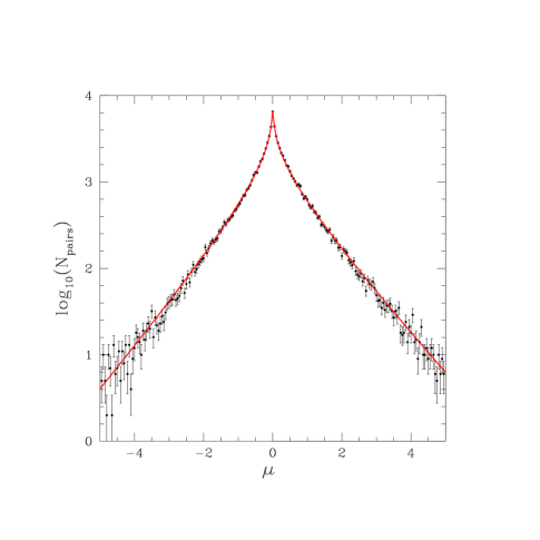
Figure 3: Each bin of the observed correlation in Figure 1 is the average of products of pairs of pixels of the X-ray and CMB maps. This shows the distribution of the products for all the pixel pairs contributing to the $2.7^{\circ}$ bin, normalized by the rms values of the two maps. This figure and the next demonstrate that the observed correlation is not arising from a few pixels pairs, but is coming from an asymmetry in the full distribution, precisely as expected from a weak correlation of two Gaussian fields.

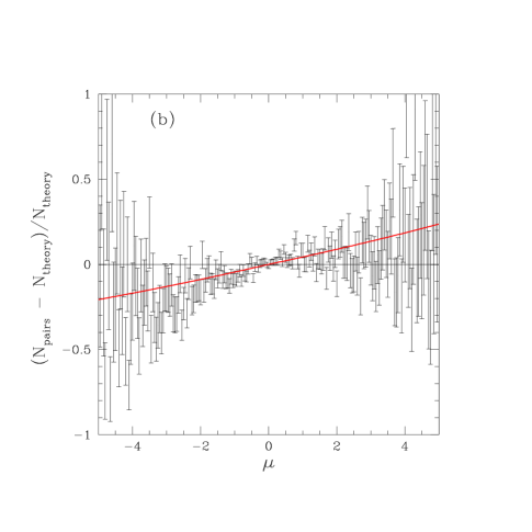
Figure 4: (a) The fractional differences between the observed distribution seen in Figure 3 and that predicted for the correlation given in Figure 1 at $\theta=2.7^{\circ}$. The Poisson error bars are largest at large $\mu$ where there are the fewest pixels pairs. (b) The fractional differences between the observations and the prediction for uncorrelated Gaussian fields. The heavy line corresponds to the correlated model used in (a) and the data are clearly consistent with the theoretical curve over the whole range of $\mu$’s.

Equation 1 determined the $CCF(\theta)$ from a straight average of the correlation arising from the pixel pairs. Alternatively, we can fit the distributions (such as Figure 3) for the best dimensionless correlation $c(\theta)$ for each angular bin. To do this, we consider a statistic $\sum_{i}((dN/d\mu)_{obs}(\mu_{i})-(dN/d\mu)_{theo}(\mu_{i}))^{2}/n_{i}$ where the sum is over the the bins at $\mu_{i}$ and $n_{i}$ is the number of pixel pairs in the $i^{th}$ bin, i.e., the Poisson variance. Minimizing this statistic with respect to $c(\theta)$ yields another unbiased estimate for the cross-correlation function $CCF(\theta)$. Figure 5 is the average correlation function of such fits to the ILC and “cleaned” CMB maps for a fit range of $-4.0<\mu<4.0$. The $CCF(\theta)$ determined in this way is consistent with the $CCF$ derived from Equation 1 and depicted in Figure 1. The errors in Figure 4 were determined from the same 1000 Monte Carlo trials discussed above. Importantly, these estimates were insensitive to the domains of the fits; i.e., fitting the function over the interval $-5.0<\mu<5.0$ was consistent with that for the interval $-1.0<\mu<1.0$. This is evident for the example given in Figure 4b where the slope provides a reasonable fit to the data over the entire range of $\mu$.

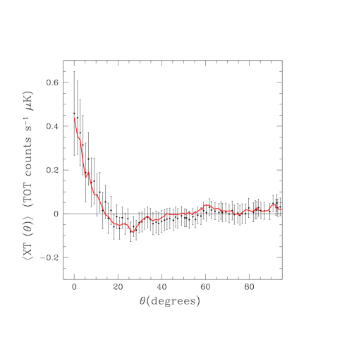
Figure 5: The cross-correlation function estimated by fitting Equation 3 to the distribution function of pixel pairs (e.g., Figure 3) for all angular separations. These fits were restricted to pixel pair amplitudes of $|\mu|\leqslant 4$. The results are consistent with the CCF of Figure 1 (solid line) and imply that the correlation is not arising from a few contaminated pixels.

6.2 Instrumental systematics

In general, cross-correlations are relatively insensitive to unknown systematic instrumental errors, especially if the two data sets are as disparate as the $HEAO$ X-ray map and the $WMAP$ CMB map considered here. It is difficult to imagine how systematic errors related to the instruments could be correlated with each other. To be sure, if the systematics are extremely large, then even a small correlation between them could generate a significant $CCF$. However, any residual systematics in the $WMAP$ data appear to be far below the level of inherent fluctuations in the CMB (Bennett et al. 2003). The $HEAO$ X-ray map does suffer from a significant linear drift in detector sensitivity (Jahoda 1993) but we have fit for and removed this effect down to a level below that of the intrinsic fluctuations of the XRB (Boughn 1998). Also, the instrument drift results in a signal proportional to ecliptic longitude and, therefore, represents a larger angular scale structure than that in Figure 1 . Thus we conclude it is quite unlikely that instrument related systematics are responsible for the observed correlations.

6.3 Foreground radio sources

More problematic might be the microwave emission of foreground radio sources that also emit in hard X-rays. Certainly radio sources are highly correlated with the X-ray background (Boughn 1998) and if these sources also emit significantly at microwave frequencies then a positive correlation between the CMB and the XRB would be expected. If this were the case, the $CCF$ would have the same profile as the X-ray auto-correlation function ($ACF$). However, the $CCF$ profile in Figure 1 is substantially broader than the X-ray $ACF$ with a half maximum width of $\sim 4^{\circ}$ for the former and $\sim 2^{\circ}$ for the latter (Boughn, Crittenden, & Koehrsen 2002). In addition, the analysis of the distribution function discussed above effectively eliminates the possibility that the $CCF$ signal is due to a few “ringers”, i.e., a few regions of the sky that are coincidentally bright (or dim) in both the X-ray and CMB.

We can attempt to directly estimate the microwave emission of the sources of the hard X-ray background. However, this is difficult since recent surveys have not been extensive and are limited to relatively low frequencies ($<5$ GHz); in addition, radio emission is only very roughly proportional to X-ray luminosity. Never-the-less, we have made rough estimates by transforming the low frequency radio data to WMAP frequencies assuming a power spectral index of $\alpha\sim-0.4$, which is the average observed for X-ray selected radio sources (e.g., Reich et al. 2000). Using the ROSAT/FIRST analysis of X-ray bright AGN by Brinkmann et al. (2000), we obtain a rough estimate of the ratio of the 41 GHz radio flux density to 2-10 keV X-ray flux for these sources, $\log(F_{\nu}/F_{X})=-14.2$. Combining this with the $rms$ fluctuation of the X-ray background, $1.5\times 10^{-9}~{}ergs~{}s^{-1}cm^{-2}sr^{-1}$ (Boughn, Crittenden, Koehrsen 2002), the implied correlated component of the 41 GHz CMB temperature fluctuations is $\delta T\sim 0.02~{}\mu K$. Such a correlated component would result in a dimensionless correlation amplitude of $6\times 10^{-4}$, a factor of 240 smaller than our observed CCF. At the other extreme, from the $Chandra$ analysis of Bauer et al. (2002), we deduce a flux ratio of $\log(F_{\nu}/F_{X})=-12.0$. This implies $rms$ temperature fluctuations of $\delta T\sim 3~{}\mu K$ and a dimensionless correlation amplitude of $0.09$, only slightly lower than the observed. These two estimates bracket those estimated from several other observations of the radio/X-ray relation (Ciliegi et al. 2003; Georgakakis et al. 2003; Reich et al. 2000). Furthermore, the implied values at 94 GHz are lower by a factor of $(41/94)^{2.4}\sim 0.14$. Even though these estimates indicate that microwave emission from sources is not a dominant problem, the data is not yet good enough to make a strong claim.

A much stronger case against the possibility of radio source contamination comes from the achromatic nature of the ISW effect. The mean radio spectral index of X-ray selected sources is $\sim-0.4$ (Reich et al. 2000) while the blackbody spectral index of the CMB is $\alpha\simeq+2.0$ in the Rayleigh-Jeans part of the spectrum. If the CCF we observe were due to radio source contamination then one would expect the CCF with the $41~{}GHz$ WMAP map to be $(41/94)^{-2.4}\sim 7$ times larger than the CCF with the $94~{}GHz$ map. Even inverted spectrum sources with spectral indices as large as $\alpha\simeq+1.2$ would imply a factor of two difference between these two CCFs. The solid and two dashed curves in Figure 2 are CCFs of the X-ray map with the 41, 61, and 94 $GHz$ CMB maps while the points are from Figure 1. It is clear that the difference between them is a few percent at most and we therefore conclude that it is extremely unlikely that the observed correlation is due to radio source contamination.

We can also consider how the observed correlations depend on the level of point source cuts from the X-ray or CMB maps. Were bright point sources a dominant contribution, the cross correlation should fall off as the cuts remove more sources. In our canonical X-ray map, we avoided potential contamination of nearby point sources by masking pixels with excessive X-ray emission (see above). The resulting masked map had $33\%$ sky coverage. We also considered less stringent cuts leaving more sky coverage (Boughn, Crittenden, & Koehrsen 2002), and the observed cross correlations were largely insensitive to the level of these cuts.

As an alternative procedure to remove point sources, we also used the ROSAT All-Sky Survey (RASS) Bright Source Catalog (Voges et al. 1996) to identify relatively bright sources. While the RASS survey has somewhat less than full sky coverage ($92\%$), it has a relatively low flux limit that corresponds to a $2-10~{}keV$ flux of $\sim 2\times 10^{-13}~{}erg~{}s^{-1}~{}cm^{-2}$ for a photon spectral index of $\alpha=-2$. Every source in the RASS catalog was assigned a $2-10~{}keV$ flux from its B-band flux by assuming a spectral index of $-3<\alpha<-1$ as deduced from its HR2 hardness ratio. For fainter sources, the computed value of $\alpha$ is quite uncertain; if it fell outside the typical range of most X-ray sources, $-3<\alpha<-1$, then $\alpha$ was simply forced to be $-1$ or $-3$. It is clear that interpolating RASS flux to the $2-10~{}keV$ band is not accurate, so one must consider the level to which sources are masked with due caution. However, we are only using these fluxes to mask bright sources and so this procedure is unlikely to bias the results.

We considered maps with ROSAT sources removed at three different inferred $2-10~{}keV$ flux thresholds. Thirty-four, high Galactic latitude RASS sources with fluxes in excess of $3\times 10^{-11}erg~{}s^{-1}cm^{-2}$ were identified and $6.5^{\circ}\times 6.5^{\circ}$ regions around each source were masked. Recall that this flux level is the nominal level for the Piccinotti sources that are already masked. The resulting map had $51\%$ sky coverage. We also identified and removed sources with inferred $2-10~{}keV$ fluxes in excess of $2\times 10^{-11}erg~{}s^{-1}cm^{-2}$ ($47\%$ sky coverage) and fluxes in excess of $1\times 10^{-11}erg~{}s^{-1}cm^{-2}$ ($34\%$ sky coverage). The $CCF$s of these three maps were all consistent with the $CCF$ in Figure 1. Even a map with no sources removed other than the bright Piccinotti sources (Piccinotti et al. 1982) ($56\%$ sky coverage), has a $CCF$ that is also consistent with that of Figure 1. Since the observed correlation is insensitive to the flux level of masked sources, we conclude that it is unlikely that the $CCF$ is contaminated by radio emission from point X-ray sources.

6.4 Galactic emission

It is possible that diffuse microwave/X-ray emission from the Galaxy could be a source of correlation; however, the $WMAP$ ILC map (Bennett et al. 2003) and “cleaned” map (Tegmark et al 2003) were both constructed so as to minimize Galactic emission. In the case of the X-ray map, we fit for and removed a small component of high Galactic latitude diffuse emission (Boughn 1998). As is true for instrument drift, any diffuse, high latitude emission would most likely be on larger angular scales than indicated in Figure 1. Never the less, we checked for additional contamination by computing the $CCF$ for a variety of Galactic latitude cuts from $\pm 20^{\circ}$ to $\pm 45^{\circ}$. While the noise in the latter was larger due to lower sky coverage, the $CCF$s for all the cuts were consistent with each other. Finally, we can again use the achromatic nature of the observed CCF as evidence against Galactic contamination. The CCFs of our canonical X-ray map with the three WMAP maps (41, 61, and 94 GHz) without corrections for high latitude Galactic emission also agree with each other to within a few percent. This would not be the case if the CCFs were significantly contaminated by Galactic emission since the spectral index of this emission $-0.7>\alpha>-0.3$ is so different from the spectral index of the CMB, $\alpha=2.0$.

7 Interpretation in Terms of the ISW Effect

To interpret the $CCF$ of Figure 1 in terms of the ISW effect requires a cosmological model. We assume a flat, $\Lambda CDM$ universe with the parameters favored by the $WMAP$ CMB power spectrum, i.e., $\Omega_{m}=0.27$, $\Omega_{\Lambda}=0.73,H_{0}=71~{}km~{}s^{-1}Mpc^{-1}$), and $n=1$, a scale invariant spectrum (Spergel et al. 2003). While this model completely determines the ISW effect, the resulting $CCF$ also depends on the redshift distribution of the X-ray flux, $dF/dz$, and of the X-ray bias, $b_{x}$, defined by

$$b={\delta\rho_{x}/\rho_{x}\over\delta\rho/\rho}$$ (4)

where $\rho_{x}$ is the mean X-ray emissivity, $\rho$ is the mean density of matter and $\delta$ indicates the $rms$ fluctuations of these densities about their means. We use the $dF/dz$ of Boughn and Crittenden (2004b) that was generated from the X-ray luminosity function of Steffen et al. (2003) and Cowie et al. (2003). The bias defined in Equation 4 is typically a function of both redshift $z$ and of the scale on which the fluctuations are observed. In the present case, however, the scales associated with the $CCF$ are large ($\sim 100~{}Mpc$) and the redshifts small ($z<1$). In this regime there are good reasons to believe that the bias is both independent of scale and relatively small, i.e., $b_{x}\sim 1$ (Benson et al. 2000; Fry 1996; Tegmark & Peebles 1998). The assumptions of scale and redshift independence combined with $dF/dz$ completely determine the shape of the ISW $CCF$ with the amplitude linearly proportional to $b_{x}$. In fact, the shape is relatively insensitive to $dF/dz$ and, therefore, the uncertainty in the X-ray luminosity function is relatively unimportant. The value of the X-ray bias is taken to be $b_{x}=1.06\pm 0.16$ as determined from the clustering of the X-ray background using the same $\Lambda CDM$ model (Boughn & Crittenden 2004b); this value is also consistent with recent observations of QSO and AGN clustering (Croom et al. 2003; Wake et al. 2004). The theoretical curve in Figure 1 is the expected ISW effect for these parameters, i.e., it is not a fit to the observed $CCF$. The $\chi^{2}$s of the residuals range from 0.6/1 for the first datum to 12.4/8 for the first 8 data points. Beyond $10^{\circ}$, the data are consistent with no correlation. It is clear that the observed $CCF$ is consistent with the expected ISW effect.

It is possible to perform a maximum likelihood fit of an ISW model to the data by allowing one or more parameters to vary, e.g., $\Lambda$, $dF/dz$, $b_{x}$, etc. Currently, $\Lambda$ is quite constrained by the WMAP CMB data (Bennett et al. 2003) while, as mentioned above, the shape of the ISW signal is relatively insensitive to $dF/dz$. The X-ray bias is, perhaps, the least well known of the model parameters so we allowed it to vary to minimize $\chi^{2}$. The values of bias so obtained ranged from $b_{x}=1.31\pm 0.55$ for a fit to the first 3 data points to $b_{x}=1.58\pm 0.54$ for a fit to the first 8 data points. The significance of the detections ranged from $2.4\sigma$ to $2.9\sigma$, which provide another measure of the statistical significance of the detection. These values are somewhat higher than but consistent with the $b_{x}=1.06\pm 0.16$ value we derived (Boughn & Crittenden 2004b) from the X-ray auto-correlation function. In any case, the errors are large and this is certainly not the best method to determine either $\Lambda$ or $b_{x}$. Since the amplitude of the ISW correlation is proportional to the bias, the above fits provide a useful way of characterizing the amplitude of the observed $CCF$. For example, a fit of the bias to the first 8 data points implies a dimensionless correlation of $CCF/{\sigma_{x}\sigma_{T}}=0.14\pm 0.05$ where $\sigma_{x}$ and $\sigma_{T}$ are the $rms$ fluctuations of the $XRB$ and $CMB$.

To extract cosmological information requires assumptions about the scale and redshift dependence of the bias, as well as knowledge of $dF/dz$. If the bias is constant in both scale and redshift, then the predictions for the dimensionless cross correlation will be independent of the bias. However, some uncertainty in the theoretical predictions still arise from the uncertainty in $dF/dz$; the amplitude varies about 10-20% for different reasonable assumptions for the redshift distribution. This is to be added to the statistical uncertainties of $\sim 35\%$. The fact that the observed value is slightly higher than the $\Omega_{\Lambda}=0.73$ model predictions suggest the data prefer slightly higher $\Lambda$, but not dramatically higher. However, these weak detections still allow the exclusion of more radical models, where the correlation is expected to be much larger (if the matter density is very low) or models where a negative correlation is expected, such as very closed models (Nolta et al. 2004).

8 Comparison with Previous Results

Essentially the same analysis as described above was performed in a comparison of the $HEAO$ X-ray map with the $COBE$ satellite CMB map (Boughn, Crittenden & Koehrsen 2002). The correlated signal evident in Figure 1 is large enough to have been marginally detected in that analysis albeit with smaller signal to noise because of that map’s significant instrument noise and lower angular resolution. However, we saw no such correlation and proceeded to set a $95\%$ C.L. upper limit of the ISW effect at a level lower than the positive detection claimed in this paper. To search for the source of this discrepancy we constructed a combination map consisting of $25\%$ of the Q-band $WMAP$ map, $25\%$ of the V-band map, and $50\%$ of the W-band map suitibly convolved with the COBE antenna pattern. This map should be a good approximation to the $COBE$ map used in the previous analysis. When the smoothed combination map is put through the same “pipeline” as the earlier $COBE$ analysis, we detect a statistically significant $CCF$ that is consistent with the present result. While the different results for these two analyses is a bit surprising it is not totally unexpected. A $2~{}\sigma$ noise fluctuation in the COBE data would account for the difference.

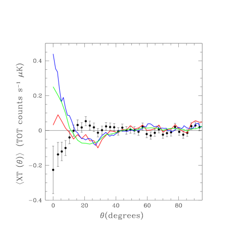
Figure 6: The earlier observations using the four year COBE data showed much less correlation, apparently because of noise in the maps. The correlation seen with WMAP (blue), is suppressed when WMAP is smoothed with the COBE beam (green); however, it is still much higher than the correlation with observed with COBE (red). While (COBE - WMAP) should be consistent with noise, it is apparently anti-correlated with the X-ray background (points with error bars). The reasons are unclear, but could indicate a low level systematic in the COBE data.

Furthermore, it is quite possible that the $COBE$ map contains some unknown, low amplitude systematic structure. The $CCF$ of the X-ray map with the difference of the $COBE$ and smoothed combination $WMAP$ maps is shown in Figure 6. It is clear from the plot that there is some systematic difference between the two CMB maps on angular scales $\mathrel{\raise 1.50696pt\hbox{$\scriptstyle<$}\kern-6.00006pt\lower 1.72218pt\hbox{{$\scriptstyle\sim$}}}10$ degrees. Dividing this $CCF$ by the $rms$ fluctuations of the X-ray map gives an indication of the correlated differences between the two CMB maps, i.e., $CCF/\sigma_{x}\sim 1$ to $2~{}\mu K$ compared to the $71~{}\mu K$ instrument noise per pixel in the COBE map. This level of discrepancy would have gone unnoticed in previous comparisons of the two maps. However, it is not possible to determine whether the discrepancy is due to such a systematic or is simply “unlucky” but statistically possible noise fluctuations in the COBE map. In any case, we are led accept the more statistically significant result with the much cleaner $WMAP$ data set presented here.

9 Conclusions

We conclude that the integrated Sachs-Wolfe effect has been detected at the $\sim 3~{}\sigma$ level. There is considerable evidence that the detection is not due to spurious systematics or contamination by point radio sources. If so, then these and possibly other recent observations (Boughn& Crittenden 2004; Nolta, et al. 2004; Myers et al. 2004; Fosalba & Gaztanaga 2004; Scranton et al. 2003; Afshordi, Loh,& Strauss 2004 ) offer the first direct glimpse into the production of CMB fluctuations and provide important, independent confirmation of the new standard cosmological model: an accelerating universe, dominated by dark energy. It should be pointed out that measurements of the power spectrum of CMB fluctuations do not show evidence of increased power on large angular scales ($\theta>20^{\circ}$) as predicted by the ISW effect, but rather indicate that there may be power missing on large angular scales (Spergel et al. 2003). This deficit is intriguing and may be telling us something about the formation of the very largest structures in the universe. The consequences of the ISW effect reported in this letter are primarily on smaller angular scales and are not in direct conflict with the larger angular scale power deficit.

ACKNOWLEDGMENTS

We thank Ed Groth and Greg Koehrsen for a variety of analysis programs and Bob Nichol for useful conversations. We acknowledge the use of the Legacy Archive for Microwave Background Data Analysis (LAMBDA). Support for LAMBDA is provided by the NASA Office of Space Science.

APPENDIX A

Here we briefly derive Equation 3 for the probability distribution of the product of two correlated Gaussian distributions. We begin by assuming that we have two Gaussian variables, $x$ and $y$, with unit variance and zero mean, and are described by the probability distribution:

$$P(x,y)=\frac{1}{(2\pi)\,\det|\tilde{C}|^{1/2}}\exp\left[-\frac{1}{2}(x,y)\tilde{C}^{-1}(x,y)^{T}\right].$$ (5)

The dimensionless correlation is given by the variable $c=\langle xy\rangle$, and the corresponding covariance matrix is

$$\tilde{C}=\left(\begin{array}[]{cc}1&c\\ c&1\end{array}\right).$$ (6)

The distribution of the product $z=xy$ is given by the marginalization of the distribution given the constraint:

$$P(z=xy)=\int_{-\infty}^{\infty}dx\int_{-\infty}^{\infty}dy\,\delta(xy-z)\,P(x,y).$$ (7)

Rewriting the Dirac delta function, $\delta(xy-z)=1/x\,\delta(y-z/x)$ if $x>0$, we can perform the $y$ integral, leaving:

$$P(z)=2\int_{0}^{\infty}\frac{dx}{x}P(x,z/x).$$ (8)

Substituting the above form for the two-dimensional distribution function, we find

$$P(z)=\int_{0}^{\infty}\frac{dx}{x}\frac{1}{\pi(1-c^{2})^{\frac{1}{2}}}\exp\left[-\frac{1}{2}(x^{2}-2cz+\frac{z^{2}}{x^{2}})/(1-c^{2})\right]$$ (9)

which can be rewritten as

$$P(z)=\frac{e^{cz/(1-c^{2})}}{\pi(1-c^{2})^{\frac{1}{2}}}\int_{0}^{\infty}\frac{dx}{x}\exp\left[-\frac{1}{2}(x^{2}+\frac{z^{2}}{x^{2}})/(1-c^{2})\right].$$ (10)

If we make the substitutions $x=e^{t}$ and $z^{2}=e^{2t_{0}}$, the integral can be written as

$$P(z)=\frac{e^{cz/(1-c^{2})}}{\pi(1-c^{2})^{\frac{1}{2}}}\int_{-\infty}^{\infty}dt\exp\left[-\frac{1}{2}(e^{2t}+e^{2t_{0}-2t})/(1-c^{2})\right].$$ (11)

Finally, defining $t^{\prime}=2t-t_{0}$, the final probability distribution can be found:

$$P(z) = \frac{e^{cz/(1-c^{2})}}{\pi(1-c^{2})^{\frac{1}{2}}}\int_{-\infty}^{\infty}\frac{dt^{\prime}}{2}\exp\left[-\cosh(t^{\prime})|z|/(1-c^{2})\right]$$ (12)

$$= \frac{e^{cz/(1-c^{2})}}{\pi(1-c^{2})^{\frac{1}{2}}}K_{0}\left(|z|/(1-c^{2})\right),$$ (13)

where $K_{0}$ is the modified Bessel function. (In evaluating the final integral, we have used Eqn. 3.337, Gradshteyn & Ryzhik 1980.)

References

- [1] Allen, J. Jahoda, K. & Whitlock, L. 1994, Legacy, 5, 27
- [2] Afshordi,N., Loh. Y.S.,& Strauss, M. A. 2004, PRD 69, 083524
- [3] Bahcall, N. Ostriker, J.P., Perlmutter, S. & Steinhardt, P., 1999, Science 284, 1481
- [4] Bauer, F. E., et al.2002, AJ, 124,2351.
- [Bennett et al.(2003)] Bennett, C. L. et al. 2003, ApJ Supp., 148,1.
- [5] Benson, A. J., Cole, S., Frenk, C.S., Baugh, C. M., & Lacey, C. G. 2000, MNRAS 311, 793.
- [6] Boldt, E. 1987, Phys. Rep., 146, 215
- [7] Boughn, S. 1998, ApJ, 499, 533
- [8] Boughn, S. 1999, ApJ, 526, 14
- [9] Boughn, S. & Crittenden, R. 2002, PRL 88, 1302
- [Boughn & Crittenden(2004a)] Boughn, S. & Crittenden, R. 2004a, Nature, 427, 45.
- [Boughn & Crittenden(2004b)] Boughn, S. & Crittenden, R. 2004b, ApJ, in press.
- [10] Boughn, S., Crittenden, R., & Koehrsen G. 2002, ApJ, 580, 672.
- [11] Boughn, S., Crittenden, R. & Turok, N. 1998, New Astron., 3, 275
- [12] Brinkmann, W., et al. A & A, 356,445.
- [Cowie et al.(2003)] Cowie, L., Barger, A., Bautz, M., Brandt, W., & Garmire, G. 2003, ApJ, 584, L57.
- [13] Ciliegi, P., et al. 2003, MNRAS, 342, 575.
- [14] Crittenden, R. & Turok, N. 1996, PRL 76, 575
- [15] Croom, S. et al. 2003, astro-ph/0310533
- [16] Fosalba, P., & Gaztanaga, E. 2004, MNRAS, 350, L37
- [17] Fry, J.N., 1996, ApJ 461, L65
- [18] Georgakakis, A., et al. 2003, MNRAS, 345, 939.
- [19] Gradshteyn, I.S., & Ryzhik, I.M., 1980, Table of Integrals, Series and Products, (Academic Press : New York), p 309.
- [20] Jahoda, K. 1993, Adv. Space Res., 13 (12), 231
- [21] Jahoda, K. & Mushotzky, R. 1989, ApJ, 346, 638
- [22] Kamionkowski, M. 1996, PRD 54, 4169
- [23] Kinkhabwala, A. & Kamionkowski, M. 1999 Phys. Rev. Lett. 82, 4172
- [24] Myers, A.D., Shanks, T., Outram, P. J. & Wolfendale, A.W. 2004, MNRAS, 347, L67
- [25] Nolta, M.R. et al. 2004, ApJ, 608, 10
- [26] Piccinotti, G., et al. 1982, ApJ, 253, 485
- [27] Reich, W., et al., 2000, A & A, 363, 141.
- [28] Riess, A., et al. 2004, ApJ, 607, 665.
- [29] Sachs, R. K. & Wolfe, A. M. 1967, Ap J, 147, 73.
- [30] Scranton, R. et al. 2003, astro-ph/0307335
- [31] Spergel, D. N. et al. 2003, ApJS, 148, 175
- [32] Steffen, A., Barger, A., Cowie, L., Mushotzky, R., & Yang, Y. 2003, ApJ, 596, L23
- [33] Tegmark, M., de Oliveira-Costa, A. & Hamilton, A., 2003, PRD 68, 123523
- [34] Tegmark, M. & Peebles, P. J. E. 1998, ApJ, 500, L79
- [35] Voges, W. et al. 1996, IAU Circ., 6420, 2
- [36] Wake, D. A. et al. 2004, ApJ610, L85
- [37] White, R. & Stemwedel, S. 1992, Astronomical Data Analysis Software and Systems I, eds. D. Worrall, C. Biemesderfer & J. Barnes (San Francisco: ASP), 379