The Capodimonte Deep Field

We present the Capodimonte Deep Field (OACDF), a deep field covering an area of 0.5 $\deg^{2}$ in the $B$, $V$, $R$ optical bands plus six medium-band filters in the wavelength range 773–913 nm. The field reaches the following limiting magnitudes: $B_{AB}\sim 25.3$, $V_{AB}\sim 24.8$ and $R_{AB}\sim 25.1$ and contains $\sim$ 50000 extended sources in the magnitude range 18 $\leq R_{AB}\leq$ 25.0. Hence, it is intermediate between deep pencil beam surveys and very wide but shallow surveys. The main scientific goal of the OACDF is the identification and characterization of early-type field galaxies at different look-back times in order to study different scenarios of galaxy formation. Parallel goals include the search for groups and clusters of galaxies and the search for rare and peculiar objects (gravitational lenses, QSOs, halo White Dwarfs). In this paper we describe the OACDF data reduction, the methods adopted for the extraction of the photometric catalogs, the photometric calibration and the quality assessment of the catalogs by means of galaxy number counts, spectroscopic and photometric redshifts and star colors. We also present the first results of the search for galaxy overdensities. The depth of the OACDF and its relatively large spatial coverage with respect to pencil beam surveys make it a good tool for further studies of galaxy formation and evolution in the redshift range 0–1, as well as for stellar studies.

1 Introduction

Wide and deep surveys are a vital tool in modern astronomy: they provide the large datasets of objects needed (both at high and low redshifts) to improve our knowledge of the physical mechanisms driving galaxy formation and evolution.

Recent wide field surveys, such as DPOSS, 2MASS, SDSS and 2DF, (Djorgovski et al. 2000, Colless et al. 2001; Jarrett et al. 2000; York et al. 2000) provide an unprecedented wealth of information on the structure of the local Universe.

On the other hand, the complementary pencil beam deep surveys (i.e. relatively small patches of the sky observed in several bands with high angular resolution and high S/N ratios at faint magnitude levels) allow us to investigate the high-$z$ Universe ($z\gtrsim 1$), providing large sets of distant galaxies to constrain the different evolution scenarios.

In the past, the significance of deep fields was limited by the constraints of the small field of view covered by single CCD detectors and the need to obtain large fractions of observing time with 4 m class telescopes. The small spatial coverage of the first studies (Tyson 1988, Lilly et al. 1995; Ellis et al. 1996; Le Fevre et al. 1996) succeeded in tracing only a rough and broad picture of galaxy evolution in the redshift range $0<z<0.8$ and therefore did not allow strong constraints on the various scenarios proposed for galaxy formation and evolution (White and Frenk 1991; Cole et al. 2000; Aragon-Salamanca et al. 1998; Peebles 2002).

The Hubble Deep Fields (e.g. Ferguson, Dickinson & Williams 2000) has marked a cornerstone in our understanding of galaxy evolutionary processes, providing unprecedented contraints on the theoretical scenarios for galaxy formation and evolution.

Similar deep surveys have been recently performed using ground-based telescopes of the 10m class generation: the Subaru Deep Field (Maihara et al. 2001), the Fors Deep Survey (Heidt et al. 2003) and the Gemini Deep Deep Survey (Abraham et al. 2004). However, an important drawback of these deep surveys is that the typical field of view has angular sizes at $z\sim 1$ which are relatively small with respect to the scales relevant for large-scale structure. Thus, in order to study the properties of distant galaxies at high redshift in different large scale enviroments, it is mandatory to control field-to-field variations, by means of deep surveys along many different lines of sight or extended to larger contiguous sky areas.

The advent of wide field imagers on dedicated survey telescopes, like the wide-field imager (WFI) at the ESO/MPG 2.2m telescope, allow one to perform deep surveys on sky areas of the order of 1 square degree, thus providing an ideal tool to gather high accuracy data for statistically significant samples of objects in the redshift range $0<z<1$. This has prompted the observation of several deep fields at optical and near infrared wavelengths: COMBO-17 (Wolf et al. 2003); K20 (Cimatti et al. 2002), MUNICS (Drory et al. 2001), the VIRMOS-VLT deep field (Le Fevre et al. 2003; Mc Cracken et al. 2003; Radovich et al. 2004).

While these surveys cannot, in general, compete with the HDFS and the 10m class telescope deep surveys in terms of depth, they allow one to study in detail the galaxy population up to $z\simeq 1$ in a much larger field of view.

This fact is extremely important, for instance, when determining the luminosity function and its possible evolution up to $z\simeq 1$ (e.g., Wolf et al. 2003).

In 1999, the Osservatorio Astronomico di Capodimonte (INAF-OAC) started the Capodimonte Deep Field (OACDF) project using WFI at the ESO/MPG 2.2m telescope at La Silla, Chile. The OACDF covers an area of 0.5 $\deg^{2}$ in the $B$,$V$, $R$ optical bands and in six medium-band filters in the wavelength range 773–913 nm. The OACDF is intermediate between deep pencil beam surveys and very wide, but shallow surveys. As it will be shown in the following paragraphs the OACDF reaches limiting magnitudes $B_{AB}\sim 25.3$, $V_{AB}\sim 24.8$ and $R_{AB}\sim 25.1$ and contains $\approx$ 50000 extended sources in the magnitude range 18 $\leq R_{AB}\leq$ 25.0.

The OACDF was complemented with a first spectroscopic follow-up and with a shallow photometric survey overlapping the deep survey and covering 1 $\deg^{2}$ in the $B$,$V$, $R$ and $I$ bands. The shallow survey reaches a depth of $I_{AB}\sim 22.1$ and was planned in order to enhance the statistics at low redshift.

The OACDF observing strategy was driven mainly by the identification and characterization of a statistically significant sample of early-type galaxies at different redshifts and in different environments. The number density, as well as the global morphological and photometric properties of these objects, are predicted to vary for different formation scenarios (Aragon Salamanca et al. 1998, Kauffmann & Charlot 1998, Somerville et al. 2004). The filter set-up and in particular the availabilty of medium band filters in the range 753-913 nm, allow us to trace the D4000 break over the redshift range from 0 to 1 and therefore to obtain an accurate estimate of the photometric redshifts for these objects.

Parallel goals of the OACDF project are:

• the search for groups and clusters of galaxies to study the luminosity function of galaxy clusters, as well as their luminosity and color segregation, both linked to the more general question of the evolution of galaxies in environments with different densities (Menanteau et al. 1999). Another aspect is to study the cluster morphology (clustering and sub-clustering) which bear relevant information on the history of the Universe (Navarro, Frenk and White 1996). The identification of a sample of groups of galaxies and intermediate-richness clusters of galaxies at intermediate redshift, extracted in a homogeneous way, is necessary to study the properties of galaxies in moderately dense environments.

• the search for rare/peculiar objects, in particular gravitational lenses and high-redshift QSOs (z$>$3);

• the identification of nearby galaxies with strong emission lines using the medium-band filters to perform clustering and correlation function studies.

• to provide a photometric and astrometric database for stellar studies.

While some peculiar objects present in the OACDF have already been discussed elsewhere (cf. gravitational lenses in Sazhin et al. 2003; white dwarfs in Silvotti et al. 2003), in this paper we present the OACDF photometric calibration, the catalog extraction, the quality assessment of the photometric catalogs through the derivation of galaxy number counts, spectroscopy of stars and galaxies by means of photometric and spectroscopic redshifts. We also present the first results of the search for galaxy overdensities.

In a forthcoming paper, we will use the OACDF data, the photometric redshift determinations and the available spectra in order to analyze the redshift and environmental evolution of scaling-laws, such as the Kormendy relation (Kormendy 1977, Ziegler et al. 1999, La Barbera et al. 2003), and of the stellar populations of these objects through the use of the Lick indices (Faber et al. 1985, Worthey et al. 1992) and stellar population synthesis models (Thomas et al. 2003).

Other future OACDF papers will include the following tasks:

• search for groups and clusters of galaxies: in the present paper we describe the adopted methods for the detection of groups and clusters of galaxies in the OACDF (see Section 6). In a future paper we will use the candidate clusters as part of a larger statistical sample needed to derive the multiplicity function and to study the luminosity function as a function of the environment. Follow-up spectroscopic studies are in course.
  

• search for Gravitational lenses: an important by-product of a survey like the OACDF is the possible detection of strong gravitational lenses (GLs). We have therefore started an extensive search for GLs in the OACDF2 and OACDF4 fields by spectroscopic observations at the ESO 3.6m telescope at La Silla, Chile. In a future paper we will present the methodology and the results of this search and, in particular, its implications for wider surveys with VST, which will allow us to discover several tens of bright GLs in the Southern emisphere.
  

• the spectroscopic confirmation of white dwarf (WD) candidates selected through their colors. Spectroscopic data were obtained at the ESO NTT and 3.6m telescopes and are under reduction; some preliminary results are shown in Silvotti et al. (2003). The main goal of this project is to increase the WD statistics, in particular for the cooler, fainter and older objects, which contain crucial information on the genesis of our Galaxy: age of the galactic disk (and halo) through the WD luminosity function, initial mass function, and stellar formation rate (see Fontaine et al. 2001 for an updated review). Of particular interest is the halo WD population as these rare and faint objects, whose statistics are almost totally unknown, might partially contribute to the galactic dark matter. This is suggested by the results of the MACHO+EROS microlensing experiments which show that microlensing events are mainly produced by halo objects with an average mass of $\sim$0.5 M_⊙ (Alcock et al. 2000).

The present paper is structured as follows: in Section 2 we present the field selection and the observational strategy for the imaging and initial spectroscopic follow-up. The data reduction and photometric calibration, as well as the systematic behavior of the zero points of the ESO-WFI CCDs, and the spectroscopic data reduction are reported in Section 3. In Section 4 we discuss the problems posed by catalog extraction, while the quality assessment of the OACDF catalogs are discussed in Section 5. First results on the search for groups and clusters of galaxies are reported in Section 6 and a summary is presented in Section 7. Finally, the Appendix reports a catalog containing magnitudes and spectroscopic redshifts for 114 galaxies observed in our first spectroscopic follow-up. The catalog also contains the magnitudes and spectral types for 59 stars in the OACDF.

2 Field selection and observations

The central coordinates ($\alpha$(2000)$\approx$12:25:10, $\delta$(2000)$\approx$-12:48:31) of the OACDF were selected in order to identify a field matching the following criteria:

• lack of sources brighter than $V=9$ mag to minimize CCD saturation and ghost effects;

• high galactic latitude to avoid high stellar crowding;

• low interstellar (IS) extinction ($E(B-V)<$0.03 mag) according to the Burstein and Heiles (1982) maps;

• to be observable from both hemispheres to have the possibility of performing follow-ups using telescopes at several sites.

The observations were carried out in three different periods (18–22 April 1999, 7–12 March 2000 and 26–30 April 2000), using the Wide-Field Imager (WFI) CCD mosaic camera (Baade et al. 1998) at the ESO/MPG 2.2m telescope at La Silla in Chile. This camera consists of eight 2k$\times$4k CCDs forming a 8k$\times$8k array with a scale of $0.238^{\prime\prime}$/pix.

In the shallow survey, four adjacent $30^{\prime}\times 30^{\prime}$ fields (hereafter OACDF-1 through 4) covering a $1^{\circ}\times 1^{\circ}$ field in the sky were observed in the $B$, $V$, $R$ and $I$ bands (see Table 1 for the coordinates of the centers of the $4$ fields). The OACDF2 and OACDF4 were also selected for the 0.5 deg² deep survey, performed in the $B$, $V$, $R$ broad-bands and in the $\lambda$753, $\lambda$770, $\lambda$791, $\lambda$815, $\lambda$837, $\lambda$884 and $\lambda$914 medium-band filters.

For the shallow survey, each field was observed in $5$ ditherings, while at least 8 ditherings were obtained for the deep survey, the exact number depending on the band. The adopted dithering pattern is that described in the ESO-WFI observers guide (Brewer and Agustein 2000). A detailed summary of the observations is provided in Table 2.

Table 1: Coordinates of the OACDF centers.

Field	$\alpha$(2000)	$\delta$(2000)
OACDF1	12  26  20.4	-12  30  20
OACDF2	12  24  27.0	-12  30  20
OACDF3	12  26  20.4	-13  01  20
OACDF4	12  24  27.4	-13  01  20

Table 2: Summary of the OACDF observations.

Field	obs. run	Filter	# diths	Total exp.	Seeing	Airmass	Zero points	Col.Terms
				time	arcsec		$ZP^{\dagger}$
OACDF2 deep	1st	$B$	12	2.0h	1.24	1.287	24.77	$+$0.24
OACDF2 deep	1st	$V$	10	1.7h	1.07	1.184	24.30	$-$0.14
OACDF2 deep	1st	$R$	13	3.3h	1.11	1.482	24.63	$-$0.03
OACDF2 deep	1st-2nd	753nm	9+10	6.5h	0.88	1.512	21.95
OACDF2 deep	1st-2nd	770nm	9+10	6.0h	0.86	1.544	21.88
OACDF2 deep	1st-2nd	790nm	9+10	6.5h	0.99	1.084	21.80
OACDF2 deep	1st-2nd	815nm	9+9	6.8h	0.79	1.044	21.59
OACDF2 deep	1st-2nd	837nm	9+8	6.6h	0.95	1.468	21.54
OACDF2 deep	1st-2nd	914nm	10+10	5.6h	0.90	1.046	21.15
OACDF4 deep*	3rd	$B$	8	2.0h	0.99	1.095	24.76	$+$0.22
OACDF4 deep	2nd-3rd	$V$	7	1.8h	0.95	1.042	24.23	$-$0.18
OACDF4 deep	2nd-3rd	$R$	4+14	4.2h	0.99	1.410	24.54	$-$0.03
OACDF4 deep	2nd-3rd	753nm	5+10	4.8h	0.95	1.042	21.81
OACDF4 deep	3rd	770nm	7	2.1h	1.33	1.250	21.72
OACDF4 deep	3rd	790nm	9	3.0h	0.95	1.380	21.65
OACDF4 deep	2nd-3rd	815nm	5+6	3.5h	0.95	1.110	21.42
OACDF4 deep	3rd	837nm	7	3.3h	1.20	1.100	21.44
OACDF4 deep	3rd	914nm	9	2.5h	0.81	1.110	21.05
OACDF shallow	1st	$B$	5	20min	0.86	1.078	24.77	$+$0.24
OACDF shallow	1st	$V$	5	10min	0.83	1.237	24.30	$-$0.14
OACDF shallow*	2nd	$R$	5	10min	1.38	1.320	24.45	$-$0.03
OACDF shallow	1st	$I$	5	10min	0.81	1.650	23.31	$+$0.12

$\dagger$ The reported zero points are those for the first and third observing runs, as the second run was partially non-photometric.

* Due to technical problems it was not possible to calibrate the $B$-band during the third run. Stars on the OACDF4, calibrated during the first observing run, were used as secondary standards. A similar procedure was applied to the shallow $R$-band images of the second run.

The standard fields L 98, L 104, L 107, L 110 and PG 1525, selected from the Landolt (1992) equatorial regions, were observed to perform the broad-band photometric calibration. Likewise, the spectrophotometric standard stars EG 274, Hill 600, LTT 3864, LTT 4364, LTT 6248, and LTT 7379 were observed in the medium-band filters for absolute flux calibration purposes. Typically, each standard field was observed twice.

2.1 Spectroscopic observations

The first spectroscopic follow-up of the OACDF was performed in April 2000 using the ESO Multi-Mode Instrument (EMMI) at the New Technology Telescope (NTT) in the multi-object spectroscopy (MOS) mode. The selection criteria for the observed objects will be published in our forthcoming paper on the identification and characterization of early-type galaxies in the OACDF. In this paper we report the observations and use the spectra to fine-tune the software parametrization for the photometric redshift determinations and for quality assessment.

Five 9 x 4 arc-min² fields distributed in the OACDF2 were observed through grism No. 3, which yields a dispersion of 2.3 Å/pix. Some ten flat-field exposures were taken nightly. Before and after the science spectra, HeAr spectra were observed in each configuration and mask for wavelength calibration purposes. Given the faint magnitude of the targets, the pixels in the dispersion direction were re-binned by a factor of two to minimize the noise. The resulting nominal resolution was about 10 Å (FWHM) and the covered spectral range was from about 3800 Å to about 8800 Å, but the resulting spectral range for each individual object depends on the position of each individual slit relative to the edges of the mask. To remove cosmic ray hits and increase the S/N ratio, three science exposures of 40 minutes each were made, amounting to a total of 2 hours of exposure per field. Three acquisition images, useful for the selection of the slit positions, were obtained by the NTT team prior to the observations. The other three acquisition images were obtained during the first observing night. Typically 35 slits per mask were used. Three apertures were normally assigned to bright stars for mask alignment purposes. The spectrophotometric standard stars Hil600 and Eg274 were observed with the same instrumental set-up as the objects for flux calibration.

3 Data reduction

3.1 Imaging

Data reduction was performed using the task mscred in IRAF. Bias correction, super-flat-fielding and fringing correction were done on a nightly basis.

For each dithering sequence we chose a reference exposure and computed the astrometric solution for the CCDs in that exposure with reference to an external astrometric catalog. A polynomial fit was then performed between the source positions in the reference CCD and those in the other exposures. As reference astrometric catalogue we use the USNO–A2 catalog (Monet et al. 1998) which allows to achieve an absolute RMS accuracy $\sim$ 0.3”. In order to improve the internal astrometric precision we first used the USNO–A2 catalog as a reference for the R-band and the resulting catalog, extracted from the R-band stacked image, was then used as reference catalog for the pointings in the other bands. The internal RMS accuracy between source positions in different bands is less than 0.1”. In order to correct for transparency variations we also selected a reference image and normalized the others to the same flux level, using sources in the overlap regions. Finally, images were re-sampled, scaled in flux and co-added using the average sigma clip. More details in the WFI data reduction are provided in Alcalá et al. (2002).

3.1.1 The photometric calibration

The broad-band photometric calibration to the Johnson-Cousins $BVR_{C}I_{C}$ system was performed using the standard Landolt (1992) fields. For the field Landolt-98, we used the larger set of photometric standards by Stetson (2000). Photometric calibrated magnitudes and instrumental magnitudes are related by the following equations:

$$B=b+C_{B}\cdot(B-V)+Z_{B},$$ (1)

$$V=v+C_{V}\cdot(B-V)+Z_{V},$$ (2)

$$R_{C}=r+C_{R}\cdot(V-R_{C})+Z_{R},$$ (3)

$$I_{C}=\leavevmode\nobreak\ i\leavevmode\nobreak\ +C_{I}\cdot(V-I_{C})+Z_{I},$$ (4)

where $b,v,r,i$ are the instrumental magnitudes corrected for atmospheric extinction, $C_{B},C_{V},C_{R},C_{I}$ the color terms and $Z_{B},Z_{V},Z_{R},Z_{I}$ the zero points. We used the mean extinction coefficients for the La Silla observatory .

Figure 1: Left: relative photometric offsets versus the CCDs for the broad-band filters (upper panel). The different line types represent the different observing dates as labeled. The average over the broad-band filters is shown in the lower panel. Right: the same but for the medium-band filters.

Photometric calibrations were achieved using a number of stars ranging from $100$ to $200$. The fit residuals are typically less than 3%, but in some cases the residuals are as high as 5%. The relatively high residuals may be a consequence of the non-uniform background illumination over the field of view, that will be discussed in Section 3.2. A few points with particularly high residuals are due to stars partially falling in the CCD gaps and/or to photometric/astrometric errors in the standard catalog. Aberrant points were rejected by a sigma clipping algorithm. Points typically above the 2$\sigma$ level were not used for the calibration.

The photometric zero points and the corresponding color terms are listed in Table 2. Since the second run was partially non-photometric, we give in Table 2 only the zero points of the first and third observing runs. Also, due to technical problems, it was not possible to calibrate the $B$-band of the field OACDF4 during the third observing run. The latter calibration was done using secondary standard stars in the OACDF. A similar approach was adopted for the shallow observations of the second observing run in the $R$-band.

The flux calibration for the medium-band observations was performed using spectrophotometric standard stars. These calibrations provide AB magnitudes. The detailed explanation of the medium-band filter calibrations, as well as the determination of AB magnitudes can be found in Alcalá et al. (2002).

For practical purposes, we transform our broad-band instrumental WFI magnitudes into AB magnitudes using the following expressions:

$$B_{AB}=b+Z_{B}-0.093,$$ (5)

$$V_{AB}=v+Z_{V}+0.002,$$ (6)

$$R_{AB}=r+Z_{R}+0.215,$$ (7)

$$I_{AB}=\leavevmode\nobreak\ i\leavevmode\nobreak\ +Z_{I}+0.509$$ (8)

In the catalog presented in the appendix, AB magnitudes are given (Tables 6 and 7).

In order to check the photometric homogeneity over the eight CCDs and its dependence on the star color (Manfroid and Selman 2001; Monelli et al. 2003), we also observed a few selected standard fields in each of the eight CCDs. For the broad-band filters, we used the Landolt field PG1525-071, which contains five stars with $(B-V)$ colors ranging from -0.198 to 1.109. For the medium-band filters we used the spectro-photometric standards Eg 274, Hill 600 and LTT 6248. We find no color dependence as well as no time dependence but, on the other hand, we find an offset of the instrumental magnitude among the eight CCDs. The effect is summarized in Figure 1, where we show the fluxes of the standard stars measured in each CCD, relative to the mean value over the 8 CCDs. Within the errors, the trend is the same in the different bands ($B$, $V$, $R$, $I$) and at different times (from April 1999 to April 2000). As stressed by the above quoted authors this photometric offset may be attributed to an additional light pattern caused by internal reflections of the telescope corrector. Such a pattern, with an amplitude that depends also on the exposure time, is present in each image (including flat-fields) and must be corrected before flat-fielding. In order to correct for this effect in a proper way, one should know the additional-light pattern.

The photometric offset appears to be slightly stronger in the medium-band filters than in the broad-band ones (see Figure 1 right panel). We find an offset in the flux of the stars which may introduce an average uncertainty of $\pm$3% in the broad-band $B$, $V$, $R$, $I$ filters and of $\pm$5% in the medium-band filters.

3.2 Spectroscopy

The MOS data reduction was performed using the MIDAS package following standard reduction techniques for multi-object slit spectroscopy. For each configuration or mask, the reduction consisted of the bias subtraction, definition of slit positions, flat-fielding, row-by-row wavelength calibration, background subtraction, extraction of one-dimensional spectra and relative flux calibration.

For each mask or field, the reduction steps were the following:

i) the average bias frame was subtracted from all the frames and a master flat-field was determined using the median option within MIDAS;

ii) the definition of the slit positions (along the direction perpendicular to the dispersion) and the flat-fielding were performed using the master flat and the context MOS within the MIDAS environment;

iii) the three multi-spectra frames of each field were combined using a sigma clipping algorithm for the rejection of cosmic ray hits;

iv) for each configuration or mask, the individual two-dimensional long-slit spectra were extracted from the combined multi-spectra frames. The next steps were then performed following the standard pipeline of the context ”long” within the MIDAS package;

v) a row-by-row wavelength calibration was done on each individual two-dimensional long-slit spectrum using its corresponding HeAr comparison spectrum, extracted exactly in the same way as the science spectrum;

vi) the background subtraction was then performed and the one-dimensional spectra were extracted;

vii) the spectra of the flux standards, reduced in the same way as the science spectra, were then used for the determination of a mean response function. A response function was determined for each one of the two observing nights. Finally, a relative flux calibration was then performed on the one-dimensional spectra by applying the corresponding response function.

4 Source extraction from the WFI images

Catalog extraction was performed using SExtractor (Bertin and Arnouts 1996). In order to ”increase” the signal–to–noise ratio, the images are filtered with a kernel that, in our case, is a Gaussian with a constant FWHM that properly matches the seeing on the images. The source detection is performed on the filtered image and the detection threshold is determined as the best compromise between limiting magnitude and percentage of spurious detections.

The photometry was also performed with SExtractor. Magnitudes were measured both in fixed circular or CORE apertures (2$\sigma$ and 3$\sigma$ of the PSF FWHM) and in Kron-like (1980) elliptical apertures (MAG_AUTO in SExtractor, cf. Bertin and Arnouts 1996).

MAG_AUTO provides the best measurement of the object total flux because the elliptical aperture is adaptively determined from the object dimensions. However, in the case of blended objects MAG_AUTO does not provide reliable results. In these cases (indeed representing a very low percentage of the total catalogue), we use the CORE aperture photometry.

We also use the MAG_AUTO magnitudes to measure objects colors, except in the case of blended sources in which CORE aperture magnitudes are used.

Table 3: Completeness magnitudes vs. wavelengths.

S/N	$B_{AB}$	$V_{AB}$	$R_{AB}$	753	770	791	816	837	915
10	24.6	24.0	24.3	22.8	22.4	22.1	22.5	21.8	21.9
5	25.3	24.8	25.1	23.7	23.3	23.0	23.4	22.7	22.8

4.1 Completeness magnitude limit of the OACDF

The best parameter set for the catalog extraction were determined, for each final stacked image, using a series of Monte Carlo simulations. The goal was: i) to determine the completeness limit of the extracted catalogs, and ii) to estimate of the fraction of spurious detections (see Arnaboldi et al. 2002 for details).

We ran a series of simulations by randomly adding a synthetic population of point-like sources with a known luminosity fuction (LF) and positions. The completeness limit, i.e. the magnitude at which 50% of the input catalog is lost, was then recovered by matching the extracted catalog with the modelled population. This procedure allowed us to derive the completeness limit of $25.1$ AB mag for the $R$-band mosaic (see Figure 2). The completeness limits for the OACDF at S/N ratios of 10 and 5 in the different bands are listed in Table 3.

Figure 2: Magnitude distributions in the $R$-band mosaic. The simulated sample, connected by the dotted line, is represented with squares, while the extracted sample is represented with triangles. The solid line represents the magnitude distribution of the modeled sample.

In order to estimate the fraction of spurious detections we proceeded as follows: a simulated image was built from the background interpolated by SExtractor, by adding the noise map constructed by multiplying the SExtractor RMS map by a Gaussian noise image with null mean and $RMS=1$. For a given SExtractor parameter set, the number of spurious detections was then determined as the difference between the SExtractor catalog and the matched catalog with the input modelled population. For the OACDF $R$-band mosaic, we find that the number of spurious sources, relative to the total number of detected objects, is less than 2% at the completeness limit of 25.1 AB mag.

Besides the usual problems posed by the bright (saturated) stars which produce a large number of spurious objects in their extended halos, mosaic images pose additional problems in the regions at the edges of the individual images which have lower S/N due to the dithering. The usual approach would have been to mask out these regions, keeping track of their size and position to correct the final statistics. However, so as not to lose completely the information on the objects falling in such regions, a flag was introduced in the catalogues as follows: we flag as “BAD” those objects having either high background values (i.e. objects in proximity of saturated objects) or high background RMS values (i.e. mostly border objects). The threshold to activate such flag was optimized on a trial and error basis via the accurate inspection of objects flagged as spurious. Extensive testing showed that the best compromise was achieved by setting such treshold at either 5 times the value of the local background images and/or at a local RMS 20% larger than the average RMS of the mosaic itself. These criteria assume that the catalogs have been extracted from background subtracted images.

4.2 Star–galaxy separation

To distinguish point-like sources from extended ones we use the SExtractor parameter CLASS_STAR. Star/galaxy classification in SExtractor is made using neural networks trained on simulated galaxies on single CCD images and is mainly based on the deviations of extended objects from a well behaved PSF. We use different CLASS_STAR indexes for the different bands. We set CLASS_STAR equal to 0.95, 0.98 and 0.98 for the $B$, $V$ and $R_{C}$ bands respectively.

In mosaic images, the determination of the final PSF is usually non trivial due to the combined effects of ditherings and varying PSF among the single images. In order to test the reliability of the SExtractor CLASS_STAR parameter we use the spectra obtained for the sample of 173 objects (114 galaxies and 59 stars). In this sampe, the objects classified as stars by SExtractor are 63 with 5% contamination due to misclassified galaxies, while the objects classified as galaxies are 110 with no contaminants. Overall, the SExtractor classification turns out to be quite reliable in the magnitude range of the spectroscopic sample, ie. brighter than I=22.

Table 4: Source counts of the OACDF at each band.

AB mag.	logNB deg-2	logNV deg-2	logNR deg-2
17.0	0.90${}^{+0.23}_{-0.53}$	1.10${}^{+0.19}_{-0.33}$	1.46${}^{+0.13}_{-0.19}$
17.5	1.00${}^{+0.20}_{-0.37}$	1.38${}^{+0.13}_{-0.19}$	1.72${}^{+0.10}_{-0.13}$
18.0	1.35${}^{+0.14}_{-0.22}$	1.74${}^{+0.10}_{-0.13}$	2.11${}^{+0.07}_{-0.08}$
18.5	1.60${}^{+0.11}_{-0.16}$	2.10${}^{+0.07}_{-0.08}$	2.23${}^{+0.06}_{-0.07}$
19.0	1.77${}^{+0.09}_{-0.12}$	2.26${}^{+0.06}_{-0.07}$	2.56${}^{+0.04}_{-0.05}$
19.5	2.05${}^{+0.07}_{-0.08}$	2.62${}^{+0.04}_{-0.04}$	2.78${}^{+0.03}_{-0.03}$
20.0	2.26${}^{+0.06}_{-0.07}$	2.81${}^{+0.03}_{-0.03}$	2.99${}^{+0.03}_{-0.03}$
20.5	2.42${}^{+0.06}_{-0.06}$	3.00${}^{+0.02}_{-0.03}$	3.17${}^{+0.02}_{-0.02}$
21.0	2.59${}^{+0.04}_{-0.04}$	3.17${}^{+0.02}_{-0.02}$	3.32${}^{+0.02}_{-0.02}$
21.5	2.86${}^{+0.03}_{-0.03}$	3.30${}^{+0.02}_{-0.02}$	3.48${}^{+0.02}_{-0.01}$
22.0	3.05${}^{+0.02}_{-0.02}$	3.49${}^{+0.01}_{-0.02}$	3.62${}^{+0.01}_{-0.01}$
22.5	3.29${}^{+0.02}_{-0.02}$	3.65${}^{+0.01}_{-0.01}$	3.77${}^{+0.01}_{-0.01}$
23.0	3.54${}^{+0.01}_{-0.01}$	3.86${}^{+0.01}_{-0.01}$	3.93${}^{+0.01}_{-0.01}$
23.5	3.79${}^{+0.01}_{-0.01}$	4.08${}^{+0.01}_{-0.01}$	4.10${}^{+0.01}_{-0.01}$
24.0	4.03${}^{+0.01}_{-0.01}$	4.26${}^{+0.01}_{-0.01}$	4.24${}^{+0.01}_{-0.01}$
24.5	4.21${}^{+0.01}_{-0.01}$	4.37${}^{+0.01}_{-0.01}$	4.34${}^{+0.01}_{-0.01}$
25.0	4.31${}^{+0.01}_{-0.01}$	4.35${}^{+0.01}_{-0.01}$	4.37${}^{+0.01}_{-0.01}$
25.5	4.41${}^{+0.01}_{-0.01}$	4.06${}^{+0.01}_{-0.01}$	4.34${}^{+0.01}_{-0.01}$

Figure 3: Comparison of the source number counts in the OACDF (filled circles) with those from the literature. The logarithmic counts are in half-magnitude bins, in the $B$, $V$, and $R$ bands (top, middle and bottom panels respectively) and are normalized to the OACDF deep survey area of 0.5 deg². The 1$\sigma$ Poissonian errors, also provided in Table 4, are shown.

5 Quality Assessment

In the following sub-sections we assess the quality of the OACDF catalogs by the comparison of the galaxy number counts with those in the literature and using the spectroscopic observations of stars and galaxies in the OACDF.

5.1 Source counts

In Figure 3 the number counts of galaxies in the OACDF, in the $B$, $V$, $R_{C}$ deep fields, are shown. Other number counts from the recent literature are also overplotted for comparison. The star/galaxy separation is done here on each single catalog by using the stellarity index from SExtractor, but without completeness correction applied. Despite this, there is a good agreement between the source number counts of the OACDF data and those from the literature.

The number counts (log N/0.5mag/deg^-2) per magnitude bin at each band are reported in Table 4. The magnitudes are AB magnitudes. The logarithmic counts are reported in half-magnitude bins, selected in the $B$, $V$, and $R$ bands, normalized to the effective area of the OACDF deep survey (0.5 deg²).

5.2 Spectroscopic redshifts

In order to determine spectroscopic redshifts the Ca II at $\lambda$3933.68 & $\lambda$3968.49 Å lines and the Mgb ($\lambda$5173 Å) absorption features, as well as the “G” band at $\lambda$4300 Å were identified and fitted with Gaussians for the central wavelength measurements. In order to further confirm the redshift determinations, a cross-correlation analysis was applied to the sample of galaxy spectra. For this purpose we used the fxcor task under IRAF. Several late type stars, obtained with the same instrumental set up, were used as templates for the cross-correlation analysis. Moreover, only parts of the spectra, not affected by telluric absorption lines, were considered. The typical error of the spectroscopic redshifts is around $\pm$0.005.

The total number of useful spectra is 173. The coordinates, AB magnitudes, redshifts and spectral types (see next Section) of these objects are listed in Tables 6,  7 and  8. 59 of these spectra resulted to be stellar objects. The remaining 114 objects are galaxies. For 24 of these, the redshift determination is uncertain because their S/N ratio is less than 10. We distinguish these objects in Table 8 with a question mark next to the redshift value.

5.3 Stellar spectral types

The stellar spectral types were determined by visual comparison of the stellar spectra with those of the grid of spectral standard stars taken from the library of stellar spectra by Jacoby et al. (1984). The most important spectral features considered for the spectral type classification were: Mg I $\lambda$5167, $\lambda$5173, and, whenever possible, the “G” band $\lambda$4300 for the G stars, the Ca I $\lambda$6162 and Fe I $\lambda$5227 for the late G and early K stars, the Na I $\lambda$5893 and the Fe I blend $\lambda$6495 for the K stars, and the TiO bands $\lambda$4954, $\lambda$5448, $\lambda$6159 for the late K and the M stars.

The magnitudes and spectral types of these stars are provided in Tables 6, 7 and 8. In order to transform the $B_{AB}$, $V_{AB}$, $R_{AB}$ and $I_{AB}$ magnitudes, reported in Table 6, into the Johnson-Cousins system, the transformation equations 9, 10, 11 and 12 given in the appendix, must be applied.

In Figure 4 the $(B-V)$ and $(V-I_{C})$ colors of the stars are plotted versus their spectral types. In these plots the relation between color versus spectral type, taken from the stellar library by Lejeune et al. (1997), is over-plotted as a continuous line. As can be seen, there is a good agreement of the spectral types and colors with those of the library of stellar spectra by Lejeune et al. (1997).

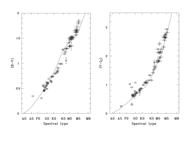
Figure 4: $(B-V)$ and $(V-I_{C})$ colors of the stars observed with EMMI-MOS versus their spectral type (circles in the left and right panels respectively). The continuous line represents the relationship between the corresponding colors and spectral type, taken from the stellar library by Lejeune et al. (1997).

As a further check, in Figure 5 we show the $(B-V)$ vs. $(V-R_{C})$ diagram of point-like sources (CLASS_STAR $>$ 0.85) in the OACDF. As expected, the colors are consistent with those expected for stars, which provides a further photometric check of the OACDF catalogs.

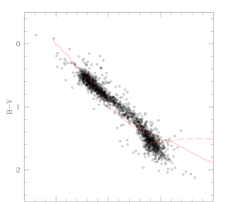
Figure 5: Color-color diagram for the objects classified as stars (open circles) using the criterium CLASS_STAR $>$ 0.85 for the sources detected in the $B$,$V$ and $R$ bands. The synthetic colors for dwarfs and giants, taken from the standard stellar library by Lejeune et al. (1997), are plotted with the continuous and dashed lines respectively.

5.4 Photometric redshifts

Photometric redshifts were determined using the HYPERZ package (see Bolzonella, Miralles and Pelló 2000 for details). The spectroscopic redshifts were used to fine-tune the software parametrization. The optimal set-up, which yields the most consistent results with the spectroscopic redshifts, was to use three broad-bands ($B$, $V$, $R$) plus the medium-band filters centered at 753 and 914 nm. We use the MAG_AUTO magnitudes (see Section 4) for the photometric redshifts computation because they provide more robust results for all type of objects in the catalog.

The procedure we used for the photometric redshift determinations does not include templates for QSOs. Therefore, the results for objects like OACDF122436.7-124519, which is a relatively high-redshift QSO ($z\sim$3), are also unreliable. For this particular case, HYPERZ provides a photometric redshift of z_phot=0.23. In forthcoming papers, we will include AGN–like templates in order to minimize such large residuals.

The spectroscopic redshifts versus the photometric redshifts of different types of objects in the OACDF2 are plotted in Figure 6. The black dots represent the galaxies with well determined spectroscopic redshifts, while the open circles represent the 24 galaxies with dubious redshift determinations (indicated with a question mark next to the spectroscopic redshift in Table 8).

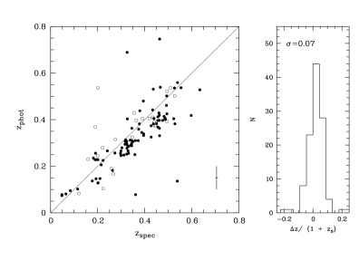
Figure 6: Left panel: photometric versus spectroscopic redshifts for the objects reported in Table 8. The black dots represent the galaxies with well determined spectroscopic redshifts, while the open circles represent the 24 galaxies with dubious redshift determinations (indicated with a “?” next to $z_{spec}$ in Table 8). The continuous line represents the relation z_phot = z_spec; right panel: distribution of the difference z_spec - z_phot.

Figure 7: Distribution of photometric redshifts of the high S/N OACDF catalog (continuous line) compared with the redshift distribution of the CFRS (dashed line) at the same depth.

Despite the dubious redshifts, the vast majority of the photometric redshifts match well the spectroscopic redshifts within the errors. Six out of 113 objects fall off the general trend (a percentage compatible with that of previous works). We find that the mean difference between photometric and spectroscopic redshifts is 0.02$\pm$0.07 (see Figure 6 right panel). Therefore, our photometric redshift determinations are confident within an RMS error of about 0.07, in the redshift range from 0 to 0.7.

The distribution of photometric redshifts of the OACDF, is shown in Figure 7. The distribution of the CFRS (Canada France Redshift Survey, Lilly et al. (1995)) is over-plotted with a dashed line for comparison.

For the sake of this comparison, we have selected two classes of objects from the whole catalog: i) the bright class is composed by objects with a high photometric S/N ratio and hence, objects for which the results obtained from the comparison with the spectroscopic follow-up are consistent; ii) the faint class, i.e. all the objects fainter than $V_{AB}=$ 22 mag. Although the latter were detected with a S/N $>$ 10, we still flagged them because we do not have any spectroscopic confirmation of their redshifts. The figure shows the objects in the bright class only.

In order to confirm the similarity of the two redshift distributions shown in Figure 7 we performed a Kolmogorov-Smirnov two sample test (KS test), which is a non-parametric test that yields correct probabilities without conditions for the distribution of the errors. The result of the KS test is that the two redshift distributions are similar at the 99.4% confidence level. We can thus conclude that the two distributions come from the same parent distribution.

6 Search for groups and clusters of galaxies

An accurate knowledge of the global properties of galaxy clusters and groups is needed both to constrain the models of galaxy formation and evolution and to falsify the cosmological models. The first step in the study of galaxy clusters is, however, the construction of statistically significant and unbiased catalogues of cosmic structures spanning a wide range of richness (N): from very low multiplicity structures such as galaxy triplets (N=3), to groups (N$<$50), and clusters (N$>$50). While much work has been devoted to the construction of complete rich cluster samples, the low multiplicity end of the structure spectrum is still poorly known due to the difficulties encountered in identifying physically bound systems of low multiplicity on wide field or survey material. On projected data, in fact, loose and poor groups of galaxies produce low signal/noise overdensities which are difficult to detect on shallow photometric material and require spectroscopic surveys and/or deep fields covering moderately wide areas.

Not so much work has been done to detect poor structures such as loose groups; two principal methods (and their successive elaborations) have been adopted. In particular, Turner & Gott (1976) presented the first tentative objective identification of groups as enhancements above a reliable threshold in the projected galaxy distribution. A noticeable exception to the lack of low-richness catalogs has been the detection of compact groups, where several teams (de Carvalho & Djorgovski 1995; Iovino et al. 1999, 2003) have proposed different approaches to their detection. For the determination of the mass function, it is important to note that its derivation from the above-cited catalogues is hindered by the fact that all of the above algorithms are optimized for the detection of either groups or clusters, and with a few exceptions (cf. Puddu et al. 2003) no systematic work has been done in matching their outcomes in the transition region between structures of low and high richness. The OACDF, as any other deep field, offers the possibility to begin covering this gap. In fact, by assuming an Euclidean metric and uniform distribution we expect to find in the OACDF ca. 5 groups in the richness range [5,30] (against less than one rich cluster). Since the investigated area of the OACDF is limited to 0.5 $\deg^{2}$, we expect to find about 4 groups in the richness range [5,30] and less than one cluster in the richness range [30,100], in the volume enclosed within 0.5 $\deg^{2}$ and z$<$1.0.

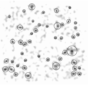
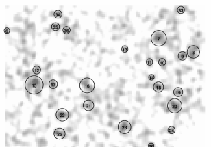
Figure 8: Smoothed density maps of the OACDF2 (top) and OACDF4 (bottom) fields. Each map has been produced by binning the matched catalogs (in the $B$, $V$ and $R$ bands) into equal area square bins of $18\times 18$ squared arc-sec (see Puddu et al. 2003 for details). The circles mark the detected over-densities (including those having a low S/N ratio).

In order to actually detect them we used the method developed by Puddu et al. (2003) and already applied to the DPOSS data (about 300 $\deg^{2}$; see Puddu et al. 2001). In summary: we first extracted a catalogue containing all extended sources with 20.5 $<R<$ 24 and then binned the corresponding galaxy spatial distribution into equal area square bins to produce a density map, such that the mean number of galaxies per bin is $\sim 1$ (binsize=0.005 deg). In order to identify and extract the density peaks on the resulting density map, we run SExtractor (after background independent estimation and subtraction) with an absolute threshold of 0.5 (objects/pixel) and a minimum detection area of 4 pixels. The background subtraction removes all the structures with spatial frequencies smaller than the scale length of 50 pixels, which corresponds to linear dimensions of $3-4$ Mpc, in the redshift range $0.3,0.6$. For the background galaxies, we find a mean density of $\sim 43000\pm 4200$ objects per square degree. In order to enhance the structures, the detection was ran on the density map convolved with a Gaussian filter $3$ pixels wide (corresponding to 150-250 kpc, at redshift $0.3-1.0$). The latter are reliable dimensions for a cluster core. A caveat of our method is that the Gaussian filter sets strong limitations on the possibility of detecting structures at higher redshifts, which appear with a more compact core than the minimum dimension of the filter itself. The over-density regions are defined by the isodensity contours corresponding to the detection threshold on a smoothed map (Figure 8). The area defined by these contours is called the iso-area. We used the number of objects lying inside this area to give an estimate of the cluster candidate richness. The error on the richness estimate depends on the S/N ratio of the detection and is inversely correlated with the richness itself: low and intermediate richness ($<$ 30) candidates have a low detection S/N and hence are not detected with an high confidence. We then use colour-magnitude diagrams to look for a possible red sequence of early type galaxies, confirming that the overdensity corresponds to a galaxy cluster.

The cluster red sequence can be isolated from the background objects using a pair of filters, if these filters sample the 4000Å break. In our case we chose the $(V-R_{C})$ color and, in order to explore a larger redshift range, we also use the $V-913$ color. There is, however, the caveat that the limiting magnitude in the narrow band filters is brighter than for the $V$ and $R_{C}$ bands with the consequence that not all the objects present in the $(V-R_{C})$ sample will be retrieved in the $V-913$ sample. However, this is not a problem for our analysis because we are interested in the bright ellipticals of the red sequence rather than in faint background galaxies.

For each over-density, we plot the color-magnitude diagrams $(V-R_{C})$ vs. $R_{C}$ and $V-913$ vs. 913 of all the objects in an aperture with an area equivalent to three times the iso-area and centered on the over-density centroid. We then select a comparison field in an annular region centered on the cluster, with a much larger radius, but with comparable area as that defined by the over-density. We then perform a statistical subtraction of the background contribution, which consists on the elimination of the points nearest to the neighbor background points in the color-magnitude diagram. In this way, the red sequence is enhanced, if it is really present. As an example, we show in Figure 9 the procedure applied to the cluster candidate OACDF-CLG02.

Figure 9: Example of the statistical subtraction applied to the cluster candidate OACDF2_2. The $(V-R_{C})$ vs. $R_{C}$ diagram for all the objects (cluster plus background) in the over-density region is shown in the upper panel, while the same diagram for the background objects is shown in the middle panel; the results after the statistical subtraction are shown in the bottom panel.

Table 5: Candidates for clusters of galaxies

candidate	RA(2000)	DEC (2000)	richness	iso-area	S/N	ph_z
				(pixs)
OACDF-CLG01	12  23  58	-12  44  53	59	30	5.7	0.3
OACDF-CLG02∗	12  24  47	-12  48  56	49	20	5.3	0.2
OACDF-CLG03	12  23  56	-12  27  29	36	26	4.3	0.5
OACDF-CLG04	12  25  00	-12  34  32	22	12	3.4	0.3
OACDF-CLG05	12  25  27	-12  46  14	25	17	3.7	0.3
OACDF-CLG06	12  23  32	-12  53  20	32	23	4.1	0.3
OACDF-CLG07	12  25  04	-13  01  41	65	32	6.1	0.2
OACDF-CLG08	12  24  25	-13  01  47	28	21	3.9	0.3
OACDF-CLG09	12  23  18	-13  02  58	17	8	3.3	0.1
OACDF-CLG10	12  23  21	-13  05  27	46	20	5.2	0.2
*: This cluster has been spectroscopically confirmed.

Ten candidates for clusters of galaxies were selected. However, we note that a large number of low S/N over-densities, that coincide with many groups of galaxies, is detected in the OACDF. In Figure 10 we plot the $(V-R_{C})$ vs. $R_{C}$ and $V-913$ vs. 913 color-magnitude diagrams of our four best cases selected on the OACDF2 and OACDF4 after the statistical subtraction of the background objects on the color-magnitude plane.

The coordinates, estimated richness, iso-area (in pixels), S/N ratio and the estimated photometric redshift for a list of galaxy cluster candidates, detected with S/N$>$3 and selected on the basis of their red sequences, is provided in Table 5. The coordinates correspond to the over-density centroids. The richness estimate was done as described above. The photometric redshift for each candidate was estimated as the median of the photometric redshifts of the objects in the corresponding aperture (three times the iso-area).

It is interesting to note that the color-magnitude diagram of the cluster candidate OACDF-CLG02 shows some hint of a double red sequence, which is more evident in the $V-913$ vs. 913 diagram. This leads to the idea of two galaxy clusters at different redshifts (one at z=0.23 and the other one at z$\approx$0.6) which by chance projection fall approximately along the same line of sight. The spectroscopic observations reported in Section 5 confirm the first galaxy cluster at z=0.20. This cluster is also known as LCDCS 0522, and was first discovered in the Las Campanas Distant Cluster Survey (Gonzalez et al. 2001), which estimated the redshift to be $z\simeq 0.34$. Given the uncertainty of about 0.1 in the latter redshift, and considering that the redshift of this cluster was confirmed spectroscopically by us using spectra of seven galaxies in the cluster, we take as correct our redshift determination.

Figure 10: Color – magnitude diagrams of our four best candidates, after applying the statistical subtraction of the background objects. The ”$\times$” symbol on the (V-R_C) vs. R_C diagrams represents the color corresponding to the photometric redshift reported in Table 5.

7 Summary

The OACDF, which comprises a photometric and astrometric database for galactic and extragalactic research, has been presented. The observations (imaging and spectroscopy), data reduction and photometric calibration, as well as the source extraction techniques, were descrived.

During the course of the observations with the WFI at the ESO 2.2m telescope, a photometric inhomogeneity was found that may be attributed, at least in part, to an additional-light pattern due to internal reflections off the telescope corrector, that may yield photometric errors of up to 3% in the $B$, $V$, $R$ and $I$ broad-bands and up to 5% in the medium-band filters.

The quality assessment studies of the OACDF provide the following results: the galaxy number counts of the OACDF deep data, in the $B$, $V$ and $R$ bands, are consistent with those from the literature; the resulting photometric redshifts, for objects brighter than about $V=$23, are consistent with the spectroscopic redshifts within a RMS error of about 0.07 in the redshift range from 0 to 0.7; the distribution of photometric redshifts of OACDF sources is consistent with that of the CFRS at the 99.4% confidence level. The relationship between observed stellar colors and stellar spectral types for the 59 stars in our spectroscopic sample fits well the intrinsic color versus spectral type relation in the spectral range from A5 to M5. This confirms the low interstellar extinction of these stars, and hence the low galactic extinction in the OACDF.

We therefore conclude that the depth of the OACDF and its relatively large spatial coverage with respect to pencil beam surveys make it a good tool for extragalactic and stellar studies. In particular it is well suited for the definition of a statistically significant sample of early type galaxies for subsequent studies of galaxy formation and evolution in the redshift range 0–1.

The OACDF also comprises a suitable database for the search for groups of galaxies and intermediate richness ($N_{gal}<100$) clusters at intermediate redshift. Applying our cluster detection algorithms, several candidates for clusters of galaxies were detected above the 3$\sigma$ level. Using the criterion of the red sequence in the color-magnitude diagram, we selected 10 candidates with estimated richness in the range from 20 to 60 and a photometric redshift in the range from 0.2 to 0.5. One of these (OACDF-CLG02) has been spectroscopically confirmed to have a redshift of 0.2. The other 9 need spectroscopic confirmation. Future studies of these cluster candidates will allow us to improve our knowledge of the different evolutionary histories of galaxies in different enviroments. The multiband and sky coverage of the OACDF make it a suitable survey to test the predictions of different theoretical scenarios at intermediate and high redshift.

Appendix A The Catalog

In this appendix we provide a catalog containing magnitudes and spectroscopic information for the 173 objects. The catalog is given in Tables 6, 7 and 8.

The broad-band AB magnitudes reported in the catalog can be transformed into the Johnson-Cousins system by applying the following expressions:

$$V=0.870\cdot V_{AB}+0.130\cdot R_{AB}-0.030$$ (9)

$$R_{C}=1.030\cdot R_{AB}-0.030\cdot V_{AB}-0.221$$ (10)

$$I_{C}=0.907\cdot I_{AB}+0.093\cdot V_{AB}-0.462$$ (11)

$$B=1.311\cdot B_{AB}-0.311\cdot V+0.122$$ (12)

Table 6: Coordinates and broad-band AB magnitudes for 173 objects in the OACDF2

OACDF	RA(2000)	DEC(2000)	$B_{AB}$	$V_{AB}$	$R_{AB}$	$I_{AB}$
122325.1-123757	12:23:25.077	-12:37:57.33	22.72$\pm$0.07	22.11$\pm$0.05	20.97$\pm$0.03	19.95$\pm$0.10
122325.4-123915	12:23:25.418	-12:39:15.02	19.98$\pm$0.04	19.05$\pm$0.03	18.24$\pm$0.03	17.06$\pm$0.08
122327.4-123714	12:23:27.351	-12:37:13.67	22.00$\pm$0.05	21.38$\pm$0.03	20.69$\pm$0.03	19.94$\pm$0.10
122327.5-123718	12:23:27.464	-12:37:18.25	21.86$\pm$0.05	21.08$\pm$0.03	20.07$\pm$0.03	19.22$\pm$0.09
122328.0-123711	12:23:28.041	-12:37:10.83	23.14$\pm$0.06	22.31$\pm$0.04	21.13$\pm$0.03	20.27$\pm$0.10
122328.2-123830	12:23:28.191	-12:38:29.94	21.20$\pm$0.04	20.13$\pm$0.03	19.48$\pm$0.03	18.80$\pm$0.08
122328.8-123610	12:23:28.810	-12:36:09.52	23.36$\pm$0.08	22.56$\pm$0.05	21.74$\pm$0.03	20.25$\pm$0.09
122329.0-123839	12:23:29.022	-12:38:39.18	21.26$\pm$0.04	20.59$\pm$0.03	20.15$\pm$0.03	19.80$\pm$0.09
122329.7-123827	12:23:29.707	-12:38:26.65	21.10$\pm$0.04	20.23$\pm$0.03	19.69$\pm$0.03	18.91$\pm$0.08
122330.6-123857	12:23:30.604	-12:38:56.89	22.31$\pm$0.04	20.71$\pm$0.03	19.62$\pm$0.03	18.66$\pm$0.08
122330.7-123740	12:23:30.656	-12:37:40.28	20.71$\pm$0.04	20.63$\pm$0.03	19.62$\pm$0.03	18.94$\pm$0.09
122331.7-123945	12:23:31.705	-12:39:45.03	18.27$\pm$0.04	17.70$\pm$0.03	17.25$\pm$0.03	16.84$\pm$0.08
122332.5-123720	12:23:32.499	-12:37:20.10	22.23$\pm$0.05	21.24$\pm$0.03	20.32$\pm$0.03	19.50$\pm$0.09
122332.7-123940	12:23:32.652	-12:39:40.47	22.74$\pm$0.05	21.86$\pm$0.04	20.85$\pm$0.03	19.84$\pm$0.09
122333.7-123715	12:23:33.665	-12:37:15.42	21.57$\pm$0.05	20.77$\pm$0.03	19.66$\pm$0.03	19.06$\pm$0.09
122336.0-123907	12:23:35.992	-12:39:07.06	21.18$\pm$0.04	20.23$\pm$0.03	19.28$\pm$0.03	18.60$\pm$0.08
122336.1-123811	12:23:36.126	-12:38:11.03	21.80$\pm$0.04	21.23$\pm$0.03	20.57$\pm$0.03	19.93$\pm$0.09
122336.2-123652	12:23:36.158	-12:36:51.75	21.97$\pm$0.05	21.37$\pm$0.04	20.94$\pm$0.03	20.49$\pm$0.13
122337.4-123813	12:23:37.425	-12:38:12.79	22.31$\pm$0.06	21.38$\pm$0.04	20.65$\pm$0.03	19.70$\pm$0.10
122338.5-123829	12:23:38.540	-12:38:29.47	20.57$\pm$0.04	19.61$\pm$0.03	19.08$\pm$0.03	18.58$\pm$0.08
122339.4-123829	12:23:39.413	-12:38:29.25	21.90$\pm$0.05	21.12$\pm$0.03	20.69$\pm$0.03	20.04$\pm$0.10
122339.7-123928	12:23:39.656	-12:39:28.49	22.74$\pm$0.06	21.82$\pm$0.04	21.13$\pm$0.03	20.50$\pm$0.10
122340.6-123830	12:23:40.562	-12:38:30.22	21.91$\pm$0.04	21.24$\pm$0.03	20.98$\pm$0.03	20.33$\pm$0.10
122340.8-123752	12:23:40.815	-12:37:52.40	22.67$\pm$0.06	22.13$\pm$0.04	20.87$\pm$0.03	20.46$\pm$0.10
122341.1-124121	12:23:41.114	-12:41:20.65	21.93$\pm$0.05	21.32$\pm$0.03	20.59$\pm$0.03	19.69$\pm$0.10
122341.4-124032	12:23:41.357	-12:40:31.64	22.45$\pm$0.05	21.45$\pm$0.03	20.58$\pm$0.03	18.99$\pm$0.08
122341.8-123860	12:23:41.752	-12:38:59.99	22.51$\pm$0.06	21.55$\pm$0.04	20.43$\pm$0.03	19.48$\pm$0.09
122342.2-123904	12:23:42.231	-12:39:03.92	22.35$\pm$0.05	21.71$\pm$0.03	21.44$\pm$0.03	21.09$\pm$0.12
122343.0-123704	12:23:42.950	-12:37:04.20	15.53$\pm$0.04	15.20$\pm$0.03	15.35$\pm$0.03	14.69$\pm$0.08
122343.2-123919	12:23:43.183	-12:39:19.11	22.64$\pm$0.05	22.16$\pm$0.04	21.59$\pm$0.03	20.96$\pm$0.13
122343.4-123756	12:23:43.406	-12:37:56.02	19.56$\pm$0.04	18.70$\pm$0.03	17.97$\pm$0.03	17.10$\pm$0.08
122344.2-123700	12:23:44.157	-12:37:00.00	22.17$\pm$0.05	21.04$\pm$0.03	20.17$\pm$0.03	19.35$\pm$0.08
122344.3-123816	12:23:44.276	-12:38:15.67	20.73$\pm$0.04	20.51$\pm$0.03	20.41$\pm$0.03	20.26$\pm$0.09
122344.6-123908	12:23:44.565	-12:39:08.43	21.75$\pm$0.05	21.17$\pm$0.04	20.28$\pm$0.03	19.64$\pm$0.10
122345.1-123748	12:23:45.100	-12:37:48.26	22.65$\pm$0.05	22.02$\pm$0.04	21.71$\pm$0.03	21.15$\pm$0.12
122346.2-123933	12:23:46.150	-12:39:32.67	22.27$\pm$0.05	21.34$\pm$0.03	20.71$\pm$0.03	20.00$\pm$0.09
122347.0-123937	12:23:47.039	-12:39:36.56	22.02$\pm$0.05	21.03$\pm$0.03	20.13$\pm$0.03	19.35$\pm$0.09
122347.5-123759	12:23:47.515	-12:37:59.31	21.73$\pm$0.05	20.96$\pm$0.03	20.37$\pm$0.03	19.59$\pm$0.09
122348.5-123915	12:23:48.468	-12:39:15.29	18.83$\pm$0.04	18.42$\pm$0.03	18.18$\pm$0.03	17.91$\pm$0.08
122348.5-124055	12:23:48.539	-12:40:55.46	20.59$\pm$0.04	19.60$\pm$0.03	19.11$\pm$0.03	18.55$\pm$0.08
122348.7-123748	12:23:48.695	-12:37:47.74	21.87$\pm$0.04	21.14$\pm$0.03	20.48$\pm$0.03	19.84$\pm$0.09
122349.4-124121	12:23:49.369	-12:41:20.87	20.94$\pm$0.04	20.60$\pm$0.03	20.39$\pm$0.03	20.14$\pm$0.09
122349.4-124144	12:23:49.394	-12:41:44.48	22.64$\pm$0.05	21.77$\pm$0.04	20.58$\pm$0.03	19.76$\pm$0.09
122349.7-123939	12:23:49.650	-12:39:38.51	22.82$\pm$0.05	21.66$\pm$0.03	20.74$\pm$0.03	18.89$\pm$0.08
122350.0-123708	12:23:49.963	-12:37:07.91	22.84$\pm$0.05	21.82$\pm$0.04	20.97$\pm$0.03	19.62$\pm$0.08
122350.2-124223	12:23:50.230	-12:42:23.16	20.57$\pm$0.04	19.57$\pm$0.03	18.72$\pm$0.03	16.99$\pm$0.08
122351.4-124012	12:23:51.437	-12:40:12.45	22.32$\pm$0.05	21.88$\pm$0.05	21.36$\pm$0.04	20.86$\pm$0.16
122352.1-123732	12:23:52.055	-12:37:31.50	21.00$\pm$0.04	20.14$\pm$0.03	19.32$\pm$0.03	17.79$\pm$0.08
122352.4-123905	12:23:52.364	-12:39:05.49	21.58$\pm$0.04	20.88$\pm$0.03	20.59$\pm$0.03	20.17$\pm$0.11
122354.7-124112	12:23:54.719	-12:41:12.28	21.64$\pm$0.04	20.85$\pm$0.03	20.01$\pm$0.03	18.86$\pm$0.08
122355.6-123904	12:23:55.573	-12:39:04.24	21.94$\pm$0.05	20.99$\pm$0.03	20.33$\pm$0.03	19.79$\pm$0.09
122418.3-122832	12:24:18.334	-12:28:32.24	21.89$\pm$0.05	21.22$\pm$0.03	20.32$\pm$0.03	19.67$\pm$0.09
122418.9-122655	12:24:18.948	-12:26:54.93	21.39$\pm$0.04	20.39$\pm$0.03	19.47$\pm$0.03	18.66$\pm$0.08
122420.0-122935	12:24:20.024	-12:29:34.83	22.39$\pm$0.06	21.65$\pm$0.04	21.03$\pm$0.03	20.87$\pm$0.13
122421.1-122737	12:24:21.136	-12:27:36.89	21.80$\pm$0.05	20.85$\pm$0.03	19.98$\pm$0.03	19.28$\pm$0.09
122421.4-122854	12:24:21.420	-12:28:54.34	21.65$\pm$0.05	21.27$\pm$0.04	20.03$\pm$0.03	19.44$\pm$0.09
122422.1-122720	12:24:22.148	-12:27:19.71	20.60$\pm$0.04	19.95$\pm$0.03	19.64$\pm$0.03	19.31$\pm$0.09
122423.4-122901	12:24:23.380	-12:29:00.79	21.96$\pm$0.07	20.41$\pm$0.04	20.35$\pm$0.03	19.81$\pm$0.09
122424.5-122855	12:24:24.464	-12:28:54.73	20.29$\pm$0.04	20.02$\pm$0.03	19.88$\pm$0.03	20.12$\pm$0.09
122425.0-123011	12:24:24.984	-12:30:11.17	22.03$\pm$0.05	21.53$\pm$0.04	20.85$\pm$0.03	20.48$\pm$0.14

Table 5. Continued

OACDF	RA(2000)	DEC(2000)	$B_{AB}$	$V_{AB}$	$R_{AB}$	$I_{AB}$
122426.5-123002	12:24:26.499	-12:30:02.32	21.98$\pm$0.04	21.70 $\pm$0.03	21.57$\pm$0.03	21.43$\pm$0.13
122426.6-121947	12:24:26.610	-12:19:47.24	16.58$\pm$0.04	16.41 $\pm$0.03	16.60$\pm$0.03	16.64$\pm$0.08
122427.4-122313	12:24:27.382	-12:23:13.46	22.20$\pm$0.05	21.17 $\pm$0.03	20.29$\pm$0.03	18.50$\pm$0.08
122427.4-122924	12:24:27.424	-12:29:24.21	16.79$\pm$0.04	16.40 $\pm$0.03	16.26$\pm$0.03	16.06$\pm$0.08
122427.9-122720	12:24:27.886	-12:27:19.90	22.16$\pm$0.05	21.55 $\pm$0.04	20.88$\pm$0.03	20.34$\pm$0.12
122428.5-122725	12:24:28.515	-12:27:24.54	22.35$\pm$0.05	21.83 $\pm$0.04	21.19$\pm$0.03	20.61$\pm$0.13
122429.3-122021	12:24:29.313	-12:20:21.41	21.57$\pm$0.05	20.88 $\pm$0.03	20.39$\pm$0.03	19.75$\pm$0.11
122429.5-122710	12:24:29.466	-12:27:09.86	22.24$\pm$0.05	21.44 $\pm$0.03	20.61$\pm$0.03	19.80$\pm$0.09
122430.1-122822	12:24:30.089	-12:28:21.84	22.77$\pm$0.07	21.93 $\pm$0.05	20.82$\pm$0.03	20.12$\pm$0.10
122430.7-122315	12:24:30.713	-12:23:15.34	21.11$\pm$0.04	20.19 $\pm$0.03	19.42$\pm$0.03	18.53$\pm$0.08
122430.8-122913	12:24:30.762	-12:29:12.58	21.91$\pm$0.04	20.90 $\pm$0.03	20.07$\pm$0.03	18.83$\pm$0.08
122431.0-124601	12:24:30.996	-12:46:00.72	22.20$\pm$0.05	21.13 $\pm$0.03	20.27$\pm$0.03	19.57$\pm$0.09
122431.2-122113	12:24:31.206	-12:21:13.05	22.78$\pm$0.07	22.22 $\pm$0.04	21.30$\pm$0.03	20.60$\pm$0.10
122431.8-124736	12:24:31.768	-12:47:36.13	20.71$\pm$0.04	19.84 $\pm$0.03	19.37$\pm$0.03	18.83$\pm$0.08
122432.0-121914	12:24:32.016	-12:19:14.04	22.59$\pm$0.08	–	-	18.80$\pm$0.06
122432.4-124937	12:24:32.416	-12:49:36.65	22.27$\pm$0.05	21.76 $\pm$0.04	21.37$\pm$0.03	21.12$\pm$0.11
122432.7-122616	12:24:32.673	-12:26:16.24	22.68$\pm$0.05	21.92 $\pm$0.04	20.94$\pm$0.03	20.17$\pm$0.10
122432.8-121937	12:24:32.801	-12:19:36.83	18.86$\pm$0.04	18.30 $\pm$0.03	17.79$\pm$0.03	17.23$\pm$0.08
122433.6-122647	12:24:33.571	-12:26:47.35	23.37$\pm$0.07	21.98 $\pm$0.04	20.78$\pm$0.03	19.65$\pm$0.09
122434.4-124801	12:24:34.363	-12:48:01.08	19.41$\pm$0.04	19.15 $\pm$0.03	19.04$\pm$0.03	18.95$\pm$0.08
122434.5-122847	12:24:34.519	-12:28:46.86	21.62$\pm$0.04	20.71 $\pm$0.03	20.00$\pm$0.03	19.45$\pm$0.08
122434.7-122151	12:24:34.656	-12:21:51.09	22.65$\pm$0.05	21.84 $\pm$0.04	21.14$\pm$0.03	20.43$\pm$0.09
122434.8-122911	12:24:34.841	-12:29:11.07	21.06$\pm$0.04	20.31 $\pm$0.03	19.92$\pm$0.03	19.34$\pm$0.09
122435.2-124947	12:24:35.183	-12:49:46.90	21.99$\pm$0.05	21.29 $\pm$0.03	20.96$\pm$0.03	20.32$\pm$0.11
122435.4-121903	12:24:35.396	-12:19:03.48	22.57$\pm$0.07	21.74 $\pm$0.05	20.66$\pm$0.03	19.79$\pm$0.11
122435.4-122811	12:24:35.443	-12:28:11.06	23.79$\pm$0.09	22.67 $\pm$0.05	21.42$\pm$0.03	20.17$\pm$0.10
122436.1-122807	12:24:36.133	-12:28:06.84	22.63$\pm$0.05	21.62 $\pm$0.03	20.71$\pm$0.03	20.23$\pm$0.08
122436.1-124757	12:24:36.135	-12:47:57.29	21.51$\pm$0.04	21.05 $\pm$0.03	20.56$\pm$0.03	18.92$\pm$0.10
122436.7-122645	12:24:36.651	-12:26:45.18	15.55$\pm$0.04	15.20 $\pm$0.03	15.28$\pm$0.03	14.51$\pm$0.08
122436.7-124519	12:24:36.721	-12:45:18.84	22.70$\pm$0.05	21.87 $\pm$0.04	21.79$\pm$0.03	21.43$\pm$0.12
122437.4-124654	12:24:37.432	-12:46:54.25	19.09$\pm$0.04	18.14 $\pm$0.03	17.33$\pm$0.03	16.33$\pm$0.08
122437.5-122835	12:24:37.515	-12:28:35.05	22.86$\pm$0.08	22.06 $\pm$0.05	21.14$\pm$0.03	20.10$\pm$0.10
122437.7-122019	12:24:37.653	-12:20:19.28	22.80$\pm$0.07	22.01 $\pm$0.04	21.36$\pm$0.03	20.51$\pm$0.11
122438.2-122910	12:24:38.210	-12:29:09.67	22.72$\pm$0.06	21.95 $\pm$0.04	20.96$\pm$0.03	19.90$\pm$0.10
122438.5-124638	12:24:38.458	-12:46:38.49	22.68$\pm$0.05	21.55 $\pm$0.03	20.65$\pm$0.03	18.66$\pm$0.08
122438.9-122004	12:24:38.916	-12:20:04.42	22.11$\pm$0.05	21.20 $\pm$0.03	20.43$\pm$0.03	19.25$\pm$0.08
122439.1-122942	12:24:39.109	-12:29:41.80	22.71$\pm$0.05	21.62 $\pm$0.03	20.78$\pm$0.03	19.06$\pm$0.08
122439.2-124713	12:24:39.219	-12:47:13.47	22.03$\pm$0.04	21.10 $\pm$0.03	20.36$\pm$0.03	19.46$\pm$0.08
122440.0-124847	12:24:40.008	-12:48:47.10	20.37$\pm$0.04	20.04 $\pm$0.03	19.89$\pm$0.03	19.82$\pm$0.08
122440.2-122843	12:24:40.152	-12:28:42.56	19.90$\pm$0.04	19.13 $\pm$0.03	18.42$\pm$0.03	17.75$\pm$0.08
122440.8-121902	12:24:40.766	-12:19:02.10	23.73$\pm$0.10	22.58 $\pm$0.06	21.24$\pm$0.04	20.87$\pm$0.16
122440.9-124920	12:24:40.891	-12:49:19.82	20.73$\pm$0.04	20.41 $\pm$0.03	20.26$\pm$0.03	20.05$\pm$0.09
122441.5-122924	12:24:41.452	-12:29:23.73	21.75$\pm$0.05	20.83 $\pm$0.03	20.28$\pm$0.03	19.68$\pm$0.09
122442.0-122211	12:24:42.013	-12:22:10.60	18.94$\pm$0.04	18.65 $\pm$0.03	18.52$\pm$0.03	18.30$\pm$0.08
122442.1-124843	12:24:42.052	-12:48:42.71	21.04$\pm$0.04	20.12 $\pm$0.03	19.53$\pm$0.03	19.02$\pm$0.08
122442.4-122833	12:24:42.381	-12:28:32.76	21.75$\pm$0.04	21.05 $\pm$0.03	20.39$\pm$0.03	19.87$\pm$0.08
122442.9-122909	12:24:42.931	-12:29:08.51	21.88$\pm$0.04	21.41 $\pm$0.03	21.00$\pm$0.03	20.62$\pm$0.10
122442.9-124841	12:24:42.947	-12:48:41.05	20.26$\pm$0.04	19.39 $\pm$0.03	18.78$\pm$0.03	18.22$\pm$0.08
122443.3-124626	12:24:43.327	-12:46:26.21	23.44$\pm$0.10	22.22 $\pm$0.05	20.99$\pm$0.03	19.85$\pm$0.09
122443.5-121838	12:24:43.466	-12:18:37.67	19.38$\pm$0.04	18.75 $\pm$0.03	18.42$\pm$0.03	17.97$\pm$0.08
122443.7-122610	12:24:43.687	-12:26:09.90	21.23$\pm$0.04	20.69 $\pm$0.03	20.43$\pm$0.03	20.07$\pm$0.10
122444.0-124810	12:24:44.010	-12:48:09.83	22.16$\pm$0.05	21.18 $\pm$0.03	20.68$\pm$0.03	20.13$\pm$0.10
122444.2-122138	12:24:44.190	-12:21:38.02	22.45$\pm$0.05	21.86 $\pm$0.04	21.15$\pm$0.03	20.41$\pm$0.10
122444.6-122907	12:24:44.554	-12:29:07.33	17.22$\pm$0.04	17.04 $\pm$0.03	16.93$\pm$0.03	16.82$\pm$0.08
122445.2-122916	12:24:45.236	-12:29:16.38	18.17$\pm$0.04	17.76 $\pm$0.03	17.51$\pm$0.03	17.23$\pm$0.08
122445.7-122243	12:24:45.679	-12:22:42.56	22.61$\pm$0.07	21.75 $\pm$0.04	20.61$\pm$0.03	19.55$\pm$0.09
122445.8-124838	12:24:45.780	-12:48:37.68	20.56$\pm$0.04	19.66 $\pm$0.03	19.13$\pm$0.03	18.61$\pm$0.08
122446.6-122151	12:24:46.611	-12:21:50.88	22.34$\pm$0.07	21.57 $\pm$0.04	20.32$\pm$0.03	19.23$\pm$0.09
122447.5-122736	12:24:47.532	-12:27:36.11	21.44$\pm$0.04	20.55 $\pm$0.03	19.72$\pm$0.03	18.53$\pm$0.08
122447.6-121845	12:24:47.554	-12:18:44.66	19.46$\pm$0.04	19.11 $\pm$0.03	18.98$\pm$0.03	18.70$\pm$0.09

Table 5. Continued

OACDF	RA(2000)	DEC(2000)	$B_{AB}$	$V_{AB}$	$R_{AB}$	$I_{AB}$
122447.6-124852	12:24:47.640	-12:48:52.32	23.21$\pm$0.10	22.22$\pm$0.06	20.91$\pm$0.03	20.05$\pm$0.09
122448.2-122137	12:24:48.170	-12:21:37.21	23.61$\pm$0.10	23.02$\pm$0.06	22.20$\pm$0.04	21.43$\pm$0.13
122448.5-122847	12:24:48.505	-12:28:47.13	22.16$\pm$0.05	21.08$\pm$0.03	20.13$\pm$0.03	19.45$\pm$0.09
122448.8-124703	12:24:48.842	-12:47:02.94	21.52$\pm$0.04	20.84$\pm$0.03	20.52$\pm$0.03	19.97$\pm$0.10
122448.9-122153	12:24:48.916	-12:21:53.27	22.73$\pm$0.06	21.86$\pm$0.04	21.12$\pm$0.03	20.28$\pm$0.10
122449.4-124851	12:24:49.404	-12:48:50.84	19.73$\pm$0.04	18.81$\pm$0.03	18.23$\pm$0.03	17.71$\pm$0.08
122450.6-124550	12:24:50.615	-12:45:50.09	21.05$\pm$0.04	20.84$\pm$0.03	20.75$\pm$0.03	20.62$\pm$0.10
122451.2-122013	12:24:51.227	-12:20:13.06	14.96$\pm$0.04	14.83$\pm$0.03	14.96$\pm$0.03	14.20$\pm$0.08
122451.3-124722	12:24:51.336	-12:47:21.93	21.84$\pm$0.04	21.52$\pm$0.03	21.21$\pm$0.03	21.15$\pm$0.11
122452.0-122230	12:24:52.033	-12:22:29.75	22.01$\pm$0.05	21.15$\pm$0.03	20.33$\pm$0.03	19.52$\pm$0.09
122452.3-124827	12:24:52.307	-12:48:27.24	21.83$\pm$0.05	21.29$\pm$0.03	21.12$\pm$0.03	20.91$\pm$0.14
122453.1-122249	12:24:53.062	-12:22:49.26	21.76$\pm$0.05	20.92$\pm$0.03	19.94$\pm$0.03	19.24$\pm$0.08
122453.4-124520	12:24:53.368	-12:45:20.24	21.78$\pm$0.04	20.75$\pm$0.03	19.97$\pm$0.03	19.40$\pm$0.08
122453.5-122059	12:24:53.491	-12:20:59.41	21.34$\pm$0.04	20.87$\pm$0.03	20.07$\pm$0.03	19.60$\pm$0.09
122454.3-124536	12:24:54.322	-12:45:35.89	21.83$\pm$0.04	21.03$\pm$0.03	20.55$\pm$0.03	19.99$\pm$0.10
122454.3-122124	12:24:54.333	-12:21:24.45	19.01$\pm$0.04	18.56$\pm$0.03	18.22$\pm$0.03	17.82$\pm$0.08
122455.1-122216	12:24:55.077	-12:22:15.84	22.57$\pm$0.06	21.99$\pm$0.04	20.90$\pm$0.03	19.92$\pm$0.10
122455.6-122058	12:24:55.637	-12:20:58.23	20.85$\pm$0.04	20.60$\pm$0.03	20.07$\pm$0.03	19.66$\pm$0.09
122455.6-124554	12:24:55.641	-12:45:53.98	20.94$\pm$0.04	20.17$\pm$0.03	19.51$\pm$0.03	18.74$\pm$0.08
122456.6-122206	12:24:56.611	-12:22:05.92	22.28$\pm$0.05	21.59$\pm$0.04	20.79$\pm$0.03	20.21$\pm$0.11
122457.2-124937	12:24:57.155	-12:49:36.55	21.30$\pm$0.04	20.24$\pm$0.03	19.59$\pm$0.03	18.98$\pm$0.08
122458.0-124550	12:24:57.998	-12:45:49.64	22.49$\pm$0.05	21.65$\pm$0.04	21.16$\pm$0.03	20.57$\pm$0.10
122459.0-124648	12:24:59.022	-12:46:47.88	21.27$\pm$0.04	20.34$\pm$0.03	19.53$\pm$0.03	18.58$\pm$0.08
122460.0-124616	12:24:59.979	-12:46:15.70	21.12$\pm$0.04	20.17$\pm$0.03	19.28$\pm$0.03	17.54$\pm$0.08
122500.8-124614	12:25:00.804	-12:46:13.86	19.57$\pm$0.04	19.34$\pm$0.03	19.16$\pm$0.03	19.04$\pm$0.08
122501.3-122314	12:25:01.273	-12:23:13.59	21.74$\pm$0.04	21.53$\pm$0.03	21.40$\pm$0.03	21.17$\pm$0.13
122501.5-124540	12:25:01.464	-12:45:39.78	20.08$\pm$0.04	19.63$\pm$0.03	19.34$\pm$0.03	18.97$\pm$0.08
122502.2-124853	12:25:02.173	-12:48:52.61	20.33$\pm$0.04	19.40$\pm$0.03	18.57$\pm$0.03	17.29$\pm$0.08
122502.6-122322	12:25:02.591	-12:23:21.53	18.26$\pm$0.04	17.80$\pm$0.03	17.43$\pm$0.03	17.02$\pm$0.08
122507.2-122149	12:25:07.233	-12:21:48.63	21.45$\pm$0.04	20.89$\pm$0.03	20.08$\pm$0.03	19.43$\pm$0.09
122507.5-122405	12:25:07.510	-12:24:04.90	21.75$\pm$0.05	20.78$\pm$0.03	20.03$\pm$0.03	19.40$\pm$0.09
122508.3-122216	12:25:08.294	-12:22:16.35	18.07$\pm$0.04	17.81$\pm$0.03	17.53$\pm$0.03	17.27$\pm$0.08
122508.8-122237	12:25:08.841	-12:22:36.69	17.16$\pm$0.04	16.90$\pm$0.03	16.69$\pm$0.03	16.42$\pm$0.08
122509.4-122439	12:25:09.359	-12:24:38.63	21.63$\pm$0.05	20.67$\pm$0.03	19.77$\pm$0.03	19.01$\pm$0.08
122512.1-122225	12:25:12.055	-12:22:25.16	22.52$\pm$0.05	21.72$\pm$0.03	21.00$\pm$0.03	19.63$\pm$0.08
122512.4-122424	12:25:12.362	-12:24:24.47	21.18$\pm$0.04	20.67$\pm$0.03	20.27$\pm$0.03	19.91$\pm$0.09
122512.6-122535	12:25:12.631	-12:25:34.78	22.68$\pm$0.05	22.01$\pm$0.04	21.06$\pm$0.03	20.34$\pm$0.10
122514.4-122404	12:25:14.400	-12:24:04.43	21.93$\pm$0.04	21.46$\pm$0.03	20.91$\pm$0.03	20.24$\pm$0.10
122514.7-122158	12:25:14.673	-12:21:57.97	22.81$\pm$0.07	21.59$\pm$0.05	20.38$\pm$0.03	19.60$\pm$0.09
122515.9-122624	12:25:15.932	-12:26:23.61	21.68$\pm$0.05	20.69$\pm$0.03	19.79$\pm$0.03	19.07$\pm$0.08
122516.8-122434	12:25:16.845	-12:24:33.93	21.99$\pm$0.05	21.25$\pm$0.04	20.33$\pm$0.03	19.56$\pm$0.09
122517.5-122629	12:25:17.547	-12:26:28.90	22.15$\pm$0.06	21.18$\pm$0.04	20.35$\pm$0.03	19.46$\pm$0.09
122517.7-122446	12:25:17.729	-12:24:45.88	22.43$\pm$0.06	21.81$\pm$0.04	21.20$\pm$0.03	20.59$\pm$0.13
122518.0-122448	12:25:17.993	-12:24:48.20	18.53$\pm$0.04	18.13$\pm$0.03	17.90$\pm$0.03	17.69$\pm$0.08
122519.2-122223	12:25:19.232	-12:22:23.49	20.15$\pm$0.04	19.94$\pm$0.03	19.86$\pm$0.03	19.69$\pm$0.08
122519.4-122616	12:25:19.410	-12:26:16.35	23.03$\pm$0.06	22.01$\pm$0.04	20.80$\pm$0.03	19.95$\pm$0.09
122524.6-122641	12:25:24.603	-12:26:40.60	16.55$\pm$0.04	16.24$\pm$0.03	16.10$\pm$0.03	15.92$\pm$0.08
122527.6-122328	12:25:27.559	-12:23:28.30	22.64$\pm$0.06	21.74$\pm$0.04	21.04$\pm$0.03	20.08$\pm$0.09
122528.4-122427	12:25:28.353	-12:24:26.94	21.93$\pm$0.06	21.16$\pm$0.03	20.23$\pm$0.03	19.50$\pm$0.09
122531.2-122503	12:25:31.225	-12:25:03.21	20.94$\pm$0.04	20.16$\pm$0.03	19.65$\pm$0.03	19.29$\pm$0.08
122532.3-122415	12:25:32.342	-12:24:14.79	21.96$\pm$0.05	20.93$\pm$0.03	20.09$\pm$0.03	18.38$\pm$0.08
122533.2-122457	12:25:33.181	-12:24:57.13	15.79$\pm$0.04	15.49$\pm$0.03	15.42$\pm$0.03	15.11$\pm$0.08
122534.5-122356	12:25:34.501	-12:23:55.98	22.32$\pm$0.08	21.26$\pm$0.04	20.31$\pm$0.03	19.49$\pm$0.09

Table 7: Intermediate-band AB magnitudes for 173 objects in the OACDF2

OACDF	M753	M770	M791	M816	M837	M884	M913
122325.1-123757	20.55$\pm$0.07	20.55$\pm$0.07	20.30$\pm$0.07	20.17$\pm$0.06	20.09$\pm$0.07	20.04$\pm$0.07	20.19$\pm$0.07
122325.4-123915	17.31$\pm$0.06	17.37$\pm$0.06	17.15$\pm$0.06	17.02$\pm$0.06	16.99$\pm$0.06	16.93$\pm$0.06	17.00$\pm$0.06
122327.4-123714	20.32$\pm$0.06	20.29$\pm$0.06	20.10$\pm$0.07	20.02$\pm$0.06	20.07$\pm$0.07	19.94$\pm$0.06	20.06$\pm$0.07
122327.5-123718	19.63$\pm$0.06	19.52$\pm$0.06	19.41$\pm$0.06	19.27$\pm$0.06	19.21$\pm$0.06	19.17$\pm$0.06	19.24$\pm$0.06
122328.0-123711	20.60$\pm$0.06	20.57$\pm$0.06	20.51$\pm$0.07	20.28$\pm$0.06	20.21$\pm$0.07	20.15$\pm$0.07	20.22$\pm$0.06
122328.2-123830	19.07$\pm$0.06	19.05$\pm$0.06	18.86$\pm$0.06	18.79$\pm$0.06	18.71$\pm$0.06	18.74$\pm$0.06	18.74$\pm$0.06
122328.8-123610	20.57$\pm$0.06	20.67$\pm$0.06	20.43$\pm$0.07	20.23$\pm$0.06	20.20$\pm$0.07	20.10$\pm$0.06	20.18$\pm$0.06
122329.0-123839	19.91$\pm$0.06	19.91$\pm$0.06	19.72$\pm$0.06	19.73$\pm$0.06	19.57$\pm$0.07	19.41$\pm$0.06	19.78$\pm$0.06
122329.7-123827	19.23$\pm$0.06	19.22$\pm$0.06	19.03$\pm$0.06	18.86$\pm$0.06	18.88$\pm$0.06	18.85$\pm$0.06	18.88$\pm$0.06
122330.6-123857	18.96$\pm$0.06	19.01$\pm$0.06	18.59$\pm$0.06	18.58$\pm$0.06	18.54$\pm$0.06	18.45$\pm$0.06	18.54$\pm$0.06
122330.7-123740	19.26$\pm$0.06	19.25$\pm$0.06	19.18$\pm$0.06	19.02$\pm$0.06	19.00$\pm$0.06	18.94$\pm$0.06	19.04$\pm$0.06
122331.7-123945	16.90$\pm$0.06	16.90$\pm$0.06	16.78$\pm$0.06	16.75$\pm$0.06	16.71$\pm$0.06	16.73$\pm$0.06	16.86$\pm$0.06
122332.5-123720	19.86$\pm$0.06	19.84$\pm$0.06	19.72$\pm$0.07	19.59$\pm$0.06	19.45$\pm$0.07	19.46$\pm$0.06	19.62$\pm$0.06
122332.7-123940	20.28$\pm$0.06	20.25$\pm$0.06	20.05$\pm$0.07	19.99$\pm$0.06	19.92$\pm$0.07	19.72$\pm$0.06	19.80$\pm$0.06
122333.7-123715	19.53$\pm$0.06	19.43$\pm$0.06	18.97$\pm$0.06	19.24$\pm$0.06	19.03$\pm$0.06	19.01$\pm$0.06	19.21$\pm$0.06
122336.0-123907	18.81$\pm$0.06	18.82$\pm$0.06	18.60$\pm$0.06	18.52$\pm$0.06	18.52$\pm$0.06	18.42$\pm$0.06	18.54$\pm$0.06
122336.1-123811	20.24$\pm$0.06	20.14$\pm$0.06	20.07$\pm$0.07	19.93$\pm$0.06	19.95$\pm$0.07	19.69$\pm$0.06	20.01$\pm$0.06
122336.2-123652	20.84$\pm$0.07	20.80$\pm$0.08	20.79$\pm$0.09	20.63$\pm$0.07	20.83$\pm$0.10	20.43$\pm$0.08	20.74$\pm$0.08
122337.4-123813	20.26$\pm$0.06	20.20$\pm$0.06	20.08$\pm$0.07	19.98$\pm$0.06	19.97$\pm$0.08	19.86$\pm$0.07	20.05$\pm$0.06
122338.5-123829	18.73$\pm$0.06	18.75$\pm$0.06	18.59$\pm$0.06	18.46$\pm$0.06	18.40$\pm$0.06	18.39$\pm$0.06	18.48$\pm$0.06
122339.4-123829	20.35$\pm$0.06	20.38$\pm$0.06	20.35$\pm$0.07	20.13$\pm$0.06	20.16$\pm$0.07	19.89$\pm$0.06	20.23$\pm$0.07
122339.7-123928	20.67$\pm$0.07	20.69$\pm$0.07	20.50$\pm$0.07	20.49$\pm$0.06	20.50$\pm$0.07	20.47$\pm$0.07	20.52$\pm$0.07
122340.6-123830	20.61$\pm$0.07	20.69$\pm$0.07	20.62$\pm$0.07	20.41$\pm$0.06	20.09$\pm$0.07	20.34$\pm$0.07	20.48$\pm$0.07
122340.8-123752	20.75$\pm$0.07	20.63$\pm$0.07	20.40$\pm$0.08	20.40$\pm$0.06	20.39$\pm$0.08	20.06$\pm$0.07	20.22$\pm$0.07
122341.1-124121	20.22$\pm$0.06	20.18$\pm$0.06	20.07$\pm$0.07	19.91$\pm$0.06	19.89$\pm$0.07	19.86$\pm$0.06	19.96$\pm$0.06
122341.4-124032	19.31$\pm$0.06	19.47$\pm$0.06	19.20$\pm$0.06	18.91$\pm$0.06	18.89$\pm$0.06	18.81$\pm$0.06	18.81$\pm$0.06
122341.8-123860	20.00$\pm$0.06	19.95$\pm$0.06	19.76$\pm$0.07	19.60$\pm$0.06	19.45$\pm$0.07	19.40$\pm$0.06	19.63$\pm$0.06
122342.2-123904	21.16$\pm$0.08	21.29$\pm$0.07	21.34$\pm$0.11	20.98$\pm$0.07	20.64$\pm$0.08	20.94$\pm$0.08	21.17$\pm$0.08
122343.0-123704	14.71$\pm$0.06	14.74$\pm$0.06	14.58$\pm$0.06	14.57$\pm$0.06	14.57$\pm$0.06	14.64$\pm$0.06	14.79$\pm$0.06
122343.2-123919	21.24$\pm$0.07	21.23$\pm$0.07	21.10$\pm$0.08	21.04$\pm$0.07	20.97$\pm$0.08	20.82$\pm$0.08	21.23$\pm$0.08
122343.4-123756	17.29$\pm$0.06	17.34$\pm$0.06	17.11$\pm$0.06	17.03$\pm$0.06	17.01$\pm$0.06	17.01$\pm$0.06	17.10$\pm$0.06
122344.2-123700	19.60$\pm$0.06	19.61$\pm$0.06	19.44$\pm$0.06	19.32$\pm$0.06	19.36$\pm$0.06	19.23$\pm$0.06	19.29$\pm$0.06
122344.3-123816	20.26$\pm$0.06	20.29$\pm$0.06	20.20$\pm$0.07	20.16$\pm$0.06	20.12$\pm$0.07	20.20$\pm$0.06	20.33$\pm$0.06
122344.6-123908	19.98$\pm$0.06	19.80$\pm$0.06	19.82$\pm$0.07	19.56$\pm$0.06	19.59$\pm$0.07	19.52$\pm$0.06	19.65$\pm$0.06
122345.1-123748	21.48$\pm$0.08	21.42$\pm$0.08	21.31$\pm$0.09	21.24$\pm$0.07	21.31$\pm$0.10	20.90$\pm$0.07	21.38$\pm$0.08
122346.2-123933	20.25$\pm$0.06	20.18$\pm$0.06	20.09$\pm$0.07	20.00$\pm$0.06	20.03$\pm$0.07	19.80$\pm$0.06	20.03$\pm$0.06
122347.0-123937	19.64$\pm$0.06	19.64$\pm$0.06	19.56$\pm$0.06	19.41$\pm$0.06	19.28$\pm$0.07	19.29$\pm$0.06	19.34$\pm$0.06
122347.5-123759	19.86$\pm$0.06	19.92$\pm$0.06	19.80$\pm$0.07	19.70$\pm$0.06	19.57$\pm$0.07	19.35$\pm$0.06	19.62$\pm$0.06
122348.5-123915	17.93$\pm$0.06	17.95$\pm$0.06	17.82$\pm$0.06	17.80$\pm$0.06	17.75$\pm$0.06	17.80$\pm$0.06	17.95$\pm$0.06
122348.5-124055	18.68$\pm$0.06	18.69$\pm$0.06	18.56$\pm$0.06	18.44$\pm$0.06	18.45$\pm$0.06	18.31$\pm$0.06	18.43$\pm$0.06
122348.7-123748	20.04$\pm$0.06	20.03$\pm$0.06	19.88$\pm$0.06	19.77$\pm$0.06	19.72$\pm$0.06	19.73$\pm$0.06	19.81$\pm$0.06
122349.4-124121	20.18$\pm$0.06	20.21$\pm$0.06	20.07$\pm$0.07	20.04$\pm$0.06	20.02$\pm$0.07	20.05$\pm$0.06	20.20$\pm$0.06
122349.4-124144	19.98$\pm$0.06	20.00$\pm$0.06	19.86$\pm$0.07	19.61$\pm$0.06	19.51$\pm$0.07	19.50$\pm$0.06	19.60$\pm$0.06
122349.7-123939	19.29$\pm$0.06	19.50$\pm$0.06	19.21$\pm$0.06	18.88$\pm$0.06	18.85$\pm$0.06	18.71$\pm$0.06	18.72$\pm$0.06
122350.0-123708	19.92$\pm$0.06	20.00$\pm$0.06	19.82$\pm$0.06	19.60$\pm$0.06	19.51$\pm$0.06	19.45$\pm$0.06	19.53$\pm$0.06
122350.2-124223	17.30$\pm$0.06	17.52$\pm$0.06	17.25$\pm$0.06	16.96$\pm$0.06	16.93$\pm$0.06	16.81$\pm$0.06	16.86$\pm$0.06
122351.4-124012	21.49$\pm$0.10	21.09$\pm$0.08	20.81$\pm$0.12	21.16$\pm$0.08	21.21$\pm$0.13	20.89$\pm$0.09	21.33$\pm$0.12
122352.1-123732	18.04$\pm$0.06	18.28$\pm$0.06	17.98$\pm$0.06	17.74$\pm$0.06	17.72$\pm$0.06	17.60$\pm$0.06	17.71$\pm$0.06
122352.4-123905	20.40$\pm$0.07	20.35$\pm$0.07	20.21$\pm$0.07	20.21$\pm$0.06	20.23$\pm$0.08	19.89$\pm$0.06	20.38$\pm$0.07
122354.7-124112	19.12$\pm$0.06	19.21$\pm$0.06	18.96$\pm$0.06	18.89$\pm$0.06	18.81$\pm$0.06	18.70$\pm$0.06	18.83$\pm$0.06
122355.6-123904	19.91$\pm$0.06	19.95$\pm$0.06	19.76$\pm$0.06	19.68$\pm$0.06	19.65$\pm$0.06	19.62$\pm$0.06	19.73$\pm$0.06
122418.3-122832	20.02$\pm$0.06	19.92$\pm$0.06	19.67$\pm$0.07	19.66$\pm$0.06	19.48$\pm$0.07	19.51$\pm$0.06	19.60$\pm$0.06
122418.9-122655	19.00$\pm$0.06	18.98$\pm$0.06	18.84$\pm$0.06	18.70$\pm$0.06	18.66$\pm$0.06	18.57$\pm$0.06	18.63$\pm$0.06
122420.0-122935	20.79$\pm$0.08	20.64$\pm$0.08	20.55$\pm$0.09	20.38$\pm$0.07	20.42$\pm$0.09	20.30$\pm$0.08	20.43$\pm$0.08
122421.1-122737	19.49$\pm$0.06	19.48$\pm$0.06	19.36$\pm$0.06	19.25$\pm$0.06	19.27$\pm$0.06	19.13$\pm$0.06	19.15$\pm$0.06
122421.4-122854	19.53$\pm$0.06	19.57$\pm$0.06	19.39$\pm$0.06	19.25$\pm$0.06	19.32$\pm$0.06	19.16$\pm$0.06	19.15$\pm$0.06
122422.1-122720	19.43$\pm$0.06	19.42$\pm$0.06	19.32$\pm$0.06	19.27$\pm$0.06	19.25$\pm$0.07	19.10$\pm$0.06	19.31$\pm$0.06
122423.4-122901	19.90$\pm$0.06	19.98$\pm$0.06	19.82$\pm$0.07	19.58$\pm$0.06	19.45$\pm$0.07	19.37$\pm$0.06	19.49$\pm$0.06
122424.5-122855	19.96$\pm$0.06	19.99$\pm$0.06	19.59$\pm$0.07	19.90$\pm$0.06	19.83$\pm$0.06	19.86$\pm$0.06	20.02$\pm$0.06
122425.0-123011	20.56$\pm$0.07	20.42$\pm$0.08	20.55$\pm$0.09	20.32$\pm$0.07	20.14$\pm$0.09	20.19$\pm$0.07	20.46$\pm$0.08

Table 6. Continued

OACDF	M753	M770	M791	M816	M837	M884	M913
122426.5-123002	21.56$\pm$0.07	21.43$\pm$0.07	21.65$\pm$0.11	21.47$\pm$0.07	21.39$\pm$0.11	21.42$\pm$0.08	21.64$\pm$0.09
122426.6-121947	16.29$\pm$0.06	16.41$\pm$0.06	16.47$\pm$0.06	16.66$\pm$0.06	16.30$\pm$0.06	16.30$\pm$0.06	16.66$\pm$0.06
122427.4-122313	19.02$\pm$0.06	19.05$\pm$0.06	18.78$\pm$0.06	18.38$\pm$0.06	18.43$\pm$0.06	18.26$\pm$0.06	18.23$\pm$0.06
122427.4-122924	16.08$\pm$0.06	16.08$\pm$0.06	15.92$\pm$0.06	15.91$\pm$0.06	15.90$\pm$0.06	15.91$\pm$0.06	16.06$\pm$0.06
122427.9-122720	20.69$\pm$0.07	20.52$\pm$0.07	20.30$\pm$0.09	20.31$\pm$0.07	20.36$\pm$0.08	20.37$\pm$0.07	20.38$\pm$0.07
122428.5-122725	20.93$\pm$0.07	20.86$\pm$0.07	20.84$\pm$0.08	20.62$\pm$0.07	20.66$\pm$0.08	20.51$\pm$0.07	20.76$\pm$0.07
122429.3-122021	20.14$\pm$0.06	20.11$\pm$0.07	20.04$\pm$0.09	19.81$\pm$0.06	19.74$\pm$0.08	19.66$\pm$0.06	19.85$\pm$0.07
122429.5-122710	20.17$\pm$0.06	20.07$\pm$0.06	19.95$\pm$0.07	19.84$\pm$0.06	19.76$\pm$0.07	19.79$\pm$0.06	19.83$\pm$0.06
122430.1-122822	20.37$\pm$0.07	20.34$\pm$0.07	20.15$\pm$0.07	19.96$\pm$0.06	19.98$\pm$0.08	19.75$\pm$0.06	19.94$\pm$0.07
122430.7-122315	18.75$\pm$0.06	18.77$\pm$0.06	18.53$\pm$0.06	18.42$\pm$0.06	18.44$\pm$0.06	18.38$\pm$0.06	18.41$\pm$0.06
122430.8-122913	19.08$\pm$0.06	19.16$\pm$0.06	18.90$\pm$0.06	18.71$\pm$0.06	18.68$\pm$0.06	18.59$\pm$0.06	18.66$\pm$0.06
122431.0-124601	19.77$\pm$0.06	19.78$\pm$0.06	19.69$\pm$0.06	19.55$\pm$0.06	19.46$\pm$0.07	19.46$\pm$0.06	19.55$\pm$0.06
122431.2-122113	20.83$\pm$0.07	20.83$\pm$0.07	20.69$\pm$0.07	20.58$\pm$0.06	20.70$\pm$0.08	20.44$\pm$0.07	20.51$\pm$0.07
122431.8-124736	18.96$\pm$0.06	18.99$\pm$0.06	18.83$\pm$0.06	18.73$\pm$0.06	18.68$\pm$0.06	18.59$\pm$0.06	18.75$\pm$0.06
122432.0-121914	19.70$\pm$0.06	19.84$\pm$0.06	–	18.99$\pm$0.06	19.06$\pm$0.06	19.20$\pm$0.06	18.89$\pm$0.06
122432.4-124937	20.99$\pm$0.07	21.08$\pm$0.07	21.00$\pm$0.08	20.88$\pm$0.06	20.84$\pm$0.08	20.85$\pm$0.07	21.08$\pm$0.07
122432.7-122616	20.46$\pm$0.06	20.34$\pm$0.07	20.31$\pm$0.07	20.16$\pm$0.06	20.05$\pm$0.07	19.95$\pm$0.06	20.07$\pm$0.06
122432.8-121937	17.35$\pm$0.06	17.40$\pm$0.06	17.24$\pm$0.06	17.11$\pm$0.06	17.15$\pm$0.06	17.10$\pm$0.06	17.20$\pm$0.06
122433.6-122647	19.99$\pm$0.06	20.07$\pm$0.06	19.91$\pm$0.07	19.70$\pm$0.06	19.68$\pm$0.07	19.50$\pm$0.06	19.60$\pm$0.06
122434.4-124801	18.87$\pm$0.06	18.93$\pm$0.06	18.81$\pm$0.06	18.78$\pm$0.06	18.78$\pm$0.06	18.72$\pm$0.06	19.01$\pm$0.06
122434.5-122847	19.67$\pm$0.06	19.68$\pm$0.06	19.47$\pm$0.06	19.43$\pm$0.06	19.22$\pm$0.06	19.31$\pm$0.06	19.40$\pm$0.06
122434.7-122151	20.74$\pm$0.07	20.77$\pm$0.07	20.58$\pm$0.07	20.42$\pm$0.06	20.48$\pm$0.07	20.42$\pm$0.07	20.33$\pm$0.06
122434.8-122911	19.64$\pm$0.06	19.59$\pm$0.06	19.50$\pm$0.06	19.40$\pm$0.06	19.29$\pm$0.07	19.30$\pm$0.06	19.45$\pm$0.06
122435.2-124947	20.62$\pm$0.07	20.73$\pm$0.07	20.41$\pm$0.07	20.49$\pm$0.06	20.45$\pm$0.08	20.18$\pm$0.07	20.53$\pm$0.07
122435.4-121903	20.18$\pm$0.06	20.12$\pm$0.07	19.78$\pm$0.12	19.73$\pm$0.06	19.61$\pm$0.07	19.48$\pm$0.06	19.62$\pm$0.06
122435.4-122811	20.67$\pm$0.07	20.61$\pm$0.07	20.48$\pm$0.07	20.36$\pm$0.06	20.06$\pm$0.07	20.28$\pm$0.06	20.22$\pm$0.06
122436.1-122807	19.25$\pm$0.06	19.52$\pm$0.06	19.22$\pm$0.06	18.82$\pm$0.06	18.82$\pm$0.06	18.68$\pm$0.06	18.68$\pm$0.06
122436.1-124757	20.46$\pm$0.06	20.46$\pm$0.07	20.38$\pm$0.07	20.27$\pm$0.06	20.07$\pm$0.08	20.14$\pm$0.07	20.33$\pm$0.07
122436.7-122645	14.55$\pm$0.06	14.55$\pm$0.06	14.40$\pm$0.06	14.37$\pm$0.06	14.38$\pm$0.06	14.38$\pm$0.06	14.48$\pm$0.06
122436.7-124519	21.58$\pm$0.07	21.37$\pm$0.07	20.93$\pm$0.08	21.22$\pm$0.07	21.51$\pm$0.10	20.92$\pm$0.07	21.44$\pm$0.08
122437.4-124654	16.52$\pm$0.06	16.56$\pm$0.06	16.36$\pm$0.06	16.23$\pm$0.06	16.20$\pm$0.06	16.11$\pm$0.06	16.24$\pm$0.06
122437.5-122835	20.58$\pm$0.07	20.78$\pm$0.07	20.33$\pm$0.08	20.34$\pm$0.06	20.02$\pm$0.08	20.15$\pm$0.07	20.26$\pm$0.07
122437.7-122019	20.98$\pm$0.07	20.82$\pm$0.07	20.82$\pm$0.12	20.72$\pm$0.07	20.65$\pm$0.09	20.27$\pm$0.07	20.54$\pm$0.07
122438.2-122910	20.59$\pm$0.07	20.54$\pm$0.07	20.21$\pm$0.07	20.12$\pm$0.06	20.08$\pm$0.08	19.99$\pm$0.06	20.06$\pm$0.07
122438.5-124638	19.03$\pm$0.06	19.35$\pm$0.06	19.03$\pm$0.06	18.61$\pm$0.06	18.58$\pm$0.06	18.43$\pm$0.06	18.47$\pm$0.06
122438.9-122004	19.53$\pm$0.06	19.59$\pm$0.06	19.39$\pm$0.06	19.17$\pm$0.06	19.21$\pm$0.06	19.11$\pm$0.06	19.14$\pm$0.06
122439.1-122942	19.40$\pm$0.06	19.63$\pm$0.06	19.31$\pm$0.06	18.99$\pm$0.06	18.99$\pm$0.06	18.85$\pm$0.06	18.86$\pm$0.06
122439.2-124713	19.67$\pm$0.06	19.73$\pm$0.06	19.52$\pm$0.06	19.38$\pm$0.06	19.39$\pm$0.06	19.30$\pm$0.06	19.43$\pm$0.06
122440.0-124847	19.70$\pm$0.06	19.73$\pm$0.06	19.67$\pm$0.06	19.55$\pm$0.06	19.60$\pm$0.06	19.50$\pm$0.06	19.77$\pm$0.06
122440.2-122843	17.92$\pm$0.06	17.90$\pm$0.06	17.73$\pm$0.06	17.65$\pm$0.06	17.62$\pm$0.06	17.58$\pm$0.06	17.67$\pm$0.06
122440.8-121902	20.65$\pm$0.07	20.82$\pm$0.07	19.97$\pm$0.14	20.32$\pm$0.07	20.27$\pm$0.08	20.08$\pm$0.07	20.05$\pm$0.07
122440.9-124920	20.06$\pm$0.06	20.13$\pm$0.06	19.98$\pm$0.06	19.98$\pm$0.06	19.98$\pm$0.07	19.96$\pm$0.06	20.18$\pm$0.06
122441.5-122924	19.98$\pm$0.06	19.99$\pm$0.06	19.84$\pm$0.07	19.73$\pm$0.06	19.65$\pm$0.07	19.58$\pm$0.06	19.65$\pm$0.06
122442.0-122211	18.40$\pm$0.06	18.43$\pm$0.06	18.27$\pm$0.06	18.18$\pm$0.06	18.21$\pm$0.06	18.23$\pm$0.06	18.34$\pm$0.06
122442.1-124843	19.17$\pm$0.06	19.19$\pm$0.06	18.99$\pm$0.06	18.95$\pm$0.06	18.89$\pm$0.06	18.77$\pm$0.06	18.91$\pm$0.06
122442.4-122833	19.98$\pm$0.06	19.96$\pm$0.06	19.82$\pm$0.06	19.69$\pm$0.06	19.72$\pm$0.06	19.62$\pm$0.06	19.73$\pm$0.06
122442.9-122909	20.76$\pm$0.06	20.77$\pm$0.06	20.63$\pm$0.07	20.50$\pm$0.06	20.62$\pm$0.07	20.54$\pm$0.07	20.60$\pm$0.07
122442.9-124841	18.45$\pm$0.06	18.43$\pm$0.06	18.20$\pm$0.06	18.18$\pm$0.06	18.10$\pm$0.06	17.93$\pm$0.06	18.19$\pm$0.06
122443.3-124626	20.28$\pm$0.06	20.34$\pm$0.06	20.18$\pm$0.07	19.84$\pm$0.06	19.85$\pm$0.07	19.63$\pm$0.06	19.81$\pm$0.06
122443.5-121838	18.11$\pm$0.06	18.11$\pm$0.06	17.77$\pm$0.06	17.81$\pm$0.06	17.85$\pm$0.06	17.74$\pm$0.06	17.86$\pm$0.06
122443.7-122610	20.34$\pm$0.06	20.37$\pm$0.07	20.31$\pm$0.07	19.80$\pm$0.06	20.07$\pm$0.07	20.07$\pm$0.07	20.23$\pm$0.07
122444.0-124810	20.31$\pm$0.06	20.32$\pm$0.06	20.17$\pm$0.07	20.08$\pm$0.06	20.03$\pm$0.07	19.84$\pm$0.06	20.08$\pm$0.06
122444.2-122138	20.71$\pm$0.06	20.61$\pm$0.06	20.57$\pm$0.08	20.43$\pm$0.06	20.42$\pm$0.08	20.37$\pm$0.07	20.37$\pm$0.07
122444.6-122907	16.85$\pm$0.06	16.85$\pm$0.06	16.70$\pm$0.06	16.65$\pm$0.06	16.67$\pm$0.06	16.65$\pm$0.06	16.79$\pm$0.06
122445.2-122916	17.26$\pm$0.06	17.27$\pm$0.06	17.12$\pm$0.06	17.10$\pm$0.06	17.08$\pm$0.06	17.09$\pm$0.06	17.21$\pm$0.06
122445.7-122243	19.92$\pm$0.06	19.93$\pm$0.06	19.83$\pm$0.06	19.54$\pm$0.06	19.60$\pm$0.06	19.43$\pm$0.06	19.51$\pm$0.06
122445.8-124838	18.83$\pm$0.06	18.78$\pm$0.06	18.62$\pm$0.06	18.54$\pm$0.06	18.50$\pm$0.06	18.34$\pm$0.06	18.46$\pm$0.06
122446.6-122151	19.54$\pm$0.06	19.47$\pm$0.06	19.45$\pm$0.07	19.23$\pm$0.06	19.27$\pm$0.07	19.07$\pm$0.06	19.08$\pm$0.06
122447.5-122736	18.75$\pm$0.06	18.84$\pm$0.06	18.64$\pm$0.06	18.41$\pm$0.06	18.39$\pm$0.06	18.31$\pm$0.06	18.36$\pm$0.06
122447.6-121845	18.58$\pm$0.06	18.75$\pm$0.06	18.54$\pm$0.07	18.53$\pm$0.06	18.54$\pm$0.06	18.50$\pm$0.06	18.58$\pm$0.06

Table 6. Continued

OACDF	M753	M770	M791	M816	M837	M884	M913
122447.6-124852	20.12$\pm$0.06	20.32$\pm$0.06	20.05$\pm$0.07	19.93$\pm$0.06	19.81$\pm$0.07	19.57$\pm$0.06	19.77$\pm$0.06
122448.2-122137	21.86$\pm$0.09	21.84$\pm$0.09	21.78$\pm$0.12	21.60$\pm$0.08	21.69$\pm$0.13	21.60$\pm$0.10	21.68$\pm$0.10
122448.5-122847	19.67$\pm$0.06	19.64$\pm$0.06	19.48$\pm$0.06	19.39$\pm$0.06	19.37$\pm$0.06	19.26$\pm$0.06	19.33$\pm$0.06
122448.8-124703	20.28$\pm$0.06	20.31$\pm$0.06	20.10$\pm$0.07	19.91$\pm$0.06	19.91$\pm$0.07	19.92$\pm$0.07	20.07$\pm$0.07
122448.9-122153	20.63$\pm$0.07	20.65$\pm$0.07	20.63$\pm$0.08	20.39$\pm$0.06	20.56$\pm$0.08	20.03$\pm$0.07	20.24$\pm$0.07
122449.4-124851	17.89$\pm$0.06	17.86$\pm$0.06	17.69$\pm$0.06	17.60$\pm$0.06	17.56$\pm$0.06	17.37$\pm$0.06	17.56$\pm$0.06
122450.6-124550	20.57$\pm$0.06	20.65$\pm$0.06	20.57$\pm$0.07	20.49$\pm$0.06	20.59$\pm$0.08	20.41$\pm$0.07	20.70$\pm$0.07
122451.2-122013	14.20$\pm$0.06	14.24$\pm$0.06	14.09$\pm$0.06	14.11$\pm$0.06	14.05$\pm$0.06	14.02$\pm$0.06	14.18$\pm$0.06
122451.3-124722	21.01$\pm$0.07	21.14$\pm$0.07	20.98$\pm$0.08	20.95$\pm$0.07	20.94$\pm$0.08	20.83$\pm$0.07	21.14$\pm$0.07
122452.0-122230	19.87$\pm$0.06	19.85$\pm$0.06	19.68$\pm$0.06	19.51$\pm$0.06	19.44$\pm$0.07	19.31$\pm$0.06	19.31$\pm$0.06
122452.3-124827	21.03$\pm$0.07	21.10$\pm$0.07	20.69$\pm$0.10	20.73$\pm$0.07	20.83$\pm$0.09	20.73$\pm$0.07	21.07$\pm$0.08
122453.1-122249	19.50$\pm$0.06	19.50$\pm$0.06	19.33$\pm$0.06	19.16$\pm$0.06	19.24$\pm$0.06	18.94$\pm$0.06	19.16$\pm$0.06
122453.4-124520	19.53$\pm$0.06	19.54$\pm$0.06	19.41$\pm$0.06	19.30$\pm$0.06	19.28$\pm$0.06	19.14$\pm$0.06	19.33$\pm$0.06
122453.5-122059	19.72$\pm$0.06	19.81$\pm$0.06	19.57$\pm$0.07	19.44$\pm$0.06	19.48$\pm$0.07	19.32$\pm$0.06	19.51$\pm$0.06
122454.3-124536	20.19$\pm$0.06	20.19$\pm$0.06	20.20$\pm$0.07	20.01$\pm$0.06	19.98$\pm$0.07	19.64$\pm$0.06	19.95$\pm$0.06
122454.3-122124	17.89$\pm$0.06	17.90$\pm$0.06	17.75$\pm$0.06	17.68$\pm$0.06	17.69$\pm$0.06	17.62$\pm$0.06	17.79$\pm$0.06
122455.1-122216	20.31$\pm$0.06	20.41$\pm$0.07	20.16$\pm$0.07	19.99$\pm$0.06	20.02$\pm$0.07	19.69$\pm$0.06	19.98$\pm$0.06
122455.6-122058	19.78$\pm$0.06	19.98$\pm$0.06	19.73$\pm$0.07	19.68$\pm$0.06	19.62$\pm$0.07	19.60$\pm$0.06	19.75$\pm$0.06
122455.6-124554	18.92$\pm$0.06	18.93$\pm$0.06	18.78$\pm$0.06	18.64$\pm$0.06	18.67$\pm$0.06	18.48$\pm$0.06	18.68$\pm$0.06
122456.6-122206	20.47$\pm$0.07	20.41$\pm$0.07	20.17$\pm$0.08	20.11$\pm$0.06	20.14$\pm$0.07	19.87$\pm$0.06	20.06$\pm$0.07
122457.2-124937	19.15$\pm$0.06	19.12$\pm$0.06	19.01$\pm$0.06	18.94$\pm$0.06	18.83$\pm$0.06	18.63$\pm$0.06	18.81$\pm$0.06
122458.0-124550	20.84$\pm$0.07	20.96$\pm$0.07	20.75$\pm$0.09	20.63$\pm$0.07	20.72$\pm$0.09	20.31$\pm$0.07	20.60$\pm$0.07
122459.0-124648	18.77$\pm$0.06	18.81$\pm$0.06	18.63$\pm$0.06	18.52$\pm$0.06	18.46$\pm$0.06	18.26$\pm$0.06	18.42$\pm$0.06
122460.0-124616	17.68$\pm$0.06	18.06$\pm$0.06	17.76$\pm$0.06	17.44$\pm$0.06	17.40$\pm$0.06	17.17$\pm$0.06	17.27$\pm$0.06
122500.8-124614	18.97$\pm$0.06	19.01$\pm$0.06	18.97$\pm$0.06	18.90$\pm$0.06	18.85$\pm$0.06	18.71$\pm$0.06	18.99$\pm$0.06
122501.3-122314	21.34$\pm$0.07	21.52$\pm$0.07	21.25$\pm$0.09	21.16$\pm$0.07	21.25$\pm$0.10	20.95$\pm$0.08	21.30$\pm$0.08
122501.5-124540	18.99$\pm$0.06	19.01$\pm$0.06	18.90$\pm$0.06	18.86$\pm$0.06	18.90$\pm$0.06	18.68$\pm$0.06	18.95$\pm$0.06
122502.2-124853	17.63$\pm$0.06	17.61$\pm$0.06	17.41$\pm$0.06	17.21$\pm$0.06	17.16$\pm$0.06	16.91$\pm$0.06	17.09$\pm$0.06
122502.6-122322	17.15$\pm$0.06	17.28$\pm$0.06	16.97$\pm$0.06	16.93$\pm$0.06	16.95$\pm$0.06	16.83$\pm$0.06	17.02$\pm$0.06
122507.2-122149	19.77$\pm$0.06	19.71$\pm$0.06	19.65$\pm$0.07	19.45$\pm$0.06	19.46$\pm$0.07	19.25$\pm$0.06	19.35$\pm$0.06
122507.5-122405	19.57$\pm$0.06	19.50$\pm$0.06	19.38$\pm$0.06	19.28$\pm$0.06	19.38$\pm$0.07	19.12$\pm$0.06	19.25$\pm$0.06
122508.3-122216	17.41$\pm$0.06	17.47$\pm$0.06	17.19$\pm$0.06	17.15$\pm$0.06	17.12$\pm$0.06	17.06$\pm$0.06	17.25$\pm$0.06
122508.8-122237	16.57$\pm$0.06	16.54$\pm$0.06	16.43$\pm$0.06	16.34$\pm$0.06	16.36$\pm$0.06	16.22$\pm$0.06	16.41$\pm$0.06
122509.4-122439	19.27$\pm$0.06	19.27$\pm$0.06	19.08$\pm$0.06	18.95$\pm$0.06	18.99$\pm$0.06	18.79$\pm$0.06	18.92$\pm$0.06
122512.1-122225	19.91$\pm$0.06	20.02$\pm$0.06	19.81$\pm$0.06	19.60$\pm$0.06	19.59$\pm$0.06	19.40$\pm$0.06	19.47$\pm$0.06
122512.4-122424	19.95$\pm$0.06	19.97$\pm$0.06	19.81$\pm$0.06	19.72$\pm$0.06	19.76$\pm$0.06	19.67$\pm$0.06	19.82$\pm$0.06
122512.6-122535	20.66$\pm$0.07	20.66$\pm$0.07	20.39$\pm$0.07	20.23$\pm$0.06	20.26$\pm$0.07	20.02$\pm$0.06	20.25$\pm$0.07
122514.4-122404	20.72$\pm$0.07	20.60$\pm$0.07	20.52$\pm$0.07	20.44$\pm$0.06	20.38$\pm$0.07	20.17$\pm$0.07	20.43$\pm$0.07
122514.7-122158	19.79$\pm$0.06	19.85$\pm$0.06	19.61$\pm$0.07	19.50$\pm$0.06	19.36$\pm$0.07	19.16$\pm$0.06	19.30$\pm$0.06
122515.9-122624	19.30$\pm$0.06	19.27$\pm$0.06	19.08$\pm$0.06	19.00$\pm$0.06	18.97$\pm$0.06	18.78$\pm$0.06	18.88$\pm$0.06
122516.8-122434	20.01$\pm$0.06	20.05$\pm$0.06	19.85$\pm$0.07	19.71$\pm$0.06	19.64$\pm$0.07	19.38$\pm$0.06	19.55$\pm$0.06
122517.5-122629	19.82$\pm$0.06	19.82$\pm$0.06	19.63$\pm$0.07	19.53$\pm$0.06	19.44$\pm$0.07	19.16$\pm$0.06	19.33$\pm$0.06
122517.7-122446	20.88$\pm$0.08	20.54$\pm$0.08	20.81$\pm$0.10	20.61$\pm$0.07	20.52$\pm$0.10	20.19$\pm$0.07	20.47$\pm$0.08
122518.0-122448	17.73$\pm$0.06	17.74$\pm$0.06	17.58$\pm$0.06	17.58$\pm$0.06	17.55$\pm$0.06	17.48$\pm$0.06	17.68$\pm$0.06
122519.2-122223	19.75$\pm$0.06	19.71$\pm$0.06	19.60$\pm$0.06	19.65$\pm$0.06	19.61$\pm$0.06	19.55$\pm$0.06	19.70$\pm$0.06
122519.4-122616	20.37$\pm$0.06	20.19$\pm$0.06	20.00$\pm$0.07	19.92$\pm$0.06	19.76$\pm$0.07	19.70$\pm$0.06	19.86$\pm$0.06
122524.6-122641	15.95$\pm$0.06	15.93$\pm$0.06	15.78$\pm$0.06	15.82$\pm$0.06	15.80$\pm$0.06	15.72$\pm$0.06	15.94$\pm$0.06
122527.6-122328	20.37$\pm$0.06	20.34$\pm$0.06	20.15$\pm$0.07	20.09$\pm$0.06	19.97$\pm$0.07	19.71$\pm$0.07	19.97$\pm$0.06
122528.4-122427	19.82$\pm$0.06	19.71$\pm$0.06	19.55$\pm$0.07	19.48$\pm$0.06	19.35$\pm$0.07	–	19.34$\pm$0.06
122531.2-122503	19.41$\pm$0.06	19.36$\pm$0.06	19.27$\pm$0.06	19.24$\pm$0.06	19.21$\pm$0.06	–	19.27$\pm$0.06
122532.3-122415	18.76$\pm$0.06	18.90$\pm$0.06	18.67$\pm$0.06	18.38$\pm$0.06	18.33$\pm$0.06	–	18.17$\pm$0.06
122533.2-122457	15.17$\pm$0.06	15.14$\pm$0.06	15.02$\pm$0.06	15.05$\pm$0.06	15.02$\pm$0.06	–	15.13$\pm$0.06
122534.5-122356	19.95$\pm$0.06	19.87$\pm$0.06	19.82$\pm$0.08	19.70$\pm$0.06	19.68$\pm$0.07	–	19.61$\pm$0.07

Table 8: Spectral types and redshifts of 173 objects in the OACDF2

OACDF	Type	zspec	Comments
122325.1-123757	early type ?	0.355 ?	S/N 3
122325.4-123915	M2 star		S/N 100
122327.4-123714	early type	0.437	S/N 5, emiss.
122327.5-123718	early type	0.439	S/N 15
122328.0-123711	early type	0.420 ?	S/N 5
122328.2-123830	early type	0.223	S/N 19
122328.8-123610	M0 star		S/N 3
122329.0-123839	early type	0.338	S/N 10 emiss.
122329.7-123827	edge on disk	0.223 ?	S/N 9, emiss.
122330.6-123857	double early type	0.463	S/N 12
122330.7-123740	early type	0.436	S/N 8, emiss.
122331.7-123945	K4 star		S/N 250
122332.5-123720	early type	0.344	S/N 12
122332.7-123940	early type	0.466	S/N 12
122333.7-123715	early type	0.462	S/N 12
122336.0-123907	early type	0.360	S/N 17
122336.1-123811	early type	0.450	S/N 12, emiss.
122336.2-123652	early type	0.345	S/N 6, emiss.
122337.4-123813	early type	0.303	S/N 10
122338.5-123829	early type	0.210	S/N 25
122339.4-123829	early type	0.358	S/N 6, emiss.
122339.7-123928	early type	0.329	S/N 5
122340.6-123830	early type ?	0.263	S/N 7, emiss.
122340.8-123752	early type ?	0.433	S/N 5, emiss.
122341.1-124121	early type ?	0.440 ?	S/N 3
122341.4-124032	M4 star		S/N 17
122341.8-123860	early type	0.463	S/N 11
122342.2-123904	early type ?	0.273	S/N 3, emiss.
122343.0-123704	F5 star		S/N 3700
122343.2-123919	early type	0.326	S/N 6, emiss. ?
122343.4-123756	K7-M0 star		S/N 190
122344.2-123700	early type	0.344	S/N 12
122344.3-123816	F5 star		S/N 15
122344.6-123908	early type	0.462	S/N 6
122345.1-123748	early type	0.331	S/N 10, emiss.
122346.2-123933	early type	0.323	S/N 8
122347.0-123937	early type	0.323	S/N 12
122347.5-123759	early type	0.323	S/N 7, emiss.?
122348.5-123915	K0 star		S/N 150
122348.5-124055	early type	0.177	S/N 35
122348.7-123748	K6 giant ?		S/N 20
122349.4-124121	G8 star		S/N 8
122349.4-124144	early type	0.523	S/N 5
122349.7-123939	M5 star		S/N 19
122350.0-123708	M4 star		S/N 10
122350.2-124223	M4 star		S/N 60
122351.4-124012	interacting	0.597	S/N 3, emiss.
122352.1-123732	M5 star		S/N 40
122352.4-123905	early type ?	0.331	S/N 4, emiss.
122354.7-124112	M1 star		S/N 20
122355.6-123904	early type	0.297	S/N 12
122418.3-122832	early type	0.476	S/N 7
122418.9-122655	early type	0.317	S/N 13, weak emiss.
122420.0-122935	spiral	0.395	S/N 3, emiss.
122421.1-122737	early type	0.319	S/N 13
122421.4-122854	early type	0.394	S/N 10, emiss.
122422.1-122720	AGN ? spiral ?	0.311	S/N 8
122423.4-122901	early type	0.538	S/N 7
122424.5-122855	F5-star		S/N 18
122425.0-123011	interacting	0.482	S/N 5, emiss.

Table 7. Continued

OACDF	Type	zspec	Comments
122426.5-123002	G0-star		S/N 8
122426.6-121947	A6-star		S/N 600
122427.4-122313	M3-star		S/N 25
122427.4-122924	G3-star		S/N 750
122427.9-122720	early type ?	0.427	S/N 7
122428.5-122725	early type ?	0.488	S/N 7, emiss.
122429.3-122021	early type ?	0.361	S/N 6
122429.5-122710	early type	0.427	S/N 12
122430.1-122822	early type	0.487	S/N 7
122430.7-122315	M1-star		S/N 50
122430.8-122913	AGN ?	0.325	S/N 7
122431.0-124601	early type	0.327	S/N 4
122431.2-122113	K6-star		S/N 10
122431.8-124736	early type	0.182	S/N 8
122432.0-121914	M6-star		S/N 10
122432.4-124937	early type ?	0.190 ?	S/N 4
122432.7-122616	early type	0.486 ?	S/N 7
122432.8-121937	K4- star		S/N 170
122433.6-122647	early type	0.539	S/N 7
122434.4-124801	F7 star ?		S/N 25
122434.5-122847	early type	0.299	S/N 14
122434.7-122151	early type	0.387	S/N 11
122434.8-122911	spiral?	0.299	S/N 10
122435.2-124947	early type ?	0.200 ?	S/N 5
122435.4-121903	early type	0.494	S/N 10
122435.4-122811	early type	0.554	S/N 7
122436.1-122807	M5 star		S/N 18
122436.1-124757	early type	0.455	S/N 5, emiss.
122436.7-122645	G0 star		S/N 1800
122436.7-124519	QSO	3.150	S/N 3
122437.4-124654	M1 star		S/N 190
122437.5-122835	early type	0.494 ?	S/N 5
122437.7-122019	spiral ?	0.347 ?	S/N 6
122438.2-122910	early type ?	0.364 ?	S/N 5
122438.5-124638	M5 star		S/N 12
122438.9-122004	M2-star		S/N 12
122439.1-122942	M5-star		S/N 15
122439.2-124713	M2 star		S/N 12
122440.0-124847	G0 star		S/N 15
122440.2-122843	K7-M0 star		S/N 125
122440.8-121902	early type	0.527 ?	S/N 7
122440.9-124920	G3 star		S/N 12
122441.5-122924	early type	0.215	S/N 12
122442.0-122211	interacting ?	0.084	S/N 7, extended
122442.1-124843	early type	0.189	S/N 18
122442.4-122833	K6-star		S/N 18
122442.9-122909	K2-star		S/N 13
122442.9-124841	early type	0.191	S/N 18
122443.3-124626	early type ?	0.509 ?	S/N 5
122443.5-121838	AGN ? spiral ?	0.202	S/N 28
122443.7-122610	spiral	0.241	S/N 10, emissi.
122444.0-124810	early type	0.193	S/N 6
122444.2-122138	AGN ?	0.528	S/N 7
122444.6-122907	interacting	0.065	S/N 110, emiss.
122445.2-122916	G9 star		S/N 250
122445.7-122243	early type	0.526	S/N 10
122445.8-124838	early type? spiral?	0.201	S/N 8
122446.6-122151	spiral ?	0.634	S/N 7
122447.5-122736	M2-star		S/N 30
122447.6-121845	AGN? spiral ?	0.115	S/N 20, emiss.

Table 7. Continued

OACDF	Type	zspec	Comments
122447.6-124852	early type ?	0.200 ?	S/N 4
122448.2-122137	?	0.434 ?	S/N 3
122448.5-122847	early type	0.316	S/N 15
122448.8-124703	early type ?	0.159 ?	S/N 4
122448.9-122153	early type	0.372	S/N 6, emiss.
122449.4-124851	early type	0.201	S/N 35
122450.6-124550	F5 star ?		S/N 7
122451.2-122013	F4-star		S/N 500
122451.3-124722	G7 star ?		S/N 5 s
122452.0-122230	early type	0.374	S/N 11
122452.3-124827	spiral	0.221 ?	S/N 3, emiss.
122453.1-122249	early type	0.395	S/N 20
122453.4-124520	early type	0.324	S/N 8
122453.5-122059	spiral	0.460	S/N 8 emiss.
122454.3-124536	early type ?	0.259 ?	S/N 5
122454.3-122124	K3-star		S/N 150
122455.1-122216	early type	0.495 ?	S/N 6
122455.6-122058	AGN (QSO?)	0.492	S/N 15
122455.6-124554	K6 star		S/N 19
122456.6-122206	early type ?	0.443 ?	S/N 6
122457.2-124937	early type	0.197	S/N 10
122458.0-124550	early type ?	0.267 ?	S/N 3
122459.0-124648	M0 star		S/N 20
122460.0-124616	M4 star		S/N 40
122500.8-124614	G0 star		S/N 20
122501.3-122314	early type ?	0.120 ?
122501.5-124540	K2 star		S/N 20
122502.2-124853	M2 star		S/N 50
122502.6-122322	K3 star
122507.2-122149	noisy early type ?	0.390 ?
122507.5-122405	early type	0.349
122508.3-122216	spiral interacting	0.048
122508.8-122237	double interacting	0.048
122509.4-122439	early tupe	0.345	S/N 8
122512.1-122225	M1 star
122512.4-122424	K3-Giant		S/N 20
122512.6-122535	early type	0.379	S/N 8
122514.4-122404	noisy early type	0.462	S/N 15, emiss.
122514.7-122158	early type ?	0.490	S/N 7
122515.9-122624	early type	0.323	S/N 15
122516.8-122434	spiral ?	0.456	S/N 8
122517.5-122629	early type	0.275 ?	S/N 8
122517.7-122446	spiral ?	0.456	S/N 6
122518.0-122448	K0 star		S/N 150
122519.2-122223	F5 star		S/N 40
122519.4-122616	early type ?	0.446 ?	S/N 9
122524.6-122641	G1 star		S/N 700
122527.6-122328	M0-star		S/N 15
122528.4-122427	early type	0.377	S/N 12
122531.2-122503	K5-star		S/N 45
122532.3-122415	M5-Star		S/N 38
122533.2-122457	G0-star		S/N 2500
122534.5-122356	early type	0.341	S/N 10