TeV blazar gamma-ray emission produced by
a cooling pile-up particle energy distribution function

Abstract

We propose a time-dependent one-zone model based on a quasi-Maxwellian ‘pile-up’ distribution in order to explain the time-averaged high energy emission of TeV blazars. The instantaneous spectra are the result of the synchrotron and synchrotron self-Compton emission (SSC) of ultra-relativistic leptons. The particle energy distribution function (EDF) is computed in a self-consistent way, taking into account an injection term of fresh particles, a possible pair creation term, and the particles radiative cooling. The source term is not a usual power-law but rather a ‘pile-up’ distribution, which can result from the combination of a stochastic heating via second order Fermi process and radiative cooling. To validate this approach, we have performed time-averaged fits of the well-known TeV emitter Mrk 501 during the 1997 flaring activity period taking into account the attenuation of the high energy component by cosmic diffuse infrared background (DIrB) and intrinsic absorption via the pair creation process. The model can reproduce very satisfactorily the observed spectral energy distribution (SED). A high Lorentz factor is required to avoid strong pair production; in the case of smaller Lorentz factor, an intense flare in the GeV range is predicted due to the sudden increase of soft photons density below the Klein-Nishina threshold. The possible relevance of such a scenario is discussed.

1 Introduction

It is now widely admitted that radio-loud active galactic nuclei (AGN) harbor magnetized accretion-ejection structures involving a supermassive black-hole as a central engine. The EGRET experiment aboard the Compton-GRO satellite discovered more than 80 gamma-ray emitting AGNs, all of them belonging of the blazar class (non-thermal continuum spectrum, optical polarization, flat radio spectrum and strong variability in all frequency bands). Some of these objects have been also firmly detected by Atmospheric $\check{\rm C}$erenkov Telescope (ACT) with an emission above 1 TeV. The two prototypes of TeV blazars are Mrk 421 (Punch et al., 1992) and Mrk 501 (Quinn et al., 1996), two objects relatively close to us and roughly at the same distance, respectively $z_{s}\sim 0.031$ and $z_{s}\sim 0.034$. Thanks to the development of the ground-based gamma-ray astronomy the sample of the TeV emitters is increasing. During the last decade, several ACT teams have reported the detection or the confirmation of new sources : 1ES 1426+428 (Horan et al., 2002; Djannati-Ataï et al., 2002; Aharonian et al., 2002), 1ES 1959+650 (Nishiyama et al., 2000; Aharonian et al., 2003; Holder et al., 2003), 1ES 2344+514 (Catanese et al., 1998) and PKS 2155-304 (Chadwick et al., 1999). A characteristic feature of blazars is the strong non-thermal emission from the radio to the gamma-ray range attributed to a relativistic jet supposed to be closely aligned with the observer light-of-sight. Their spectral energy distribution is quite typical and consists in two broad bumps. In the context of the Synchrotron Self-Compton (SSC) models, the low energy component, peaking in the X-ray domain for TeV blazars, is commonly attributed to the synchrotron emission of ultra-relativistic particles plunged into magnetic field. The second one is thought to be the result of up-scattering of the synchrotron photon field by the same population of ultra-relativistic particles via the inverse Compton (IC) mechanism (Jones, O’dell, & Stein, 1974; Konigl, 1981; Ghisellini, Maraschi, & Treves, 1985). This model gives a good framework to explain the correlated variability for the the high and the low energy components. Even if the spectral properties of these objects seem to be understood, the different models do not discuss the origin and the physical mechanism of particle acceleration. To reproduce the curved shape of the synchrotron and IC spectra on a wide energy domain, several authors have chosen a particle EDF parameterized by a simple or a broken power-law on a prescribed energy range $[\gamma_{\rm min},\gamma_{\rm max}]$. This choice is purely phenomenological and have no theoretical justification, even if in some special cases of shock acceleration (first order Fermi process) power-law EDF are expected (Jones, 1994). For example, to reproduce the X-ray synchrotron bump, several authors use a simple power-law $n(\gamma)\propto\gamma^{-s}$, $\gamma\in[\gamma_{\rm min},\gamma_{\rm max}]$ but the dynamical range i.e. the ratio of $\gamma_{\rm max}/\gamma_{\rm min}$ is less than 10 (Pian et al., 1998). In this case, it seems to be more appropriate to consider a quasi mono-energetic distribution. In this work, we propose another primary type of EDF for emitting particles in order to reproduce the peculiar spectral energy distribution of TeV blazars. We assume that the acceleration mechanism combined to radiative losses or/and an escape process produces a quasi-Maxwellian or ‘pile-up’ distribution, which is injected in a spherical region where it cools freely. The effect of cooling is to produce naturally a $E^{-2}$ power-law in some limited range of energy. We also take into account the time dependence of the EDF to compare with the observations, considering that the observed spectra are always time-averaged spectra of intrinsically highly variable objects. In section 2, we present our kinetic scenario to obtain the energy spectrum of the particles in a self-consistent way, and we shortly describe the emission processes used to reproduce the blazar spectra. Finally we illustrate our approach in section 3, giving some results of SED fitting before concluding.

2 The model

2.1 Stochastic particles acceleration

In the following, we will consider only a homogeneous one-zone model where all physical quantities are assumed to be averaged over the volume of the emission region. All spatial dependences are dropped from the equations. The particles distribution function $f(\boldsymbol{p};t)$ is assumed to be isotropic in some frame, called the ‘blob frame’, moving relativistically with a bulk Lorentz factor $\Gamma_{B}$. In this frame, it depends only on the modulus of the momentum $p=|\boldsymbol{p}|$ and the time $t$. For relativistic particles the energy is given by $E=\gamma m_{\rm e}c^{2}\sim pc$ and the differential number density of pairs $n_{\pm}(\gamma;t)$ of reduced energy $\gamma$ is related to EDF $f(\gamma)$ by the usual relation (time is implicit) ${\rm d}n_{\pm}=n_{\pm}(\gamma)\,{\rm d}\gamma=4\pi p^{2}f(p)\,{\rm d}p\sim 4\pi(m_{\rm e}c^{2})^{3}\gamma^{2}f(\gamma)\,{\rm d}\gamma$.

We assume that the particles are accelerated stochastically by energy exchanges with resonant plasma waves in a weak turbulent medium. In our model, the acceleration zone must be localized : it could be the basis of a jet, or localized reconnection sites, or the interface between a relativistic beam and a confining jet as proposed for example by Henri & Pelletier (1991) in the framework of the ‘two-flow model’ (Pelletier, 1985; Pelletier & Sol, 1992). This insures that the particles will spend only a tiny fraction of time in the acceleration zone, before being injected in a larger region where they cool freely. According to quasi-linear theory, the acceleration process can be described by a diffusion equation in the momentum space leading to a Fokker-Planck equation. This equation gives the time-dependent evolution of any initial particle density submitted to deterministic continuous energy changes or diffusive Markovian processes. We suppose that the characteristic acceleration time-scale is short compared with the other time-scales in the problem and we will focus our attention onto the stationary solution $f(\gamma)$ of the Fokker-Planck equation. The diffusion coefficient $\mathscr{D}_{\gamma\gamma}(\gamma)$ in phase space can be chosen as a power-law in terms of the Lorentz factor $\gamma$ (Lacombe, 1977; Henri & Pelletier, 1991; Dermer, Miller, & Li, 1996)

$$\mathscr{D}_{\gamma\gamma}(\gamma)=\mathscr{D}_{0}\gamma^{r},$$

where $r\in[1,2]$ is the index of wave turbulent spectrum , assumed to be itself a power-law (e.g. $r=5/3$ for a Kolmogorov turbulence, $r=3/2$ for Kraishman one). The steady-state differential energy spectrum resulting from a competitive balance between usual radiative cooling processes and stochastic acceleration is a relativistic Maxwellian function also called ‘pile-up’ distribution (Schlickeiser, 1985; Aharonian, Atoyan, & Nahapetian, 1986; Henri & Pelletier, 1991),

$$n(\gamma)\propto\gamma^{2}\,\exp\left[-{\left(\gamma\over\gamma_{\rm max}\right)}^{3-r}\right],$$ (1)

and where $\gamma_{\rm max}$ is simply the value of the individual Lorentz factor of the particles for which the acceleration time is equal to the cooling time. It corresponds to an energy distribution function of particles homogeneous and isotropic in the momentum space with a exponential cut-off at $\gamma_{\rm max}$. Note that in the case of a power-law distribution function (with spectral index $s>2$), the enthalpy of the plasma is dominated by lower bound of the particle energy range $\gamma_{\rm min}$. For a ‘pile-up’, particles are mostly concentrated near $\gamma_{\rm max}$ and the dynamics of the plasma is mainly controlled by the high energy particles.
The inclusion of an escape term will modify the above solution. The model presented here will break down if the escape time is much smaller or much larger than the characteristic acceleration time at the critical Lorentz factor $\gamma_{\rm max}$. In the first case, acceleration will be much slower than the escape and no relativistic pile-up can be formed. In the second case, the relativistic particles will remain a long time before escaping (and cooling) and the emission of the acceleration zone will be important. In the following, we exclude these two cases and we assume that the escape time is comparable to other times at $\gamma_{\rm max}$, neglecting the emission of the acceleration zone. A proper inclusion of the escape term would modify the solution of the type given by equation (1), but the general shape would be the same ; a low energy part behaving like $\gamma^{2}$ when the acceleration/diffusion is very fast, followed by an energy cut-off. For sake of simplicity, we will thus use equation (1) and replace the $3-r$ exponent by 1. The shape of the SED high energy tail is only weakly dependent on this approximation, and not strongly constrained by the observations.

2.2 The cooling zone

In order to obtain the energy spectrum of emitting particles, we assume that the particles are accelerated as previously described in some localized region and are injected during some time in a spherical zone where they cool freely. In this zone, we consider the standard kinetic equation in the continuous loss approximation with no escape term. It gives the evolution of the differential energy density of the particles $n_{\pm}(\gamma;t)$ with a Lorentz factor between $\gamma$ and $\gamma+{\rm d}\gamma$,

$$\dfrac{\partial}{\partial t}n_{\pm}(\gamma;t)+\dfrac{\partial}{\partial\gamma}\dot{\gamma}(\gamma;t)n_{\pm}(\gamma;t)=Q(\gamma;t).$$ (2)

Particles source term $Q(\gamma;t)$ will include in fact both the fresh particles injection term $Q_{\rm inj}(\gamma;t)$ and the production rate $Q_{\rm prod}(\gamma;t)$ due to the pair creation via photon-photon annihilation, which will be developed in section 2.4. We take the following approximate form for the injection term :

$$Q_{\rm inj}(\gamma;t)=\begin{cases}n_{0}\gamma^{2}\exp(-{\gamma/\gamma_{\max}})&\text{if }0\leqslant t\leqslant t_{\rm inj},\\ 0&\text{otherwise,}\end{cases}$$ (3)

The factor $\dot{\gamma}(\gamma;t)$ in the energy advective part of equation (3) is the continuous particle cooling rate. As mentioned above, charged particles can cool both via the synchrotron process or via the IC scattering of the previous synchrotron radiation field. We can thus write :

$$\dot{\gamma}(\gamma;t)=\dot{\gamma}_{\rm syn}(\gamma;t)+\dot{\gamma}_{\rm IC}(\gamma;t).$$ (4)

2.3 The radiative processes

In the following we detail the equations used to compute the radiative processes. A ‘tilde’ accent denotes a parameter expressed in the observer frame, otherwise in the blob frame.

2.3.1 The synchrotron emission

Assuming an isotropic particle distribution, the synchrotron cooling rate is given by the well-known formula:

$$\dot{\gamma}_{\rm syn}(\gamma;t)=-k_{\rm syn}\gamma^{2}\quad;\quad k_{\rm syn}=\dfrac{4}{3}\dfrac{\sigma_{\rm Th}}{m_{e}c}U_{B},$$ (5)

where $U_{B}=B^{2}/8\pi$ is the magnetic energy density. The synchrotron emission coefficient $j_{\rm S}(\nu)$ is obtained by performing the integration over the whole differential particle density of the mean emission coefficient for a single lepton averaged over an isotropic distribution of pitch angles $R_{\rm CS}(z)$ (Crusius & Schlickeiser, 1986; Ghisellini et al., 1988)

$$j_{\rm S}(\nu;t)=\dfrac{\sqrt{3}e^{3}B}{4\pi m_{e}c^{2}}\int{\rm d}\gamma\,n_{\pm}(\gamma;t)\,R_{\rm CS}(z),$$ (6)

$$R_{\rm CS}(z)=2z^{2}\left[K_{4/3}(z)K_{1/3}(z)-\dfrac{3z}{5}\left(K_{4/3}^{2}(z)-K_{1/3}^{2}(z)\right)\right],$$ (7)

with $z={\nu}/{3\gamma^{2}\nu_{B}}$ and $\nu_{B}={eB}/{2\pi m_{e}c}$, $K_{n}$ being the McDonald function of order $n$. An accurate approximation of the function $R_{\rm CS}(z)$ is given in appendix A.

2.3.2 The Inverse Compton emission

In the same way, the Inverse Compton scattering cooling rate reads

$$\dot{\gamma}_{\rm IC}(\gamma;t)=\int{\rm d}\epsilon_{1}\,\epsilon_{1}\int{\rm d}\epsilon\,{\mathcal{K}}_{\rm Jones}(\epsilon_{1},\epsilon,\gamma)\,n_{\rm syn}(\epsilon;t),$$ (8)

where we consider the Compton kernel $\mathcal{K}_{\rm Jones}$ computed by Jones (Jones, 1968; Blumenthal & Gould, 1970) for an isotropic source of soft photons, considering the full Klein-Nishina cross section in the head-on approximation. More precisely, we have

$$\mathcal{K}_{\rm Jones}(\epsilon_{1},\epsilon,\gamma)=\dfrac{3}{4}\dfrac{c\sigma_{\rm Th}}{\epsilon\gamma^{2}}f(q,\Gamma_{\epsilon})\Theta(q-1/4\gamma^{2})\Theta(1-q),$$ (9)

$$\Gamma_{\epsilon}=4\epsilon\gamma,\quad q=\dfrac{\epsilon_{1}}{4\epsilon\gamma(\gamma-\epsilon_{1})},$$ (10)

$$f(q,\Gamma_{\epsilon})=\left[2q\ln q+(1+2q)(1-q)+\dfrac{1}{2}\dfrac{(\Gamma_{\epsilon}q)^{2}}{1+\Gamma_{\epsilon}q}(1-q)\right],$$ (11)

where $\Theta(t)$ is the usual Heaviside one-step-function and $\sigma_{\rm Th}$ the Thomson cross section. We derive the IC emission coefficient $j_{\rm C}(\nu)$ in a similar way. The Compton kernel (equation 9) is this time integrated over the synchrotron emission spectrum :

$$j_{\rm C}(\nu_{1};t)=\dfrac{h}{4\pi}\epsilon_{1}\iint{\mathcal{K}}_{\rm Jones}(\epsilon_{1},\epsilon,\gamma)\,n_{\rm syn}(\epsilon;t)n_{\pm}(\gamma;t)\,{\rm d}\gamma{\rm d}\epsilon,$$ (12)

where $n_{\rm syn}(\epsilon)$ is the differential synchrotron photon density and $\epsilon_{1}=h\nu_{1}/m_{e}c^{2}$. These equations are integrated numerically following the time evolution of the particle spectrum to find the time-dependent emission spectrum of the plasma.

2.3.3 The pair creation process

Gamma-rays photons produced in the blob can be absorbed by the photo-annihilation/pair creation process $\gamma+\gamma\to{\rm e}^{+}+{\rm e}^{-}$ (Gould & Schréder, 1967a) for which the total cross section is

$$\sigma(x)=\frac{3\sigma_{\rm Th}}{16}(1-x^{2})\left[(3-x^{4})\ln\dfrac{1+x}{1-x}-2x(2-x^{2})\right],$$ (13)

The $\gamma$-$\gamma$ attenuation optical depth per unit length ${\rm d}\ell$ reads

$$\dfrac{\rm d}{\rm d\ell}\tau_{\gamma\gamma}(\epsilon_{1})=\iiint\sigma(\beta)n_{\rm ph}(\epsilon_{2},\Omega)(1-\mu){\rm d}\epsilon_{2}{\rm d}^{2}\Omega,$$ (14)

where $\beta\equiv\beta(\epsilon_{1},\epsilon_{2},\mu)=\left(1-2/\epsilon_{1}\epsilon_{2}(1-\mu)\right)^{1/2}$ is the velocity of the pairs in the center-of-mass system, $\epsilon_{1}$ (resp. $\epsilon_{2}$) the energy of the high (resp. low) energy photon and $\mu$ the cosine of the collision angle (Coppi & Blandford, 1990). For gamma-rays in the TeV range the pair production cross section is maximized when the soft photon energy is in the infrared range,

$$\lambda=\lambda_{ce}\dfrac{E_{\gamma}}{2m_{e}c^{2}}\sim 2.4\ \dfrac{E_{\gamma}}{1{\text{ TeV}}}\ \mu{\rm m},\quad\text{where }\lambda_{ce}=\dfrac{h}{m_{e}c}.$$ (15)

According to the previous relation, we can distinguish two different sources of soft photons being able to absorb the high energy tail of blazars. Firstly, through intrinsic attenuation, gamma-ray photons can interact with photons of the synchrotron bump in the source. Assuming again the synchrotron photon field to be isotropic in the blob frame, the integration over solid angle in equation (14) can be analytically computed. More precisely, one gets :

$$\dfrac{{\rm d}}{{\rm d}\ell}\tau_{\gamma\gamma}(\epsilon_{1})=\frac{1}{c}\int n_{\rm phX}(\epsilon_{2})\mathscr{R}_{\rm pp}(\epsilon_{1}\epsilon_{2})\,{\rm d}\epsilon_{2},$$ (16)

where $\mathscr{R}_{\rm pp}(x)$ is the angle-averaged pair production rate ($\rm cm^{3}/s$) and reads

$$\begin{array}[]{lcl}\mathscr{R}_{\rm pp}(x)&=&c\displaystyle\int_{-1}^{\mu_{\rm crit}}{\rm d}\mu\,\frac{1-\mu}{2}\sigma(\beta),\quad\mu_{\rm crit}=\max(-1,1-2/x),\\ &=&\displaystyle\frac{3}{4}\dfrac{c\sigma_{\rm Th}}{x^{2}}\displaystyle\,\psi\left(\dfrac{1+\sqrt{1-1/x}}{1-\sqrt{1-1/x}}\right)\Theta(x-1),\end{array}$$ (17)

and introducing the function

$$\psi(u)=-\dfrac{1}{2}\ln^{2}(u)+\\ +\left[\dfrac{2u(2+u)}{(u+1)^{2}}+\dfrac{u}{4}-\dfrac{2u}{u+1}+2\ln(1+u)-\dfrac{1}{2}+\dfrac{1}{4u}\right]\ln(u)+\\ +2{\rm dilog}(u+1)-\dfrac{u}{2}+\dfrac{1}{2u}-\dfrac{2}{1+u}+1+\frac{\pi^{2}}{6}$$ (18)

and the dilogarithm function as (Abramowitz & Stegun, 1964; Gould & Schréder, 1967a)

$$\begin{array}[]{lcl}{\rm dilog}(x)&=&\displaystyle-\int_{1}^{x}{\rm d}u\,\dfrac{\ln(u)}{(u-1)}\\ &=&\displaystyle-\frac{\pi^{2}}{6}-\frac{1}{2}\ln^{2}(x-1)+\sum_{k=1}^{\infty}\frac{(-1)^{k-1}}{k^{2}}(x-1)^{-k},\quad x>1.\end{array}$$

To compute the photon escape probability $\mathscr{P}_{\rm esc}(\nu_{1};t)$ of a photon of energy $\epsilon_{1}=h\nu_{1}/m_{e}c^{2}>1$ (or also the the spectrum attenuation coefficient $\mathscr{C}_{\rm abs}(\nu_{1};t)$), we use the following approximate expression (Marcowith, Henri & Pelletier, 1995),

$$\mathscr{P}_{\rm esc}(\nu_{1};t)=\mathscr{C}_{\rm abs}(\nu_{1};t)=\left[\dfrac{1-{\rm e}^{-\tau_{\gamma\gamma}}}{\tau_{\gamma\gamma}}\right]\,{\rm e}^{-\tau_{\gamma\gamma}},$$ (19)

with $\tau_{\gamma\gamma}\sim R\,{{\rm d}\tau_{\gamma\gamma}}/{\rm d\ell}$. The factor between brackets is the usual solution of the transfer equation in the plane-parallel geometry approximation, and can approximate the photon escape probability in a spherical source of size $R$. The extra exponential factor in equation (19) has been introduced by Marcowith, Henri & Pelletier (1995) to account for the possibility for high energy photons to annihilate outside the source, because the soft target photons are not confined in the source like the particles; rather their density decreases slowly on typical length scale equal to the source radius.
Secondly, the high energy photons can also interact with the photon field of the Diffuse Infrared Background (DIrB) (also called CIB for Cosmic Infrared Background) during their travel through the universe from the source to the observer (Gould & Schréder, 1967b). Hereafter, we call this effect extrinsic absorption. DIrB is the extra-galactic light from the optical to sub-millimeter range, which records basically the history of star formation (for a review see Hauser & Dwek, 2001, and references therein). If we ignore the secondary gamma-ray emission in the direction of the observer, it results that the emitted differential flux is attenuated by a factor (Gould & Schréder, 1967b; Stecker, de Jager & Salamon, 1992; Vassiliev, 2000)

$$\mathscr{C}_{\rm abs}^{\rm ext}(\nu,z_{s})=\exp\left[-\tau_{\gamma\gamma}^{\rm ext}\left(\epsilon_{1},z_{s}\right)\right],\qquad\epsilon_{1}=h\nu/m_{\rm e}c^{2}.$$ (20)

For close sources ($z_{s}<\!\!<1$), the expression (14) gives:

$$\tau_{\gamma\gamma}^{\rm ext}(\epsilon_{1},z_{s})\sim\dfrac{cz_{s}}{H_{0}}\int_{-1}^{1}{\rm d}\mu\ \dfrac{1-\mu}{2}\int_{\scriptstyle\epsilon_{\rm th}}^{\infty}{\rm d}\epsilon_{2}\,\sigma(\beta)n_{DIrB}(\epsilon_{2}),$$ (21)

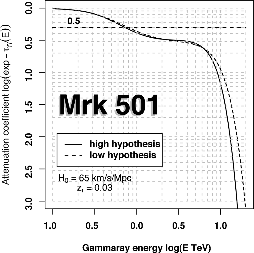
Figure 1: Synthetic absorption coefficients calculated for Mrk 501 ($z_{s}\sim 0.034$, $H_{0}=65\ \rm km\,s^{-1}\,Mpc^{-1}$). Solid curve (high hypothesis) takes into account the 100 and 60$\ \mu$m flux reported where dashed curve (low hypothesis) does not.

where $\epsilon_{\rm th}=2/(1-\mu)\epsilon_{1}$, $H_{0}$ is the Hubble parameter (assumed equal to $65\ \rm km\,s^{-1}\,Mpc^{-1}$ throughout this paper), and $n_{\rm DIrB}$ the density of the DIrB photon field. We have estimated this density by performing a Chebyshev interpolation using the measurements data compiled by Hauser & Dwek (2001) excluding the two points of COBE-DIRBE at $60\ \mu\rm m$ and $100\ \mu\rm m$. But note that with or without these points, the resulting absorption coefficients are quite similar above 9 TeV as shown in figure 1 and do not change the main results of this work.

2.4 Pair production rate and pair cascade

As mentioned above, the kinetic equation source term includes the contribution of the population of created particles in the pair production process as calculated above. Remarking that a hard photon with a reduced energy $\epsilon>1$ interacts preferentially with a soft photon of energy $\sim 1/\epsilon<1$ to form a pair $\rm e^{+}/e^{-}$ close to the production threshold. Consecutively, both particles have thus a similar energy $\gamma$ and we formally write the conservation of energy as $\epsilon+1/\epsilon\approx\epsilon=2\gamma$. Then the pair production rate reads

$$Q_{\rm prod}(\gamma;t)=\frac{{\rm d}N}{{\rm d}t{\rm d}\gamma{\rm d}V}\approx 2\dot{n}_{{\rm abs}}(\varepsilon=2\gamma;t).$$ (22)

Assuming the IC emission is isotropic in the plasma rest frame, the differential photon absorption rate density per energy and time unit, is given by

$$\dot{n}_{{\rm abs}}(\epsilon)=4\pi m_{e}c^{2}\frac{j_{\nu}}{h^{2}\nu}\mathscr{P}_{{\rm abs}}(\nu;t),$$ (23)

and we finally obtain

$$Q_{\rm prod}(\gamma;t)=\frac{8\pi m_{e}c^{2}}{h^{2}}\left[\frac{j_{\nu}}{\nu}\mathscr{P}_{{\rm abs}}(\nu;t)\right]_{\nu=2\gamma m_{e}c^{2}/h}.$$ (24)

2.5 Time-averaged spectra

At time $t$, the whole specific intensity in the plasma rest frame reads,

$$\mathscr{I}_{\nu}(\nu;t)\sim R\left[j_{S}(\nu;t)+j_{C}(\nu;t)\cdot\mathscr{C}_{\rm abs}(\nu;t)\right]\cdot\mathscr{C}_{\rm abs}^{\rm ext}(\nu,z_{s}),$$ (25)

where all parameters and emission coefficients are expressed above. All the physical quantities must be converted from the blob frame to the observer frame, taking into account the Doppler boosting effect and the cosmological corrections according

$$\tilde{\mathscr{F}}_{\tilde{\nu}}(\tilde{\nu};t)\sim\pi\dfrac{R^{2}}{d_{\ell}^{2}}\delta_{B}^{3}(1+z_{s})\mathscr{I}_{\nu}(\nu;t)\text{ with }\nu=\frac{1+z_{s}}{\delta_{B}}\,\tilde{\nu},$$ (26)

where $d_{\ell}$ is the usual luminosity distance, $\delta_{B}=1/\Gamma_{B}(1-\beta_{B}\cos\theta)$ is the Doppler beaming factor of the source and $\theta$ the viewing angle.
The observed spectrum is finally obtained by assuming that an observation takes place in the interval $[\tilde{t}_{\rm obs},\tilde{t}_{\rm obs}+{\Delta\tilde{t}}_{\rm obs}]$ (time $t=0$ is related to the beginning of the injection of fresh particles). The time-averaged spectrum is then

$$\tilde{\mathscr{F}}_{\tilde{\nu}}^{\rm obs}(\tilde{\nu})=\langle\tilde{\mathscr{F}}_{\tilde{\nu}}(\tilde{\nu})\rangle_{\tilde{t}}={1\over\tilde{\Delta t}_{\rm obs}}\int_{\tilde{t}_{\rm obs}}^{\tilde{t}_{\rm obs}+\tilde{\Delta t}_{\rm obs}}\tilde{\mathscr{F}}_{\tilde{\nu}}(\tilde{\nu};\tilde{t})\ {\rm d}\tilde{t}.$$ (27)

3 Results and discussion

3.1 General behavior

Our model requires eight parameters. Three of them are related to the properties of the source, namely the magnetic field strength $B\ \rm$, the radius $R$ (or $R_{15}$ when expressed in unit of $\rm 10^{15}\,cm$) and the bulk Doppler factor $\delta_{B}$. Three others characterize the injected plasma: they are the characteristic Lorentz factor of the ‘pile-up’ EDF $\gamma_{\rm max}$, the number of injected particles which can be characterized by the integrated Thomson optical depth $\tau_{\rm Th}=R\sigma_{\rm Th}\int{\rm d}t\int{\rm d}\gamma Q_{\rm inj}(\gamma;t)$ and the injection time $t_{\rm inj}$. The remaining parameters are the observational ones, ${t}_{\rm obs}$ and ${\Delta t}_{\rm obs}$.
In a steady-state model, there would only be five parameters since the last three ones would be irrelevant. More exactly the integrated Thomson optical depth $\tau_{\rm Th}$ should be replaced by the constant particle optical depth $\tau_{\rm Th}^{s}=nR\sigma_{\rm Th}$, where $n$ is the particle density in the source. For a ‘pile-up’ distribution, and neglecting pair creation, the whole spectrum is entirely characterized by two peak energies and two corresponding fluxes, corresponding respectively to the synchrotron and the IC bumps. Thus there would be only one free parameter left, which can be taken for instance as the unknown Doppler factor $\delta_{B}$ . Exactly the same spectrum would be obtained by varying $\delta_{B}$ and adjusting the other parameters accordingly. Since the TeV emission is dominated by the Klein-Nishina cut-off, the IC peak energy is simply proportional to $\delta_{B}\gamma_{\rm max}$, whereas the synchrotron peak energy is proportional to $\delta_{B}\gamma_{\rm max}^{2}B$. Thus the following scaling laws would apply :

$$\begin{array}[]{rcl}\gamma_{\rm max}&\propto&\delta_{B}^{-1},\\ B&\propto&\delta_{B}.\end{array}$$ (28)

The integrated synchrotron luminosity scales as $N\gamma_{\rm max}^{2}B^{2}\delta_{B}^{4}$, where $N=4\pi R^{3}n/3=4\pi\tau_{\rm Th}^{s}R^{2}/(3\sigma_{\rm Th})$ is the total number of particles in the source. So one gets the other following scaling law :

$$R^{2}\tau_{\rm Th}^{s}\propto\delta_{B}^{-4}.$$ (29)

The final condition must be determined by the fact that the IC luminosity $L_{\rm IC}$ is directly related to the synchrotron photon density in the source, which is itself directly related to the radius of the source (the synchrotron luminosity does not depend on this radius for a given number of particles). The magnetic energy density scales as $B^{2}$ so as $\delta_{B}^{2}$ (equation (28)), whereas the synchrotron photon energy density scales as $L_{\rm IC}\delta_{B}^{-4}R^{-2}$. If one neglects the Klein-Nishina correction, the ratio of synchrotron to Compton luminosity is simply the ratio of magnetic to soft photon density,and is fixed by the observations. One would thus expect the following scaling law

$$R\propto\delta_{B}^{-3}.$$ (30)

In fact the real condition is more involved because the Klein-Nishina cut-off diminishes strongly the number of photons effectively available for IC scattering, in a way depending on the Doppler factor and the shape of the synchrotron spectrum. But qualitatively, one can always choose the radius of the source to adjust the IC luminosity to the observed value.
There is however a limitation to the Doppler factor due to the existence of pair creation process. For to small values of $\delta_{B}$, the $\gamma-\gamma$ optical depth, can increase so much that it becomes of the order of unity. Then the IC luminosity stops increasing, and rather it starts to decrease with decreasing radius because of $\gamma-\gamma$ absorption. For a given Doppler factor, there is thus a maximum reachable IC luminosity. Conversely for a given IC luminosity, there is a minimum Doppler factor (which can be of course 1 in some cases where pair creation is never important). Note that the variability time scale is also a possible limitation, rapid variability requiring also high Lorentz factors.
In principle the time-dependent model is more constrained. It requires three more free parameters (the injection time and the two observation times), but the entire shape of the synchrotron spectrum is depending on these times. One can see that by varying $\delta_{B}$, the cooling time of particles with the typical energy $\gamma_{\rm max}$ varies as $(\gamma_{\rm max}B^{2})^{-1}\propto\delta_{B}^{-1}$ in the blob frame, so as $\delta_{B}^{-2}$ in the observer frame. The shape of the synchrotron spectrum will remain unchanged if one scales all times proportionally to $\delta_{B}^{-1}$ in the blob frame, or $\delta_{B}^{-2}$ in the observer frame. However, one of these times, namely the observation lasting time ${\Delta\tilde{t}}_{\rm obs}$ is not a free parameter. Thus if the model fits perfectly well the data for all values of $\delta_{B}$, only one of these values is compatible with the actual value of ${\Delta t}_{\rm obs}$. So theoretically a unique set of parameters (if any) can fit the data. Of course things are not so ideal : because of observation error bars, data will be fitted by a set of possible values with a satisfactory $\chi^{2}$ test.

3.2 Approximated analytical solution of the kinetic equation

For illustrative purposes, we develop here the simplest case where one can neglect the Inverse Compton cooling in comparison with the synchrotron cooling, and where pair production is unimportant. We can express analytically the general solution of equation (2) which satisfies the boundary condition $n_{\pm}(\gamma;t=0)=0$ for any arbitrary injection term $Q_{\rm inj}(\gamma;t)$ by,

$$n_{\pm}(\gamma;t)=\dfrac{1}{\left|\dot{\gamma}(\gamma)\right|}\int_{\gamma}^{\infty}{\rm d}\gamma_{0}\,Q_{\rm inj}\left(\gamma_{0};t-\tau(\gamma_{0},\gamma)\right),$$ (31)

where $\tau(\gamma_{0},\gamma)$ is the energy drift time, i.e. the time needed for a particle of energy $\gamma_{0}$ to cool down to the energy $\gamma$,

$$\tau(\gamma_{0},\gamma)=\int_{\gamma_{0}}^{\gamma}\dfrac{{\rm d}u}{\dot{\gamma}(u)}.$$ (32)

For the injection term chosen as in equation (3), equation (31) can be analytically integrated and we finally obtain,

$$n_{\pm}(\gamma;t)=\dfrac{n_{0}\gamma_{\rm max}^{3}}{k_{\rm syn}\gamma^{2}}\left[\Gamma\left(3,{a(\gamma;t)\over\gamma_{\rm max}}\right)-\Gamma\left(3,{b(\gamma;t)\over\gamma_{\rm max}}\right)\right],$$ (33)

where $\Gamma(\cdot,x)$ denotes to the incomplete gamma function.
Here the parameters $a(\gamma;t)$ and $b(\gamma;t)$ represent respectively the lower and upper bounds of the integral (31), where the integrand does not vanish. To evaluate them, we distinguish three time intervals for each value of $\gamma$. Let us define the parameter $t_{\rm cool}(\gamma)=|{\rm d}\gamma/{\rm d}\dot{\gamma}|=1/\gamma k_{\rm syn}$. Note that $t_{\rm cool}(\gamma)=\tau(\infty,\gamma)$, i.e. it represents also the time spent by an initial infinite energy particle to cool down to $\gamma$.
1.   Initial stage where $t<\min(t_{\rm cool}(\gamma),t_{\rm inj})$

$$b(\gamma;t)=\dfrac{\gamma}{1-k_{\rm syn}\gamma t}\quad;\quad a(\gamma;t)=\gamma.$$

Particles are still injected at the energy $\gamma$ but high energy particles have not yet cooled down to $\gamma$. Particles injected between $\gamma$ and some finite upper bound contribute to the integral.
2.   Cooling stage where $\max(t_{\rm inj},t_{\rm cool}(\gamma))<t<t_{\rm inj}+t_{\rm cool}(\gamma)$

$$b(\gamma;t)\to\infty\quad;\quad a(\gamma;t)=\dfrac{\gamma}{1-k_{\rm syn}\gamma(t-t_{\rm inj})}.$$

Particles are no more injected but some high energy particles are still cooling down to $\gamma$. Particles injected above a finite energy (larger than $\gamma$) contribute to the integral.
3.   Intermediate stage. For intermediate values of $t$, we must distinguish two specific energy ranges. We define a critical value of the individual Lorentz factor of the particles, $\gamma_{\rm lim}=1/k_{\rm syn}t_{\rm inj}$:
   3.a)   low energy range where $\gamma<\gamma_{\rm lim}$ (or $t_{\rm inj}<t_{\rm cool}(\gamma)$),

$$b(\gamma;t)=\dfrac{\gamma}{1-k_{\rm syn}\gamma t}\quad;\quad a(\gamma;t)=\dfrac{\gamma}{1-k_{\rm syn}\gamma(t-t_{\rm inj})}.$$

Injection is finished but very high energy particles have not yet cooled down to $\gamma$. Particles injected in some interval above $\gamma$ contribute to the integral.
   3.b)   high energy range where $\gamma\geqslant\gamma_{\rm lim}$ (or $t_{\rm inj}\geqslant t_{\rm cool}(\gamma)$),

$$b(\gamma;t)\to\infty\quad;\quad a(\gamma;t)=\gamma.$$

Conversely, very high energy particles have time to cool down to $\gamma$ while injection of fresh particles still takes place. All particles injected above $\gamma$ contribute. Note that this is the only stage for which $n(\gamma;t)$ does not depend on time. A steady-state is set during this stage (although not in the spectrum because the whole distribution is not steady).

We could also define an end stage for which $t>t_{\rm cool}(\gamma)+t_{\rm inj}$ and where $n_{\pm}(\gamma)=0$.

Introducing the reduced variables, $\varepsilon={\gamma}/{\gamma_{\rm max}}$ and $\tau_{i}={t_{i}}/{t_{\rm cool}(\gamma_{\rm max})}$, the previous equations can be collected into the following relation,

$$n(\varepsilon;\tau)=\dfrac{n_{0}\gamma_{\rm max}^{3}}{k_{\rm syn}\gamma^{2}}\,\varpi_{\tau_{\rm inj}}(\varepsilon;\tau),$$ (34)

where

$$\varpi_{\tau_{\rm inj}}(\varepsilon;\tau)=\varepsilon^{-2}\Theta(1-\varepsilon\max(0,\tau-\tau_{\rm inj}))\times\\ \quad\times\left[\Gamma\left(3,\dfrac{\varepsilon}{1-\varepsilon\max(0,\tau-\tau_{\rm inj})}\right)-\Theta(1-\varepsilon\tau)\Gamma\left(3,\dfrac{\varepsilon}{1-\varepsilon\tau}\right)\right].$$ (35)

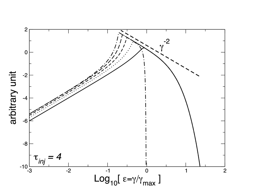
Figure 2: An example of resulting cooling ‘pile-up’ energy distribution function $\varpi_{\tau_{\rm inj}}(\varepsilon;\tau)$ for $\tau_{\rm inj}=4$ a time $\tau=1,2,3,4,5$. Also represented, in dashed straight line, a power-law of index 2 typical which results from the radiative cooling of a mono-energetic particle energy distribution.

An example of a resulting cooling pair-EDFs at different times is plotted in figure 2. One clearly sees the initial stage where the EDF is built, the formation of a $\gamma^{-2}$ EDF due to the cooling and the subsequent cooling of the whole distribution after the injection has stopped. As we will see in realistic simulations, the shape is however strongly modified when taking into account the IC cooling process (which is not simply dependent on the energy because of the Klein-Nishina cut-off) and the pair production term.

3.3 Application to Mrk 501 data

3.3.1 Observations

We have applied the model to fit the spectral energy distribution of Mrk 501 during the period of 1997 April when this source experienced an intense period of activity. From this period, we distinguish two different activity states, namely the ‘high state’ from the April 16 and the ‘medium state’ form the April 7. Simultaneous data are taken from BeppoSAX for the X-ray observation (Pian et al., 1998) and from the French Atmospheric $\check{\rm C}$erenkov Telescope $\check{\rm C}$AT for the spectrum in the TeV energy regime (Djannati-Ataï et al., 1999; Barrau et al., 1998). In a first step, we have corrected the high energy spectra using the attenuation coefficient computed previously. Note that the last corrected data point of the high state may be not meaningful, leading to a concave up corrected high energy spectrum. The most simply and obvious explanation of this problem is an over estimation of the measured high energy tail of the blazar spectrum or/and of the DIrB density itself.
The value of the $\Delta\tilde{t}_{\rm obs}$ is constrained by the observing duration. However there are some discontinuities in the observing time, which make the global observation period length different from the real exposure time. We have assumed that on average our $\Delta\tilde{t}_{\rm obs}$ corresponds to the global observing time of the BeppoSAX instruments LECS/MECS and PDS ($\sim$40000 s for the April 16, 37845 s for the April 7).

3.3.2 Solutions without pair creation

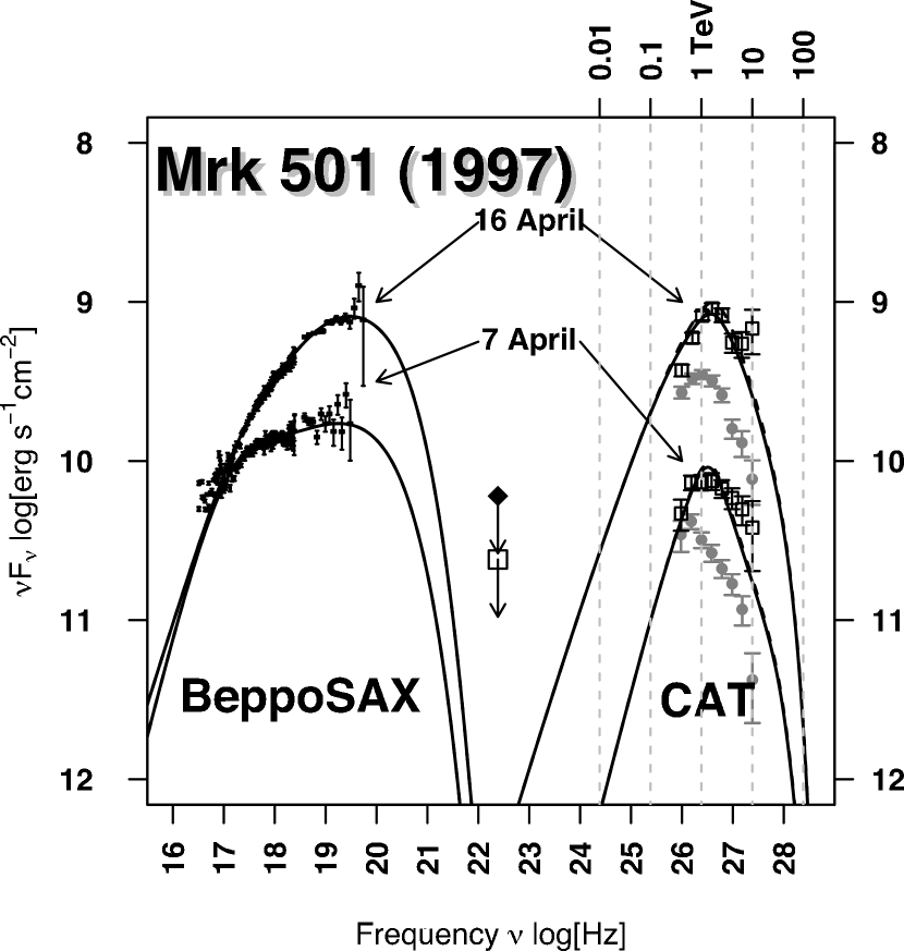
Figure 3: Fits of Mrk 501 data during the flaring period in 1997 April by the model. See Table 1 for the detail of the parameters values. For each state, the solid curves show the emergent spectrum modified by the intrinsic absorption due to the pair creation process in the spherical blob. The dashed curves show the unabsorbed one. Filled gray circles : observed $\check{\rm C}$AT data. Open squares : data corrected from the DIrB attenuation.

We can reproduce the data with parameters corresponding to almost no pair creation. The parameters used to fit the data are reported in Table 1 and the resulting synthetic SED are plotted in Figure 3. The fits are quite satisfactory for the high energy part of the SED. One-zone models are appropriate only to to reproduce this high energy, variable part. They can not account for the radio emission produced at much larger scale, where the whole jet contributes, possibly being the superposition of many successive flaring events.
In some range of Lorentz factor, a steady-state solution corresponding to $\gamma^{-2}$ power-law (see equation (33), case 3.b)) can be observed giving a $\nu^{-1/2}$ synchrotron flux index. This corresponds to the main part of the April 16 spectrum and and the low energy part of the April 7 one. Above this range, the spectrum is modified by a factor $t_{\rm cool}/t_{\rm obs}$ because the particles have cooled before the end of the observation. This produces a steepening of the spectrum by $\Delta\alpha=0.5$ and explains the flat high energy part of the synchrotron spectrum. The position of the spectral break is thus directly determined by the ratio between the cooling and the observation time. We obtain values of the magnetic field and of the transverse radius of the source ($R_{15}\sim 1$) in agreement with other models (see e.g. Bednarek & Protheroe, 1999; Tavecchio et al., 2001; Ghisellini, Celotti, & Costamante, 2002; Katarzyński et al., 2001; Konopelko et al., 2003). It turns out that this minimum Doppler factor implied by $\gamma-\gamma$ absorption in steady state models is quite high for Mrk 501, as noticed already by several authors. When the IC luminosity is corrected from extrinsic absorption, it can be as high as 50 for stationary models (see e.g. Bednarek & Protheroe, 1999; Konopelko et al., 2003). In the time dependent model, the constraint is somewhat released because high energy photons (TeV) are not produced at the same time as low energy, IR photons that are mainly responsible for their absorption. So the actual density of soft photons during the emission of highest energy TeV photons is lower than that measured on average. We see that good fits can be obtained with Doppler factors around 25, which implies a bulk Lorentz factor larger than 12. Not that this still relatively high value is necessary due to the correction of the spectra from from the DIrB absorption. These high values are generally in conflict with other features of TeV BL Lacs ; first VLBI/VLBA sub-parsec observations of Mrk 501 and others TeV blazars which don’t exhibit superluminal velocities at mas scale or excess in the derived synchrotron brightness temperature (Edwards & Piner, 2002; Piner & Edwards, 2004). Moreover, if we suppose that BL Lacs are the beamed counterparts of the FR-I radio galaxies, the ratio of their bolometric luminosity should be of the order of $\delta_{B}^{8}$. A $\delta_{B}$ larger than 10 would result in a much larger contrast than what is observed (Urry & Padovani, 1995). The spatial density of beamed vs unbeamed objects seems also to be better consistent with a Lorentz factor of around 3. All these argument disfavour a high Lorentz factor. This is in fact a problem inherent to any one zone model. We will argue in a future work (Saugé & Henri in preparation) than inhomogeneous models may solve this issue.

Like $B$ and $\delta_{B}$, $\gamma_{\max}$ is kept constant between the two different states. In the light of our scenario, the ‘medium state’ spectrum could be due to a previous ejection observed in a later stage (with respect of the injection time) than the April 16 one and in a much larger part of the jet.

We can also estimate the minimum variability time scale deriving from standard causality arguments and given by $\tilde{t}_{\rm var}>\tilde{t}_{\rm var,min}=555\,R_{15}\,(1+z_{s})\delta_{B}^{-1}\ \rm min$. Its value is reported in the last column of the Table 1 and is equal to 15 min for the high state and roughly 40 min for the medium state where the size of the source is much larger as mentioned above. Note however that the injection time is much larger than the above values.

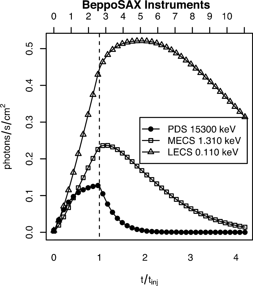
Figure 4: Mrk 501 April 16 simulated light curves for BeppoSAX instruments (left panel) and above 250 GeV (right pannel). Upper axis is graduated in unit of hours in the observer frame.

Simulated light curves corresponding to April 16 parameters are shown in figure 4. The curves are calculated for the 3 energy ranges of BeppoSAX and for very high energy (VHE) instruments above 250 GeV. Lags between various energy bands are clearly visible on the curves. Remarkably, the high energy photons lead the soft energy ones in the X-ray synchrotron component. but the high energy gamma-ray curve lags the synchrotron component. This is due to the fact that when particle distribution cools, the photon density below the Klein-Nishina limit increases. This makes the IC emission level keep rising even after the injection has stopped. Precise comparisons with observed light curves have not been made because the statistics is too poor to allow a meaningful analysis. However we can see qualitatively that complex temporal effects can arise from a time-dependent simulation leading to apparently contradictory behaviours. Note that whereas the presented simulations span the whole temporal interval of BeppoSAX observations, high energy observations have been performed only during a limited time within this interval. If they have taken place around the maximum of the light curve, few variations are expected.

Of course, a more realistic model could include a succession of different flares as well as a variation of the injection characteristic energy. This is however beyond the scope of this paper which only aims at showing that ‘pile-up’ particle energy distribution can well explain the high energy shape of TeV blazar spectra.

3.3.3 Solutions with pair creation

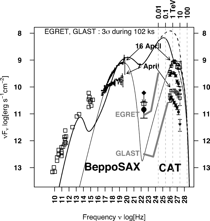
Figure 5: Time-averaged homogeneous one-zone SSC model for spectra of Mrk 501 in the case of an intense pair production. Thick grey lines show the EGRET and GLAST instruments sensitivity curve (3$\sigma$ during 102 ks).

Interestingly, we found also possible solutions with a much lower bulk Doppler factor, and accordingly a lower magnetic field, a higher particle Lorentz factor and a larger radius. An example of such parameters is shown in Table 2, and corresponding spectrum is displayed in figure 5. In this regime, pair production can be important. Although the IC flux should be much larger, the $\gamma-\gamma$ absorption reduces effectively the luminosity so that it can be compatible with the observations. The intense creation of new particles produces more synchrotron photons, which accelerates the cooling. This phenomenon also amplifies the effect of the increase of the Klein-Nishina threshold energy. This leads eventually to a catastrophic pair production/cooling process, producing a strong flare at GeV energy and in low energy X-rays. It explains the bump occuring in the GeV/sub-TeV energy range (and to a lesser extent in the radio sub-millimeter range). The flare is also more clearly visible on the light curves (figure 6) appearing as a very sharp flare in some energy ranges. Although the relevance of such scenario is not clear, it may be possible that such events could explain the most rapid variations in the TeV light curves. The GeV flare would have been in principle observable by the EGRET instrument. However due to the small number of simultaneous EGRET/TeV observations and the briefness of the event, it could have escaped any detection. We note also that for different value of the parameters, it is possible that the X-ray flare shifts toward lower energy, disappearing from the X-ray data. This could be related to the ‘orphan flare events’ observed in some occasions (Krawczynski et al., 2004).

4 Conclusion

This paper shows that the high energy spectra of TeV blazars can be well reproduced by a cooling ‘pile-up’ EDF. This offers an alternative to the narrow power-law injection terms often used in the literature, whose justification is unclear. Inclusion of time-dependent effects permits to reproduced the main features of both the light curves and the time-averaged spectra. For a given SED shape, the parameters of the model are fully constrained. For Mrk 501, different states could be the result of the time variation of the transverse radius of the source $R$, the quantity of injected leptons via $\tau_{\rm Th}$ and the observational parameters with respect of the injection time. However, this one zone model shares a common issue with other homogeneous models : it requires high values of the bulk Lorentz factor to avoid a strong gamma-ray absorption, even in the case of the optically thick solution (see section 3.3.3). These high Lorentz factors appear to be inconsistent with those deduced from FR I/BL Lacs unification models (Urry & Padovani, 1995; Chiaberge et al., 2000). They are also difficult to reconcile with the absence of superluminal motion at TeV scale and relatively low brightness temprature of TeV blazars (Edwards & Piner, 2002; Piner & Edwards, 2004). We will argue in a future work that inhomogeneous models could fix this issue.

Appendix A An accurate analytic approximation of pitch angle averaged
synchrotron emitted power

As mentioned in section 2.3.1, the $R_{{\rm CS}}(x)$ function (see equation7) results from the monochromatic emitted power averaged on a population of particles with randomly distributed pitch angle. It mathematically reads (Crusius & Schlickeiser, 1986)

$$R_{{\rm CS}}(x)=\frac{1}{2}\int_{0}^{\pi}{\rm d}\theta\,\sin^{2}\theta F_{{\rm syn}}\left(\frac{x}{\sin\theta}\right),$$ (A1)

where $F_{{\rm syn}}(x)$ is the usual synchrotron fundamental kernel (Blumenthal & Gould, 1970),

$$F_{{\rm syn}}(x)=x\int_{x}^{\infty}{\rm d}z\,K_{5/3}(z).$$ (A2)

For $x\ll 1$ approximate expression of $F_{{\rm syn}}$ is

$$F_{{\rm syn}}(x)\approx\text{ $\frac{4\pi}{\sqrt{3}\Gamma(1/3)}\left(\frac{x}{2}\right)^{1/3}$}\quad,\quad x\ll 1.$$ (A3)

and we immediately obtain the relevant one for $R_{{\rm CS}}$,

$$R_{\ll}(x)=\frac{1}{2}\int_{0}^{\pi}{\rm d}\theta\,\sin^{2}\theta F_{{\rm syn}}\left(\frac{x}{\sin\theta}\right)=\frac{2^{1/3}}{5}\Gamma^{2}(1/3)x^{1/3}\approx 1.808418\,x^{1/3}.$$ (A4)

Conversely, for large argument ($x\gg 1$), the asymptotic development of $F_{{\rm syn}}$ is $\left.(\pi x/2\right)^{1/2}\mathrm{e}^{-x}$ and then

$$R_{\gg}(x)=\frac{1}{2}\int_{0}^{\pi}{\rm d}\theta\,\sin^{2}\theta F_{{\rm syn}}\left(\frac{x}{\sin\theta}\right)=\frac{1}{2}\left(\frac{\pi x}{2}\right)^{1/2}\int_{0}^{\pi}{\rm d}\theta\,\sin^{3/2}\theta\mathrm{e}^{-x/\sin\theta}.$$ (A5)

The preceding integral can re-writes as,

$$\mathcal{I}(x)=\int_{0}^{\pi}{\rm d}\theta\,\exp(-f_{x}(\theta))\quad,\quad f_{x}(\theta)=\frac{x}{\sin\theta}-\frac{3}{2}\ln(\sin\theta).$$ (A6)

Remarking that the exponential argument is symmetric around $\theta=\pi/2$ and therefore on the integration range, we set $\theta=\pi/2+\varphi$ and make a taylor expansion around $\varphi$

$$\tilde{f}_{x}(\varphi)=\frac{x}{\cos\varphi}-\frac{3}{2}\ln(\cos\varphi)\approx x+\frac{\varphi^{2}}{2}\left(x+\frac{3}{2}\right)+\mathcal{O}(\varphi^{3})$$ (A7)

Then integral (A6) rewrites,

$$\mathcal{I}(x)\approx\mathrm{e}^{-x}\int_{-\pi/2}^{\pi/2}{\rm d}\varphi\,\mathrm{e}^{-\varphi^{2}/2\sigma^{2}}\quad{\rm with}\quad 1/\sigma^{2}=x+\frac{3}{2},$$ (A8)

which is a standard gaussian integral. Noting that larger is $x$ sharper is the integral argument, lower and upper bound can be extended to infinity as $x\gg 1$ (error is less than $10^{-10}$ for $x\geqslant 3$ and ). We finally obtain,

$$R_{\gg}(x)=\frac{\pi}{2}\sqrt{\frac{2x}{x+3}}\mathrm{e}^{-x}.$$ (A9)

For intermediate values, we perform a polynomial fit of the form,

$$R_{{\rm int}}(x)=a_{0}(x^{a_{1}}+a_{2}x^{2a_{1}}+a_{3}x^{3a_{1}})\exp(-a_{4}x^{a_{5}}),$$ (A10)

where the coefficient $a_{i}$ is obtained from least square fitting and is given in table 2. In this regime, RMS error is in order of 0.05% .

Table 1: Mkn 501 physical fit parameters

	$B$	$R_{15}$	$\delta_{B}$	$\gamma_{\rm max}$	$\tau_{\rm Th}$	$\tilde{t}_{\rm inj}$	$\tilde{t}_{\rm obs}$	${\Delta\tilde{t}}_{\rm obs}$	$\tilde{t}_{\rm var,min}$
	(G)	$\rm\ (10^{15}\,cm)$		$10^{6}$	$10^{-10}$	(ks)	(ks)	(ks)	(min)
high state	0.077	0.65	25	1.26	58.5	9.4	3.29 ($=0.35\,\tilde{t}_{\rm inj}$)	39.7	15
medium state	0.075	1.75	25	1.29	8.95	40	35 ($=0.875\,\tilde{t}_{\rm inj}$)	37.8	40
‘GeV flaring state’	0.047	1.06	16	2	144.1	24.4	8.54 ($=0.35\,\tilde{t}_{\rm inj}$)	102	38

Table 2: Resulting fitting coefficients from the polynomial approximation of the function $R_{\rm CS}$

$a_{0}$ =	0.	201 447$\times 10$
$a_{1}$ =	0.	344 606
$a_{2}$ =	-0.	429 682
$a_{3}$ =	0.	273 331$\times 10^{-2}$
$a_{4}$ =	0.	966 844
$a_{5}$ =	0.	964 518
$\chi^{2}$ =	1.	27$\times 10^{-5}$
RMS % error =	0.	05

Figure 6: Same as figure 4 for the case of an intense pair production.

References

- Abramowitz & Stegun (1964) Abramowitz, M., & Stegun, I.A. 1964, Handbook of Mathematical Functions, Applied Mathematics Series - 55 (1965, New York: Dover Publication Inc.)
- Aharonian, Atoyan, & Nahapetian (1986) Aharonian, F. A., Atoyan, A. M., & Nahapetian, A. 1986, A&A, 162, L1
- Aharonian et al. (2002) Aharonian, F. et al. 2002, A&A, 384, L23
- Aharonian et al. (2003) Aharonian, F. et al. 2003, A&A, 406, L9
- Barrau et al. (1998) Barrau A. et al. 1998, Nucl. Instrum. Methods Phys. Res A, 416, 278
- Bednarek & Protheroe (1999) Bednarek, W. & Protheroe, R. J. 1999, MNRAS, 310, 577
- Blumenthal & Gould (1970) Blumenthal G., Gould R. 1970, Rev. Mod. Phy., vol 2, 2, 237
- Catanese et al. (1998) Catanese, M., et al. 1998, ApJ, 501, 616
- Catanese & Sambruna (2000) Catanese, M. & Sambruna, R. M. 2000, ApJ, 534, L39
- Chadwick et al. (1999) Chadwick, P., et al. 1999, ApJ, 513, 161
- Chiaberge et al. (2000) Chiaberge, M., et al. 2000, A&A, 358, 104
- Coppi & Blandford (1990) Coppi, P.S. & Blandford, R.D. 1990, MNRAS, 245, 453
- Crusius & Schlickeiser (1986) Crusius A., Schlickeiser R. 1986, A&A, 164, L6
- Djannati-Ataï et al. (1999) Djannati-Ataï, A. et al. 1999, A&A, 350, 17
- Djannati-Ataï et al. (2002) Djannati-Ataï, A. et al. 2002, A&A, 391, L25
- Dermer, Miller, & Li (1996) Dermer, C. D., Miller, J. A., & Li, H. 1996, ApJ, 456, 106
- Edwards & Piner (2002) Edwards, P. G. & Piner, B. G. 2002, ApJ, 579, L67
- Finkbeiner, Davis, & Schlegel (2000) Finkbeiner, D. P., Davis, M., & Schlegel, D. J. 2000, ApJ, 544, 81
- Georganopoulos & Kazanas (2003) Georganopoulos, M. & Kazanas, D. 2003, ApJ, 594, L27
- Ghisellini, Maraschi, & Treves (1985) Ghisellini, G., Maraschi, L., & Treves, A. 1985, A&A, 146, 204
- Ghisellini et al. (1988) Ghisellini, G., Guilbert P., Svensson R. 1988, ApJ, 334, L5
- Ghisellini, Celotti, & Costamante (2002) Ghisellini, G., Celotti, A., & Costamante, L. 2002, A&A, 386, 833
- Gould & Schréder (1967a) Gould, R. J. & Schréder, G. P. 1967a, Physical Review , 155, 1404
- Gould & Schréder (1967b) Gould, R. J. & Schréder, G. P. 1967b, Physical Review , 155, 1408
- Hauser & Dwek (2001) Hauser M.G., Dwek, E. 2001, ARA&A, 39, 249
- Henri & Pelletier (1991) Henri P., Pelletier G. 1991, ApJ, 383, L7
- Holder et al. (2003) Holder, J. et al. 2003, ApJ, 583, L9
- Horan et al. (2002) Horan, D., et al. 2002, ApJ, 571, 753
- Jones (1968) Jones F.C. 1968, Phys. Rev., 167, 1159
- Jones, O’dell, & Stein (1974) Jones, T. W., O’dell, S. L., & Stein, W. A. 1974, ApJ, 192, 261
- Jones (1994) Jones, F. C. 1994, ApJS, 90, 561
- Katarzyński et al. (2001) Katarzyński K., Sol H., Kus A. 2001, A&A, 367, 809
- Konigl (1981) Konigl, A. 1981, ApJ, 243, 700
- Konopelko et al. (2003) Konopelko, A. K., Mastichiadis, A., Kirk, J. G., de Jager, O. C., & Stecker, F. W. 2003, preprint (astro-ph/0302049)
- Krawczynski et al. (2004) Krawczynski, H., et al. 2004, ApJ, 601, 151, preprint (astro-ph/0310158)
- Lacombe (1977) Lacombe, C. 1977, A&A, 54,
- Marcowith, Henri & Pelletier (1995) Marcowith, A., Henri, G., & Pelletier, G. 1995, MNRAS, 277, 681
- Nishiyama et al. (2000) Nishiyama, T., et al. 2000, AIP Conf. Proc. 516, Proceedings of the 26th International Cosmic Ray Conference, ed. B.L. Dingus, D.B. Kieda & M.H. Salamon (Salt Lake City, Utah:AIP), 3, 370
- Pelletier (1985) Pelletier G. 1985, in proceedings “Plasma turbulence and Astrophysical Objects”, SFP
- Pelletier & Sol (1992) Pelletier G., Sol H. 1992, MNRAS, 254, 635
- Pian et al. (1998) Pian, E. et al. 1998, ApJ, 492, L17
- Piner & Edwards (2004) Piner, B. G. & Edwards, P. G. 2004, ApJ, 600, 115
- Punch et al. (1992) Punch, M., et al. 1992, Nature, 358, 477
- Protheroe & Stanev (1999) Protheroe, R. J. & Stanev, T. 1999, Astroparticle Physics, 10, 185
- Quinn et al. (1996) Quinn, J., et al. 1996, ApJ, 456, L83
- Rybicki & Lightman (1979) Rybicki, G. B. & Lightman, A. P. 1979, Radiative Processes in Astrophysics (New York: Wiley-Interscience)
- Schlickeiser (1985) Schlickeiser, R. 1985,A&A, 143, 431
- Stecker, de Jager & Salamon (1992) Stecker, F. W., de Jager, O. C., & Salamon, M. H. 1992, ApJ, 390, L49
- Tavecchio et al. (2001) Tavecchio, F. et al. 2001, ApJ, 554, 725
- Trussoni et al. (2003) Trussoni, E. el al. 2003, A&A, 403, 889
- Urry & Padovani (1995) Urry, C. M. & Padovani, P. 1995, PASP, 107, 803
- Vassiliev (2000) Vassiliev, V. V. 2000, Astroparticle Physics, 12, 217