The Star Clusters of the Small Magellanic Cloud:
Age Distribution

Abstract

We present age measurements for 195 star clusters in the Small Magellanic Cloud based on comparison of integrated colors measured from the Magellanic Clouds Photometric Survey with models of simple stellar populations. We find that the modeled nonuniform changes of cluster colors with age can lead to spurious age peaks in the cluster age distribution, that the observed numbers of clusters with age, $t$, declines smoothly as $t^{-2.1}$, that for an assumed initial cluster mass function scaling as $M^{-2}$ the dependence of the cluster disruption time on mass is proportional to $M^{0.48}$, that despite the apparent abundance of young clusters the dominant epoch of cluster formation was the initial one, and that there are significant differences in the spatial distribution of clusters of different ages. Because of limited precision in our age measurements, we cannot address the question of detailed correspondence between the cluster age function and the field star formation history. However, this sample provides an initial guide for which clusters to target in more detailed studies of specific age intervals.

1. Introduction

The discovery of young star clusters in ongoing galaxy mergers (Holtzman et al., 1992; Whitmore et al., 1993) has provided added motivation for understanding the formation mechanism of stellar clusters and the dynamical processes that lead to their destruction. While the ancient clusters in our own galaxy provide only indirect information regarding the formation or disruption of clusters, the Magellanic Clouds contain numerous young clusters ($<1$ Gyr old) for study (Hodge, 1961; van den Bergh, 1981). The large number of clusters is of great statistical value, but it has divided the studies into two camps. Ages have been determined either for large samples of clusters using low-precision measurements, such as integrated colors (for example see van den Bergh (1981)) or for small samples using high-precision measurements, such as color-magnitude diagrams (for an early example see Baird et al. (1974)). Each approach has its strengths and weaknesses, but a study of the overall population must include age estimates for a large fraction of all the clusters in the galaxy. Only with such measurements can one begin to address whether the cluster formation history tracks the field star formation history, how quickly clusters are dissolved, and whether the cluster system as a whole still retains some memory of cluster formation episodes.

The study of the clusters in the Magellanic Clouds has a rich history that cannot be properly summarized here. Nevertheless, from that work we know of several interesting features in the age distribution of clusters in both the Large and Small Magellanic Clouds (LMC and SMC). In the LMC there is an “age gap” (a deficit of clusters of ages corresponding to ages between roughly 3 and 10 Gyr) that has been extensively studied (Jensen et al., 1988; Da Costa, 1991; van den Bergh, 1991; Rich et al., 2001). The age distribution of clusters in the SMC is less established. Ground based studies of SMC clusters have concluded that the age distribution is continuous (Da Costa & Hatzidimitriou, 1998; Mighell et al., 1998), but analysis of the SMC’s seven brightest old (age $>1$ Gyr) clusters with the Hubble Space Telescope has suggested two distinct episodes of cluster formation that occurred 2 $\pm$ 0.5 Gyr and $8\pm 2$ Gyr ago (Rich et al., 2000). Three additional SMC clusters that satisfy the age criteria but are too faint to be included in the $HST$ study are Lindsay 1, which has a ground-based age of 9 Gyr and so is coincident with the older burst, Lindsay 11, which has an age of 3.7 Gyr, and Lindsay 113, which has an age of 5.3 Gyr (Mighell et al., 1998; Rich et al., 2000). Neither of the latter two appear to have formed within the two identified bursts and may populate the “gap”. Whether the structure in the age distribution is real, and whether it tracks any pattern observed in the field star formation history of the SMC, are open questions.

We present a study based on integrated colors of 195 clusters in the SMC that incorporates a number of improvements over similar previous studies: 1) we use digital imaging in four filters (most previous studies of integrated colors were based on photographic plates and utilized only two or three filters), 2) we use the structural parameters individually derived for each cluster (Hill & Zaritsky, 2003) to set our aperture size (most previous studies have a fixed aperture size for all clusters), and 3) we use multiple theoretical models of simple stellar populations to derive an age and associated uncertainty (most previous studies calibrated integrated colors to a small number of clusters with ages derived from color-magnitude diagrams — a procedure that can lead to coarse age resolution and unknown systematic problems that are difficult to explore, see §3.1). The data and methodology used to measure ages are described in §2. We discuss various aspects of the derived age distribution in §3 and summarize in §4.

2. Data and Analysis

2.1. Images of the Cluster Sample

The sample of SMC clusters that we analyze is presented by Hill & Zaritsky (2003). Coordinates and cross-identifications are given in Table 1. With the exception of clusters and associations embedded in the complex environment of star forming regions, these 204 clusters are the most unambiguous clusters in the 4.5${}^{\circ}\times 4^{\circ}$ section of the SMC observed by the Magellanic Clouds Photometric Survey (Zaritsky et al., 2002). Figure 1 shows images of clusters 1 through 16. We have excluded clusters and associations that lie within emission line nebulae because of the difficulty in measuring integrated colors in such an environment. The absence of these clusters explains in part why other catalogs list many more star clusters (for example see Pietrzyński et al. (1998) and Bica & Dutra (2000)), but we also found from visual inspection of over a thousand candidate clusters that many are quite marginal. It is not our contention that only the clusters presented here are real. There are almost certainly real clusters lurking among the previously published catalogs that we have excluded. However, even if real, we cannot confidently measure the colors or structural parameters of such poor clusters. When considering the results from our sample, one must remain aware that we are incomplete in both the youngest and poorest (poor in either total number of stars or surface density) clusters. The latter might be a particularly interesting population because it may consist of clusters that are nearing the end of their lifetime as bound objects.

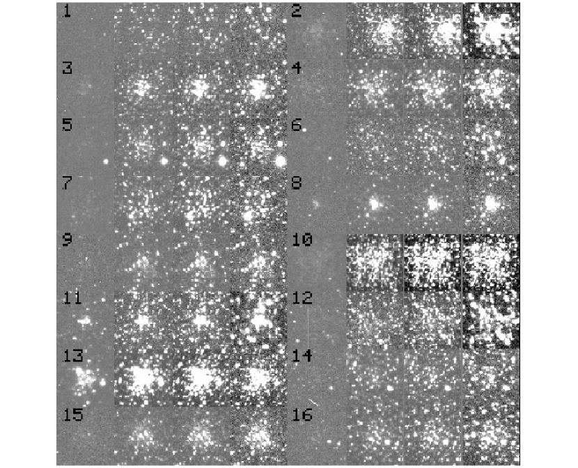
Figure 1.— $UBVI$ images of the clusters. Each row contains the four filter images for two clusters. The images are 70 arcsec on a side and oriented such that N is to the right and E to the bottom. This Figure includes the images for clusters 1 through 16. The remainder of the images are available in the electronic version.

Table 1CLUSTERS AND THEIR COLORS

Number	RA	DEC	$M_{V}$	$\sigma_{V}$	U$-$B	$\sigma_{U-B}$	B$-$V	$\sigma_{B-V}$	V$-$I	$\sigma_{V-I}$	Name
1	0 24 18.67	$-$73 59 35.8	15.92	1.17	0.75	0.24	0.72	0.14	0.92	0.07	$\cdots$
2	0 24 43.16	$-$73 45 11.7	$\cdots$	$\cdots$	$\cdots$	$\cdots$	$\cdots$	$\cdots$	$\cdots$	$\cdots$	K5, L7, ESO28-18
3	0 25 26.60	$-$74   4 29.7	14.23	$\cdots$	0.57	$\cdots$	0.65	$\cdots$	1.10	$\cdots$	K6, L9, ESO28-20
4	0 27 45.17	$-$72 46 52.5	13.95	0.38	0.03	0.09	0.80	0.04	1.20	0.05	K7, L11, ESO28-22
5	0 28   2.14	$-$73 18 13.6	14.85	1.17	0.28	0.05	0.61	0.05	1.00	0.40	K8, L12
6	0 29 55.22	$-$73 41 57.1	14.31	1.12	-0.05	0.48	0.65	0.06	0.37	0.32	HW3
7	0 30   0.26	$-$73 22 40.7	13.84	$\cdots$	0.54	$\cdots$	1.08	$\cdots$	1.32	$\cdots$	K9, L13
8	0 31   1.34	$-$72 20 30.0	14.64	0.28	0.00	0.04	0.80	0.07	1.20	0.12	HW5
9	0 32 41.02	$-$72 34 50.1	14.66	0.35	0.26	0.18	0.87	0.05	0.90	0.05	L14

Note. — The complete version of this table is at: http://ngala.as.arizona.edu/dennis/rafelski.html The printed edition contains only a sample.

Our cluster images are drawn from drift scan imaging of the central $4^{\circ}\times 4.5^{\circ}$ of the SMC in $U,B,V$, and $I$ done with the Las Campanas Swope telescope (1m) and the Great Circle Camera (Zaritsky et al., 1996) between 1996 November and 1999 December. The effective exposure time for any portion of the SMC is between 4 and 5 min and the pixel scale is 0.7 arcsec pixel^-1. A photometric catalog of stars is presented by Zaritsky et al. (2002), but in this study we use the reduced images rather than the stellar catalog because of the catalog’s incompleteness in the high-density centers of stellar clusters. We extract $350^{\prime\prime}\times 350^{\prime\prime}$ subimages in each of the four filters centered on the cluster from the larger drift scans. We use the photometric solutions that were applied to the stellar catalog, which have an observational scatter of between 0.01 and 0.04 mag for standard star fields. This uncertainty is significantly smaller than that resulting from other sources of error in the measurement of cluster integrated colors.

2.2. Integrated Cluster Colors

The measurement of an integrated color or magnitude depends critically on the degree to which one can subtract the effect of the underlying background. This is one area in which the availability of moderate resolution digital images should enable a quantitative improvement over previous studies. The two primary considerations are where to set the cluster and background apertures and how to remove contamination by stars that are too bright to be plausible cluster members or random SMC field stars (these are typically foreground Galactic stars).

The optimal choice of aperture size is not evident. The clusters in this sample vary significantly in size, so a single aperture size is inappropriate. Although the cluster’s tidal radius might be a natural choice for the outer scale of the aperture, the measurement of the tidal radius is highly uncertain. Hill & Zaritsky (2003) found that the radius that encloses 90% of the light of a cluster, $r_{90}$, is much less sensitive to uncertainties in defining the background level. We use their tabulated values of $r_{90}$ in the $V$ band to set our aperture size for each cluster independently. The apertures are circular and are the same for all filter bands. The background is calculated from the area of the $350^{\prime\prime}\times 350^{\prime\prime}$ cluster image that lies 5 pixels ($3.5^{\prime\prime}$) beyond $r_{90}$.

The effect of contamination in both the cluster and background apertures can be severe. We minimize the impact of the brightest stars on our calculation of the background by adopting an upper limit to the pixel values used in the calculation. First, we calculate the mean background, without this threshold. Then we set the threshold to be equal to the mean background level plus two times the central flux value of the cluster. Lastly, we calculate the mean background level using this threshold. The possibility of foreground contamination within the cluster aperture is smaller because its area is smaller than that of the background aperture. However, from visual examination we suspect that the photometry of as many as 73 clusters may be significantly contaminated by an unusually bright star for at least one of the filters within the aperture corresponding to the upper $1\sigma$ bounds on $r_{90}$. Because the measurement of the cluster luminosity is the integrated flux within the aperture, rather than an average, we cannot simply exclude high valued pixels. Instead we flag such clusters in Table 1 but do not correct their photometry. We found that these clusters do not have noticeably different properties than the others.

To arrive at the measurement of the cluster magnitude in each filter, we sum the counts within the $r_{90}$ cluster aperture, subtract the mean background level, multiply by 10/9 to correct for the choice of $r_{90}$ as the aperture, and iteratively apply the photometric solution to incorporate the color terms. Magnitudes and colors are presented in Table 1. To estimate uncertainties in these quantities, we recalculate the magnitudes and colors using the $1\sigma$ bounds on $r_{90}$. Hill & Zaritsky (2003) do not present $\sigma_{r_{90}}$ for some clusters because their best fit King model was not statistically acceptable. For these clusters we adopt the average of the color uncertainty calculated for the other clusters. The uncertainty from the photometric calibration is added in quadrature, but it is a minor contribution. Magnitudes and colors, in particular filter bands, are unavailable for the 35 clusters whose images are saturated in at least one of the filters, the two clusters that are off an edge of a scan, and the one cluster (number 180) whose image quality is too low to be useful. These problems often affect the cluster image in only one filter, and in such cases the magnitudes are calculated for the unaffected filters. There are 38 clusters that are missing at least one of the three colors in our Table 1, but only seven for which we are unable to compute any colors. Eliminating these seven plus the two that are off the edges of scans leaves us with 195 clusters, out of the original 204, for which we measure an age.

Because contamination is such a serious problem, and because, as we will show below, the integrated colors scatter widely around the model predictions, we investigate whether adopting a smaller cluster aperture would lead to more robust colors. Using colors from small apertures assumes that there are no internal color gradients. We re-measure colors using an aperture of radius $0.5r_{90}$ and find no noticeable decline in the scatter of the colors about the model predictions. We conclude that the contamination cannot be significantly mitigated by decreasing the aperture, partially because the scatter is also due to stochastic effects within the cluster’s own population.

We obtain an external estimate of the measurement uncertainties by comparing our magnitudes and colors to previous studies where possible. A compilation of integrated colors from various photometric studies is presented by van den Bergh (1981). Figures 2 and 3 show the differences between our V magnitudes and colors and those tabulated by van den Bergh (1981). The error bars are underestimated because they do not include the uncertainties in the compiled data (none were quoted). Assuming a standard error of 0.1 mag, the scatter in $B-V$ appears to be entirely consistent within the uncertainties, while it appears that we have slightly underestimated the uncertainties in $U-B$ (either in our data or van den Bergh’s). In the mean both colors agree well. To quantitatively determine whether the scatter is commensurate with the quoted uncertainties, we examine the distributions of $\Delta$color/$\sigma$. If the uncertainty estimates are correct, a Gaussian fit to the distribution should have $\sigma=1$. Instead, we find (after removing the mean offset, one highly discrepant cluster, and not adopting any uncertainties for the published data) that the fit has a dispersion that is $\sim 1.5$. However, if the uncertainties in the published data are similar to ours, then $\sigma_{\Delta}$ would be 40% larger than calculated and the fitted Gaussian would have a dispersion that is close to one. We conclude that except for the offset in the mean, our colors are statistically consistent with previous measurements and our uncertainty estimates are appropriate.

Figure 2.— Comparison of our V magnitudes, $V_{R}Z$, with those from van den Bergh (1981), $V_{V}dB$. The van den Bergh (1981) compilation did not quote photometric uncertainties, and thus only uncertainties in our measurements are shown. The errorbars correspond to those in the tables. The line is the 1:1 correlation.

Figure 3.— Comparison of our $B-V$ and $U-B$ colors with those from van den Bergh (1981). The difference is our values - van den Bergh (1981). The van den Bergh (1981) compilation did not quote photometric uncertainties, and thus only uncertainties in our measurements are shown. The errorbars correspond to those in the tables.

2.3. Determining Cluster Ages

The integrated colors of any stellar population provide a luminosity weighted age measurement. The color should be a particularly stable chronometer for clusters because they formed their stars over a timescale that is much shorter than their age. We can measure the age of a cluster to the degree that we can accurately measure and model the colors. The colors are presented in Table 1 and the models we use are those of Leitherer et al. (1999), hereafter referred to as the Starburst99 or S99 models, and of Anders and Fritze-v. Alvensleben (2003), hereafter referred to as the GALEV models. The S99 models that we use correspond to the standard mass loss prescription, the theoretical wind model, and the full isochrone mass interpolation. We have adopted a Salpeter IMF in both models. We derive ages using models with a range of appropriate metallicites ($Z=$ 0.001, 0.004, and 0.008 for the S99 models and 0.004 and 0.008 for the GALEV models). These metallicity values refer to the mass fraction of metals relative to hydrogen and correspond to [Fe/H] of $-$1.3, $-$0.7, and $-$0.4, respectively. Observations of individual clusters (Dopita et al., 1985; Da Costa, 1991; Pagel & Tautvais̆ienė, 1998; de Freitas Pacheco et al., 1998; Piatti et al., 2001) and the reconstruction of the global chemical enrichment history of the SMC from color-magnitude diagrams (Harris & Zaritsky, 2004) suggest that the metallicity of the SMC has for the most time varied between [Fe/H] $\sim-1.2$ and $-0.4$. As we discuss below, some of the finer details of the cluster formation history are extremely sensitive to the exact choice of metallicity for the model and our current constraints on the age-metallicity relationship are insufficiently precise to dictate which model should be used for each age.

In Figures 4, 5, and 6 we overlay the two sets of models over our reddening-uncorrected cluster colors. We find a mean agreement with the S99 models, although the observational scatter is large. The principal systematic difference between our data and the models appears to be in the $V-I$ colors (which are too red in the models for the bluest clusters). The general agreement of the $B-V$ colors suggests that the problem lies in the modeling of the $I$-band. The agreement is significantly poorer relative to the GALEV models, but we continue to use those models as well to examine systematic errors introduced into the derived ages by the use of one or the other set of theoretical models.

Figure 4.— Integrated $U-B$ vs $B-V$ from data and models for SMC clusters. The triangles represent our measurements, the points, which blend into a line in certain regions, represent the Starburst99 model for Z = 0.004 (for ages between 0.001 and 10 Gyrs), and the line represents the GALEV model for Z = 0.004 (for ages between 0.004 and 14 Gyrs).

Figure 5.— Integrated $V-I$ vs $B-V$ from data and models for SMC clusters. The triangles represent our measurements, the points, which blend into a line in certain regions, represent the Starburst99 model for Z = 0.004 (for ages between 0.001 and 10 Gyrs), and the line represents the GALEV model for Z = 0.004 (for ages between 0.004 and 14).

Figure 6.— Integrated $U-B$ vs $V-I$ from data and models for SMC clusters. The triangles represent our measurements, the points, which blend into a line in certain regions, represent the Starburst99 model for Z = 0.004 (for ages between 0.001 and 10 Gyrs), and the line represents the GALEV model for Z = 0.004 (for ages between 0.004 and 14).

The observed scatter of the colors about the theoretical model is the fundamental observational limit to the precision with which we can measure ages. The scatter arises from a variety of sources including the lack of a reddening correction, which we discuss below, stochastic effects within the cluster population, contamination of the cluster apertures, which we discussed in §2.2, and the contamination of the background aperture, which we attempt to minimize. The last three of these possibilities will become less important as we consider intrinsically brighter clusters. A comparison (Figure 7) between our $U-B$, $B-V$ colors and those presented by van den Bergh (1981), shows that indeed for these clusters, which are among the most luminous clusters, the scatter about the model line (in particular the S99 model) is much smaller than for the sample as a whole (Figure 4). We note, however, that the difference between the two models is often comparable to the scatter in the data.

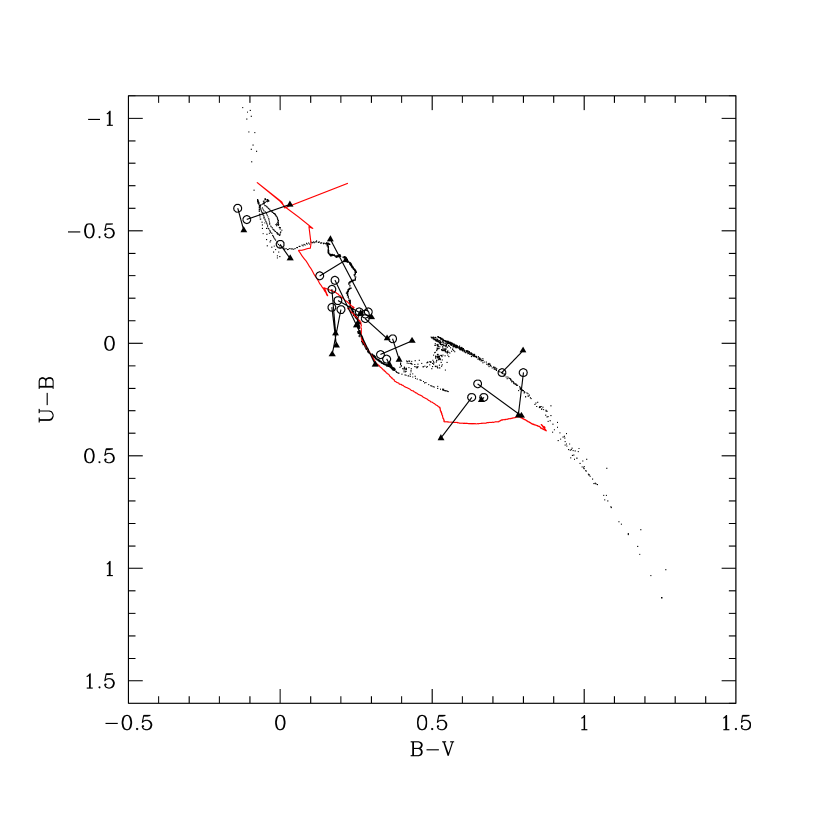
Figure 7.— Comparison of our color measurements (triangles) to those of van den Bergh (1981) (circles). Straight lines connect the measurements for the same cluster. The models are as in Figures 4 - 6.

To measure a cluster’s age, we calculate the color difference between data, typically $U-B$, $B-V$ and $V-I$, although not all colors are available for all clusters (see §2.2), and models, at all ages available for the particular model. At each age, $\chi^{2}$ is evaluated using all the available colors and we adopt the age that corresponds to the minimum $\chi^{2}$. Age limits corresponding to the 90% confidence range are derived using the criterion that $\Delta\chi^{2}\leq 2.7$. The best fit ages and uncertainties are given in Table 2, with the subscript U for reddening-uncorrected and C for reddening corrected (see below for discussion of the reddening correction).

Table 2AGES

Number	$Age_{U}$	$Age_{U}-$	$Age_{U}+$	$Age_{C}$	$Age_{C}-$	$Age_{C}+$	Contamination
1	1264	1104	2352	1264	976	2420	$\cdots$
2	$\cdots$	$\cdots$	$\cdots$	$\cdots$	$\cdots$	$\cdots$	$\cdots$
3	2520	1368	8080	2148	1160	11500	$\cdots$
4	6280	5140	7640	5940	3040	7500	$\cdots$
5	2080	1232	2920	1264	1136	2220	X
6	2288	1264	4000	1996	1148	3760	$\cdots$
7	12020	7480	14000	12020	5500	14000	X
8	924	724	1144	316	292	532	$\cdots$
9	4060	2660	6600	2740	1996	6360	$\cdots$

Note. — Ages are in Myrs. $Age_{U}$ represents uncorrected Ages, and $Age_{C}$ present extinction corrected ages. An X under contamination denotes a contaminated cluster. The complete version of this table is at http://ngala.as.arizona.edu/dennis/rafelski.html, along with other similar tables for different models and metallicities. The printed edition contains only a sample.

Although the age fitting is a maximum-likelihood technique, we also use the minimum $\chi^{2}_{\nu}$ to evaluate the goodness of the best-fit model. There are a large number of clusters for which the model fit can be rejected with high confidence (for example, for the GALEV model with metallicity of 0.004 over half of the fits could be rejected). These clusters are not necessarily those with poor structural fits or with obviously questionable photometry (for example, they are not those that appear to be contaminated by a nearby bright star). Because the models do not account either for stochastic effects at the top end of the stellar luminosity function nor for contamination, we suspect that these poor fits reflect such problems rather than some inability of the models to reproduce the cluster stellar populations. Supporting evidence for this conjecture comes from the similarity in the derived age distribution for clusters with low and high values of the best-fit $\chi^{2}_{\nu}$’s. We include all clusters, regardless of their minimum $\chi^{2}_{\nu}$ value, in subsequent discussion.

One potential cause of high $\chi^{2}_{\nu}$ values is the omission, so far, of an extinction correction. We explore two options for extinction corrections (both adopt a standard Galactic extinction law (Schild, 1977) which is acceptable for the SMC at optical wavelengths): 1) we include extinction as a free parameters in our fitting algorithm, and 2) we adopt extinction values based on other data. Option 1 failed to produce reliable estimates of the extinction. Because of insufficient observational constraints, the algorithm corrected for color scatter in a random way producing both brightening and dimming effects with larger corrections for more scattered clusters. We attribute this failure to that rather small extinction values expected across the SMC (Zaritsky, 1999) and to the degree of noise in our color measurements. Instead, we choose to use the extinction distributions measured by Zaritsky (1999) using thousands of individual stars across the SMC. The extinction is small along most lines of sight, but does vary as a function of stellar type. We adopt the approach presented by Harris & Zaritsky (2004) where objects younger than 10 Myr are assigned the extinction derived from the young stars, objects older than 1 Gyr are assigned the extinctions derived from the older stars, and objects between these ages are assigned an extinction that is a linear interpolation (over log age) between the two boundaries. Harris & Zaritsky (2004) assign objects a random extinction drawn from the observed distribution of extinctions at each location, here we simply assign the mean of the distribution. The extinctions are calculated and added to the model colors, for which the age, and hence corresponding extinction, is known. Comparison of $\chi^{2}$ values proceeds as previously to provide a best-fit measurement of the age. Although extinction should be included, it does not significantly decrease the scatter of colors about the models.

We now compare our derived ages to those presented in the literature. The results shown in Figure 8 include both a comparison to ages obtained via integrated colors (van den Bergh, 1981; Hunter et al., 2003) and via isochrone fitting (Pietrzyński et al., 1999; de Oliveira et al., 2000; Mighell et al., 1998; Rich et al., 2000). van den Bergh (1981) provides only an age range for each cluster and we adopt the midpoint of the range for the comparison. For the ages from Mighell et al. (1998) we adopt the primary stated ages, and for the Rich et al. (2000) ages we used their [Fe/H] of $-$0.71 ages that take into account the SMC distance modulus and assume color shifts are due to reddening. Our ages are broadly correlated to those presented in the literature. However, when comparing to specific data sets different patterns emerge. For example, in comparison to the van den Bergh (1981) data we appear to systematically overpredict the ages. Ignoring any systematic differences, we calculate that the dispersion about the 1:1 line for all the samples is 0.76. This result suggests that the ages are good to a factor of two. However, comparing only to the most precise ages, those derived from color-magnitude diagrams, the scatter drops to 0.49, providing added confidence in our measurements.

Figure 8.— Comparison of our measured cluster ages to those available in the literature with our values being Age${}_{R}Z$ and the different literature ages are Age${}_{l}it$. The various literature studies are van den Bergh (1981)’s (triangles), Pietrzyński et al. (1999)’s (filled boxes), Rich et al. (2000) (open boxes), Mighell et al. (1998) (crosses), Hunter et al. (2003) (filled circles) and de Oliveira et al. (2000)’s (open circles). For clarity, error bars are omitted. The line is the 1:1 correlation.

3. Discussion

3.1. The Cluster Age Distribution for Ages $<$ 5 Gyr

We present histograms in Figure 9 of the age distribution of stellar clusters in the SMC. Depending on the model, there are between 6 and 48 clusters with ages greater than 5 Gyr that are not shown in this Figure (but are discussed later). The Figure illustrates two key points: 1) independent of metallicity and model type, the current age distribution of clusters is strongly peaked to ages $<$ 1 Gyr (this peak would be further enhanced by the inclusion of clusters embedded within emission line regions), 2) independent of metallicity and model type, the distributions are highly variable, although the location of peaks is strongly sensitive to metallicity and model type.

Figure 9.— Cluster age histograms derived with the Starburst99 and GALEV models. The bin size is $10^{8}$ yrs. The dotted lines indicate the ages of measured field star bursts (Harris & Zaritsky, 2004).

Although a histogram is one way of presenting the data, it fails to convey a sense of the age measurement uncertainties, which differ greatly among clusters. We present the smoothed age distribution in Figure 10, in which each cluster is modeled by a normalized probability distribution that is Gaussian on either side of the best-fit age, but in which this asymmetric Gaussian has a dispersion corresponding to the appropriate 1$\sigma$ lower or upper value. One interesting difference between the histograms and the smoothed distributions can be seen when comparing the peaks at $\sim$ 3.5 Gyr in the Z = 0.004 panel and at $\sim$ 3 Gyr in the Z = 0.008 panel for the S99 models. The two peaks are about the same height in the histograms, but very different in the smoothed version. This difference illustrates how the inclusion of uncertainties can alter the significance of peaks. The only peaks that appear to reproduce in more than one of the smoothed distributions are the ones at $\sim$ 0.5 Gyr, at $\sim$1.2 Gyr, and at $\sim$2 Gyr. The dotted lines in the Figure indicate the position of peaks observed in the global star formation history of the SMC (Harris & Zaritsky, 2004). Interestingly, the 0.5 and 2 Gyr peaks correspond roughly to the peaks observed in star formation history. Are any of the peaks seen in the cluster age function statistically significant?

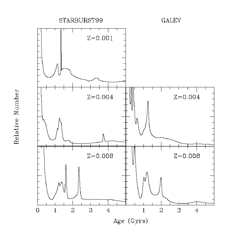
Figure 10.— Smoothed cluster age distributions derived with the Starburst and GALEV models (see text for details).

The answer to this question is more complicated than simply evaluating the number of clusters of a particular age. Our method for estimating ages can result in structure in the age distribution even if none is present. If the models traverse a large part of color space quickly and observational errors scatter clusters within the color space, an unrepresentative large fraction of the clusters may be close in color to the models that span a small age range. To determine how susceptible we are to this problem, we simulate our age measurements assuming an underlying smoothly exponentially declining cluster age function. We make no assumption here as to the cause of the exponential decline (whether it reflects a true decline in cluster formation or the disruption of clusters). We determine colors using both the S99 and GALEV models, add uncertainties drawn from our observational distribution, and then recover the age distribution using our technique. The resulting distributions often show some structure, as in the example from the GALEV Z = 0.004 simulations (Figure 11). To estimate whether the structure in these Monte-Carlo simulations is as strong as that in the data, we compare the areas under the peaks. We automate the measurement of the area and measure peak areas for both the data and 1000 simulations (for each of the model/metallicity combinations).

Figure 11.— Smoothed cluster age distributions derived with the GALEV models from Monte Carlo simulations (see text for details).

Our principal finding is that no peak is consistently significant across the range of models. While for certain metallicities, certain peaks are statistically signficant (probability of random occurrence $<0.05$), without knowing exactly which metallicity model is appropriate we are unable to conclude that any of the peaks are real. In short, both the precision of the colors and the systematic uncertainties inherent in the modeling preclude any conclusions regarding the fine structure of the cluster age distribution.

3.2. The Evolution of the Cluster System

Under the assumption that the cluster formation history is the same as that measured for the field stars, a comparison of the cluster age distribution and the field star formation history (Harris & Zaritsky, 2004) provides constraints on the evolution of the cluster system. Any variation in the number of clusters normalized by the corresponding star formation rate can be interpreted as the result of evolution of the cluster system. Various factors affect the cluster age distribution, some of which are observational, such as the loss from the sample of increasingly fainter or more diffuse clusters with age, and some of which are physical, such as the tidal disruption or evaporation of clusters. We begin by calculating the directly empirical quantity of the number of clusters of a given age divided by the number of stars formed at that time. We bin our clusters into the same age bins as used in the field star formation analysis. This calculation provides a star-formation normalized measure of the differential number of clusters as a function of time, which approaches $dN(t)/dt$ as the age bin size approaches zero. If the population of clusters formed as a fixed fraction of the field star formation and if clusters did not evolve, the ratio should be constant over time, which is evidently not the case (Figure 12).

Figure 12.— The number of clusters of age $t$ per number of stars formed over the equivalent time. The two panels show results from either Starburst99 (left) or the GALEV (right) models. Within each panel the symbols represent the results from either $Z=$ 0.001 (filled circles), 0.004 (open squares) or 0.008 (crosses). The line in the left panel represents a power-law distribution with $y\propto t^{-2.1}$.

The number of clusters currently existing as a function of lookback time, $dN(t)/dt$, is well-approximated by the power law function, $dN(t)/dt\propto t^{-2.1}$, shown in the Figure. The best fit slope value for $dN(t)/dt$ as measured using both the S99 and GALEV models of different metallicities ranges from $-1.73$ to $-2.18$, although four of the five slopes cluster between values of $-2.08$ and $-2.18$. In contrast to the details of the cluster age function described in §3.1, these results are nearly insensitive to the particular model used. To provide some intuition for how rapidly the number of clusters in the sample declines with age we note that for all the best-fit slopes more than half the clusters formed are lost less than 10 Myr after formation, and less than 1% of the clusters survive, where survive is simply defined as being part of the current sample, past an age of 1 Gyr.

The observed decline in the number of older clusters is due to a combination of selection and physical effects. Due to our selection of clusters as resolved stellar systems in which we observe stars well down the luminosity function, we do not expect strong age-dependent selection effects unless the structural properties of the clusters, such as the central surface density, evolve strongly with time. Our conclusion is similar to that reached by Boutloukos & Lamers (2003) for the Hodge (1987) SMC cluster sample. If this claim is correct, then the principal cause of the decline in the number of clusters is physical.

This interpretation is supported by the general agreement we find with previous studies of cluster disruption both in the SMC (Hunter et al., 2003; Boutloukos & Lamers, 2003) and other galaxies (Boutloukos & Lamers, 2003). To be specific, Boutloukos & Lamers (2003) have measured cluster disruption in a set of galaxies, including the SMC. In their modeling of the problem, they find that they can describe the slope of the cluster age function to be $(1-\alpha)/\gamma$, where $\alpha$ is the slope of the cluster initial mass function and $\gamma$ describes the power-law mass dependence of the disruption time, $t_{d}({M})\propto M^{\gamma}$. They find that on average $\gamma=0.57\pm 0.1$. From our slope of $-2.1$ in the SMC, we calculate that $\gamma=0.48$ for an assumed $\alpha=2$, which is the value of $\alpha$ also assumed by Boutloukos & Lamers (2003). Alternatively, we could adopt the mean value of $\gamma$ presented by Boutloukos & Lamers (2003) and calculate $\alpha=2.2$, in agreement with the typical cluster initial mass function found in other galaxies (Zhang & Fall, 1999; Whitmore et al., 1999; Bik et al., 2003) and within the range of 2 to 2.4 found for the LMC and SMC by Hunter et al. (2003).

One aspect in which we do identify a disagreement with previous studies is in the time at which disruption dominates over fading for the SMC cluster population. Boutloukos & Lamers (2003), using data from Hodge (1987), identify a bend in $dN(t)/dt$, at $\log{t}=8.8$, that is associated with this transition. We find no unambiguous flattening of $dN(t)/dt$ at that, or any other, time. However, due to uncertainties, we cannot rule out a flattening at $\log{(t)}<8.5$ for the S99 models, or for $\log(t)<7$ in any of our models. The latter could correspond to a disruption timescale that agrees with what Boutloukos & Lamers (2003) find for other galaxies. As discussed in §2.1, we have a strong bias against finding young clusters, and therefore the $dN(t)/dt$ function is likely to be even steeper at young ages than what we have plotted in Figure 12. The lack of a strong flattening signature and the uncertainty posed by incompleteness preclude us from placing strong constraints on any flattening at $\log(t)<8.5$.

3.3. Investigating the Age Gap

The field star formation history (Harris & Zaritsky, 2004) shows two pronounced peaks at about 0.4 and 2.5 Gyr. As we described above, such peaks are seen in the cluster age distribution for certain choices of model type and metallicity. While we cannot confirm that these peaks exist in the cluster age function, neither can we exclude the possibility. Our inability to resolve peaks is a consequence of the low precision of our age estimates. However, another interesting feature of cluster age functions, particularly in the LMC, is the presence of an “age gap”. A similar lull in star formation is observed in the global star formation of the SMC (Harris & Zaritsky, 2004). Can we reach any conclusion about cluster formation over the timescale of this lull (from 3 to 8 Gyr)?

In Figure 13 we show the distribution for cluster ages between 1 and 15 Gyr (there are no clusters at measured ages $>$ 15 Gyr) for both the S99 and GALEV models with Z = 0.004. The distributions qualitatively show an initial, older epoch of clusters and a recent epoch of cluster formation (starting within 3 Gyr of the current time), with a relatively quiet time between. The quantitative details, however, are quite different between the models. First, the oldest clusters in the S99 models are only 8 Gyr old. If this is correct, or if we are incomplete in older clusters, then this peak would correspond to the $\sim$ 8 Gyr clusters identified by Rich et al. (2000). On the other hand, if there is a systematic error in the entire scale of ages, and the older peak corresponds to the oldest LMC clusters which are $>$ 10 Gyr old, then perhaps the intermediate peak (currently located at $\sim$ 4 Gyr) corresponds to the 8 Gyr clusters. Curiously, the GALEV models also show an intermediate age peak (at $\sim$ 6 Gyr), which could correspond to the hypothesized 8 Gyr population, and these models do identify a truly old, $>$ 10 Gyr, population of SMC clusters. In both sets of models, the SMC appears to have had an initial cluster formation epoch followed by relatively little cluster formation, with the possible exception of an intermediate age peak, punctuated with a recent ($<3$ Gyr old) episode of cluster formation that is at least as strong as the original epoch.

Figure 13.— The number of clusters of age $t$. The two panels include the results from either Starburst99 (left) or the GALEV models (right) for Z = 0.004.

A different picture of the cluster history is presented if we remove the effect of cluster dissolution. In Figure 14 we have presented the entire cluster age distribution, but we have normalized by the $t^{-2.1}$ dependence of the cluster number. From this Figure it is evident that the initial episode of cluster formation dominates the rate of cluster formation in the SMC. This Figure rests on the assumption that the cluster destruction function remains constant in time. From either model, one can conclude that the initial flurry of cluster formation (at 11 to 14 Gyr in the Galev models or 6-8 Gyr in the S99 models) did subside, but whether there is an age gap (as seen for 6 to 11 Gyr in the Galev models) or rather a continuous low level of cluster formation (as seen for $t\leq 5$ Gyr in the S99 models) depends on the model. The more dramatic impression of an age gap presented in Figure 13 is due to the fact that the clusters formed in the most recent episode of cluster formation have had insufficient time to dissolve.

Figure 14.— The number of clusters of age $t$ normalized by the expected dissolution function, $\Delta N(t)\propto t^{-2.1}$. The two panels include the results from either Starburst99 (left) or the GALEV models (right) for Z = 0.004.

3.4. Spatial Distribution

The distribution of clusters of different ages may constrain models of how clusters formed or were destroyed. van den Bergh (1991) shows that among his sample of SMC clusters the young clusters lie along the SMC “bar”, while the older clusters form more of halo. Although the dynamical reality of the bar has been questioned (Zaritsky et al., 2000), the distribution of younger and older stars in the SMC follows a similar pattern in that the younger stars are preferentially found along the north-east/south-west axis while the older stars lie in a spheroidal distribution. In Figure 15 we plot the distribution of clusters divided into a young (age $<$ 3.5 Gyr) and old (age $>$ 3.5 Gyr) samples for S99 and GALEV models with Z = 0.004. The characteristics of the distributions, centroid, ellipticity, and position angle are different, particularly for the S99 model, which has more clusters in the older bin. For example, the right ascension centroids of the young and old population are highly discrepant ($0.942\pm 0.015$ and $0.860\pm 0.028$ in decimal hours, respectively, which corresponds to a difference that is different than zero at more than 2.6$\sigma$ significance), while the declination centroids are consistent ($-72.853\pm 0.07$ and$-72.791\pm 0.11$ in decimal degrees).

Figure 15.— The distribution of young (age $<$ 3.5 Gyr) and old (age $>$ 3.5 Gyr) clusters using ages determined with either the S99 or GALEV models (with Z = 0.004).

Because of the poor temporal resolution of our age measurements, we are unable to confidently explore other age bins, but such a study with higher precision ages may help resolve the origin of the gas that is hypothesized to have infallen (Zaritsky & Harris, 2004) and the disturbed morphology of the young stars (Zaritsky et al., 2000). Correlations among spatial properties and marginally detected age peaks would also increase the confidence of any identified structure in the cluster age function.

4. Conclusions

We use the images from the Magellanic Clouds Photometric Survey (Zaritsky et al., 2002) to measure integrated $U,B,V$ and $I$ colors for a sample of 195 stellar clusters with measured structural parameters (Hill & Zaritsky, 2003). We estimate cluster ages for 195 of these using those colors and models of simple stellar populations. We conclude that:

1) Although peaks are visible in the cluster age distribution, the location of these varies sensitively with the choice of metallicity and model type, and similar peaks can arise by chance.

2) We find that the rate of cluster number evolution for clusters of age $t$, after normalizing by the number of stars formed at age $t$, is given by $dN(t)/dt\propto t^{-2.1}$ .

3) If this decline in the number of clusters with age is attributed primarily to physical destruction of the clusters, we calculate that the disruption timescale at a fixed mass is $t_{d}(M)\propto M^{0.48}$ for a cluster initial mass function $N(M)\propto M^{-2}$. This result is in agreement with the average value measured in a set of nearby galaxies, $M^{0.57\pm 0.1}$ (Boutloukos & Lamers, 2003). Alternatively, when we adopt the average value for the disruption timescale from Boutloukos & Lamers (2003), we calculate that the initial mass function $N(M)\propto M^{-2.2}$. These values are consistent with results from previous studies on other galaxies and the SMC. The agreement implies that cluster dissolution is highly effective and relatively independent of the host galaxy. Only 1% of clusters formed in the SMC will survive beyond 1 Gyr. This makes comparison of properties between clusters in the SMC and other systems, like the Milky Way, very difficult unless ages are known for all the clusters.

4) There is no evidence of a significant age gap in the SMC, although the dominance of the initial epoch of cluster formation in conjunction with the rapid dissolution of clusters produces an observed cluster age function that appears to have a formation lull at intermediate ages.

5) The spatial distribution of the younger and older clusters is statistically different, and supports the hypothesis of a significant accretion or merger event at around 3 to 5 Gyr.

The principal shortcoming of this study is the lack of precision in our age measurements that are both the result of photometric integrated colors that are susceptible to large scatter, some of which may be inherent to the cluster population, and cluster models that do not predict consistent colors for a given age, partly due to the lack of metallicity constraints. This problem of age and metallicity degeneracy was also examined by de Grijs et al. (2003) in their study of the systematic uncertainties in cluster age determinations in more distant galaxies using aperture photometry and stellar population models. The Magellanic Cloud clusters are particularly valuable in addressing these issues because ages from stellar color-magnitude diagrams can be compared to those of integrated colors (§2.3). The current limitation is the small number of cluster color-magnitude diagrams currently available. To further address the question of systematics, our study can provide guidance as to which clusters to target for more precise age measurements. Such observations benefit both the study of the Magellanic Clouds and of more distant systems.

5. Acknowledgments

We thank the anonymous referee for a careful reading of the manuscript. MR acknowledges financial support from the Baird Foundation and scholarships from the University of Arizona. DZ acknowledges financial support from National Science Foundation CAREER grant AST-9733111, AST-0307482, and a fellowship from the David and Lucile Packard Foundation.

References

- Anders and Fritze-v. Alvensleben (2003) Anders, P. & Fritze-v. Alvensleben, U. 2003, A&A, 401, 1063
- Baird et al. (1974) Baird, S., Flower, P., Hodge, P., and Szkody, P. 1974, AJ, 79, 1365
- Bica & Schmitt (1995) Bica, E.L.D. & Schmitt, H.R. 1995, ApJS, 101, 41
- Bica & Dutra (2000) Bica, E. & Dutra, C.M. 2000, AJ, 119, 1214
- Bik et al. (2003) Bik, A., Lamers, H.J.G.L.M., Bastian, N., Panagia, N., Romaniello, M. 2003, A&A, 397, 473
- Boutloukos & Lamers (2003) Boutloukos, S.G., & Lamers, H.J.G.L.M. 2003, MNRAS, 338, 717
- Brück (1976) Brück, M.T. 1976, Occ. Rep. R. Obs. Edinburgh, 1, 1
- Da Costa (1991) Da Costa, G. S. 1991, in Proc. IAU Symp. 148, The Magellanic Clouds, Haynes R,. Milne, D., eds (Kluwer, Dordrecht), p. 183
- Da Costa & Hatzidimitriou (1998) Da Costa, G. S., & Hatzidimitriou, D. 1998, AJ, 115, 1934
- de Freitas Pacheco et al. (1998) de Freitas Pacheco, J.A., Barbuy, B., & Idiart, T. 1998, A&A, 332, 19
- de Grijs et al. (2003) de Grijs, R. et al. 2003, MNRAS, 342, 259
- de Oliveira et al. (2000) de Oliveira, M.R., Dutra, C.M., Bica, E., & Dottori, H. 2000, A&AS, 146, 57
- Dopita et al. (1985) Dopita, M. A., Lawrence, C. J., Ford, H. C., & Webster, B.L. 1985, ApJ, 296, 390
- Harris & Zaritsky (2004) Harris, J., & Zaritsky, D. 2004, AJ, 127, 1531
- Hill & Zaritsky (2003) Hill, A. & Zaritsky, D. 2003, AJ, submitted
- Hodge (1961) Hodge, P. W. 1961, ApJ, 133, 413
- Hodge (1985) Hodge, P. W. 1985, PASP, 97, 530
- Hodge (1986) Hodge, P. W. 1986, PASP, 98, 1113
- Hodge (1987) Hodge, P. 1987, PASP, 99, 742
- Hodge & Wright (1974) Hodge, P.W., & Wright, F.W. 1974, AJ, 79, 858
- Holtzman et al. (1992) Holtzman, J.A. et al. 1992, AJ, 103, 691
- Hunter et al. (2003) Hunter, D.A., Elmegreen, B.G., Dupuy, T.J., & Mortonson, M. 2003, AJ, 126, 1836
- Jensen et al. (1988) Jensen, J., Mould, J. & Reid, N. 1988, ApJS, 67, 77
- Kron (1956) Kron, G.E. 1956, PASP, 68, 125
- Leitherer et al. (1999) Leitherer et al. 1999, ApJS, 123, 3
- Lindsay (1958) Lindsay, E.M. 1958, MNRAS, 118, 172
- Mighell et al. (1998) Mighell, K.J., Sarajedini, A., & French, R.S. 1998, AJ, 116, 2395
- Pagel & Tautvais̆ienė (1998) Pagel, B.E.J., & Tautvais̆ienė, G. 1998, MNRAS, 299, 535
- Piatti et al. (2001) Piatti, A.E., Santos, João, F.C., Clariá, J.J., Bica, E., Sarajedini, A., & Geisler, D. 2001, MNRAS, 325, 792
- Pietrzyński et al. (1999) Pietrzyński, G. & Udalski, A. 1999, AcA, 49, 157
- Pietrzyński et al. (1998) Pietrzyński, G., Udalski, A., Kubiak, M., Szymanski, M., Wozniak, P., & Zebrun, K. 1998, AcA, 48, 175
- Rich et al. (2000) Rich, R.M., Shara, M., Fall, S.M., and Zurek, D. 2000, AJ, 119,197
- Rich et al. (2001) Rich, R.M., Shara, M., and Zurek, D. 2001, AJ, 122, 842
- Schild (1977) Schild, R. E. 1977, AJ, 82, 337
- van den Bergh (1991) van den Bergh, S. 1991, ApJ, 369, 1
- van den Bergh (1981) van den Bergh, S. 1981, A&AS, 46, 79
- Whitmore et al. (1993) Whitmore, B.C., Schweizer, F., Leitherer, C., Borne, K., & Robert, C. 1993, AJ, 106, 1354
- Whitmore et al. (1999) Whitmore, B.C., Zhang, Q., Leitherer, C., Fall S.M., Schweizer, F., Miller, B.W. 1999, AJ, 118, 1551
- Zaritsky (1999) Zaritsky, D. 1999, AJ, 118, 2824
- Zaritsky & Harris (2004) Zaritsky, D., & Harris, J. 2004, ApJ, 604, 167
- Zaritsky et al. (2000) Zaritsky, D., Harris, J., Grebel, E.K., & Thompson, I.B. 2000, ApJ, 534, L53
- Zaritsky et al. (2002) Zaritsky, D., Harris, J., Thompson, I.B., Grebel, E.K., & Massey, P. 2002, AJ, 123, 855
- Zaritsky et al. (1996) Zaritsky, D., Shectman, S.A., & Bredthauer, G. 1996, PASP, 108, 104
- Zhang & Fall (1999) Zhang, Q. & Fall, S.M 1999, ApJ, 527, L81