A wavelet add-on code for
new-generation $N$-body simulations and data de-noising
(JOFILUREN)

Abstract

Wavelets are a new and powerful mathematical tool, whose most celebrated applications are data compression and de-noising. In Paper I (Romeo, Horellou & Bergh 2003), we have shown that wavelets can be used for removing noise efficiently from cosmological, galaxy and plasma $N$-body simulations. The expected two-orders-of-magnitude higher performance means, in terms of the well-known Moore’s law, an advance of more than one decade in the future. In this paper, we describe a wavelet add-on code designed for such an application. Our code can be included in common grid-based $N$-body codes, is written in Fortran, is portable and available on request from the first author. The code can also be applied for removing noise from standard data, such as signals and images.

1 INTRODUCTION

In $N$-body simulations the number of particles $N$ cannot generally be set equal to the number of bodies of the real system, but is dictated by the available computer power. A simulation with, say, ten times more particles demands at least one order of magnitude more computational time, memory and storage. Because of such a limitation, $N$ is generally several orders of magnitude smaller than required. A small $N$ means that the statistical fluctuations of particle positions and velocities are artificially enhanced, and so are collisional effects. This is dangerous because collisions affect the ability of resonances to damp or amplify perturbations, which in turn affects the formation of structures and the dynamical evolution of the model. Thus an effective method of noise reduction is required.

The standard way to reduce noise in $N$-body simulations is to soften the interparticle force at short distances, either directly or using finite-sized particles (e.g., Romeo 1994, 1997, 1998a, b; Dehnen 2001; see also Byrd 1995). On the other hand, softening reduces noise only in part. The initial conditions imposed on particle positions and velocities are also relevant. Basically, noise can be suppressed at the beginning of the simulation by sampling phase space regularly (quiet starts), rather than randomly (noisy starts), consistent with the distribution function of the model (e.g., Dawson 1983; Birdsall & Langdon 1991; Knebe, Green & Binney 2001). Even so, noise will develop during the simulation. In fact, quiet starts impose an initial order on the model. But the model will react to such a state of low entropy and follow the natural tendency of physical systems towards thermalization. The development of noise is mediated by instabilities, which amplify and randomize the initial correlations arising from the discrete regular sampling of phase space.

The effects of noise are subtle and not yet fully understood. Today, half a century after the first $N$-body simulations, there is still an intense debate. Noise is a crucial issue for simulations of structure formation in the early Universe (e.g., Splinter et al. 1998; Hamana, Yoshida & Suto 2002; Power et al. 2003; Binney 2004; Diemand et al. 2004; Sylos Labini, Baertschiger & Joyce 2004), and for galaxy simulations (e.g., Pfenniger 1993; Pfenniger & Friedli 1993; Weinberg & Katz 2002; O’Neill & Dubinski 2003; Valenzuela & Klypin 2003). Noise is an important issue not only for cosmology and astrophysics but also for plasma and accelerator physics, where simulations are used for technological applications such as fusion and charged particle beams (e.g., Dawson 1983; Birdsall & Langdon 1991; Arter 1995; Kandrup 2003). The noise problem is acute and awaits solution.

Wavelets are the state-of-the-art technique used for noise reduction in digital signal/image processing (see, e.g., Mallat 1998; Bergh, Ekstedt & Lindberg 1999; for traditional techniques such as data averaging or Wiener filtering see, e.g., Gonzalez & Woods 2002). Wavelets have an intrinsic ability to compress the signal into few large coefficients, so that noise can be removed with a proper thresholding. Being intrinsic, their ability is independent of general properties of the data such as the number of dimensions or the presence of symmetries. Wavelet de-noising is very effective: it outperforms traditional techniques of noise reduction and the algorithm is even faster than the fast Fourier transform. The second aspect is especially important for our application since speed is a primary factor in $N$-body simulations. We recommend the following literature: for the continuous and fast wavelet transforms see Addison (2002) and Goedecker (1998), respectively; for physical applications see again Goedecker (1998) and the beautiful book by van den Berg (2004).

In Paper I, we have pioneered the first application of wavelet de-noising to $N$-body simulations. Our method has been subjected to several hard tests. The conclusion is that it can make the simulation equivalent to a simulation with two orders of magnitude more particles. The implications are clear.

In the present paper, we show that our method even allows controlling the effectiveness of de-noising: the simulation can be made equivalent to a simulation with $\Gamma$ times more particles, where $\Gamma$ is assigned by the simulator beforehand. Such a degree of freedom can be exploited for understanding the effects of noise more thoroughly. Besides, we describe the code that implements our method. It is an add-on code, and as such is meant to be included in the simulator’s $N$-body code. This is simple if the $N$-body code is of particle-mesh type. Our code can also be used by itself for de-noising standard data, such as signals and images. It is written in Fortran, is portable and available on request from the first author. Last but not least, we have the ambition to provide a reader-friendly and self-contained discussion of wavelet de-noising, from the basics to the most advanced aspects of our problem. For further reading see Paper I and the literature already recommended.

The rest of our paper is organized as follows. Wavelets and wavelet applications are overviewed in Sects 2 and 3, respectively. Sect. 3.2 not only discusses the basics of de-noising, but also explains the steps of the de-noising algorithm in our code. These are then discussed in detail in Sect. 4. After such a tour of the code, we explore advanced de-noising in Sect. 5. There we learn how to control the effectiveness of de-noising, and how this part of the method is implemented in the code; besides, we discuss further aspects of the problem. Practical points concerning the use of the code are discussed in Sect. 6. Finally, the conclusions are drawn in Sect. 7.

2 BASICS OF WAVELETS

2.1 The fundamental property of wavelets

Data such as signals, images and those arising from the numerical solution to physical problems generally enclose information on various scales. In order to extract such information, we should be able to separate small-scale features from large-scale features and to understand their contributions to the overall structure of the data. The classical technique used for this purpose is the Fourier transform, which encodes the original time/space information into frequency content of the data, the frequency being roughly the inverse of the relevant scale. But the Fourier transform runs into a serious difficulty: it loses all information about the time/space localization of a given frequency component. This is nothing but the consequence of the Heisenberg uncertainty principle in the context of data processing.

The traditional way to overcome this difficulty is to localize the complex sinusoid of the transform multiplying it by a window function, a Gaussian for example, which is then translated across the data. For a window of given shape, its width determines not only the time/space resolution but also the frequency resolution, again as a consequence of the Heisenberg uncertainty principle. A narrow window gives a good time/space resolution but a bad frequency resolution, and vice versa for a wide window. So how should we choose the width of the window? If we choose it comparable to the smallest scale of interest, the time/space resolution of course matches the data, but the frequency localization is too poor to resolve the low frequencies characterizing large-scale features. And if we choose a wider window so as to have a finer frequency resolution, the time/space resolution gets too coarse to analyse small-scale features. Thus even the windowed Fourier transform runs into a difficulty: it has a fixed time/space-frequency resolution [constant bandwidth, in the language of data processing; cf. Paper I, fig. 1 (left-hand panel)].

Wavelets are a multi-scale method that overcomes this difficulty. Their fundamental property is to provide an adaptive time/space-frequency resolution, in the sense that the uncertainty in frequency is proportional to the frequency itself [constant relative bandwidth, in the language of data processing; cf. Paper I, fig. 1 (right-hand panel)]. In other words, this means that small-scale features of the data are analysed with fine resolution in time/space and coarse resolution in frequency, as is natural, and vice versa for large-scale features.

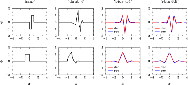
Figure 1: Various wavelets $\psi(x)$ and scaling functions $\phi(x)$. The wavelets ‘haar’ and ‘daub 4’ are orthogonal. The wavelet pairs ‘bior 4.4’ and ‘rbio 6.8’ are bi-orthogonal and also quasi-orthogonal, hence for each of them the decomposition (‘dec’) and reconstruction (‘rec’) wavelets are distinct but similar. Analogous considerations apply to the scaling functions.

2.2 Wavelet transform

In order to provide an adaptive time/space-frequency resolution, the wavelet analysis involves localized wave-like functions, which are contracted or dilated over the relevant range of scales and translated across the data. On the other hand, there are several ways to carry out the analysis, depending on whether the data are continuous or discrete; and, in the discrete case, depending on technical factors. Here we present the wavelet transform that is most appropriate for our application, which is also the one most commonly used for compressing and de-noising discrete data.

The contributions of small-scale and large-scale features are singled out with an iterative procedure. The first step consists of separating the smallest-scale features from the others. It is done by passing the data through a high-pass filter and a complementary low-pass filter. These filters are the discrete counterparts of the analysing functions of the transform, the wavelet $\psi(x)$ and the scaling function $\phi(x)$ respectively, and are constructed with a mathematical technique known as multi-resolution analysis. Filtering produces redundant information, since each set of filtered data has the same size as the original data. Redundancy is avoided by rejecting every other point of the filtered data. It is well known that down-sampling produces aliasing in the context of the Fourier transform, but the filters of the wavelet transform are constructed in such a way as to eliminate it. The second step consists of separating the features that appear on a scale twice as large as in the first step. It is done by regarding the low-pass filtered and down-sampled data as new input data, and by analysing them as in the first step. The procedure continues until the largest-scale features are also separated. In summary, the wavelet transform decomposes the original data into a coarse approximation and a sequence of finer and finer details, keeping the total size of the data constant (cf. Paper I, fig. 2). We can draw an analogy with art and say that the approximation gives an ‘Impressionist’ view of the data!

The original data can be reconstructed with the inverse wavelet transform. The coarsest approximation and detail are up-sampled, filtered and added. Here up-sampling means inserting zeros between the data points, and the filters are closely related to the decomposition filters so as to eliminate aliasing. The output is a finer approximation, which is then combined with the corresponding finer detail as above, and the procedure is iterated. In practice, the wavelet synthesis is carried out for reconstructing data that have been processed in wavelet domain, such as in data compression and de-noising.

The great success of the wavelet transform arises not only from its adaptive time/space-frequency resolution, but also from its speed: it is even faster than the fast Fourier transform. Given data of size $N_{\mathrm{d}}=2^{J}$ ($J$ positive integer) and filters of effective size $2M$, the fast wavelet transform is computed with $4MN_{\mathrm{d}}$ arithmetic operations, where $M$ is a positive integer independent of $N_{\mathrm{d}}$ and typically smaller than ten. In contrast, the fast Fourier transform has complexity $2N_{\mathrm{d}}\log_{2}N_{\mathrm{d}}$. Note that such an efficiency follows directly from the non-redundancy of the transform. Similar considerations apply to the inverse fast wavelet transform.

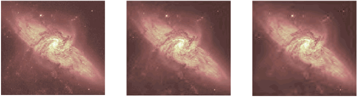
Figure 2: The original image of the spiral galaxy pair NGC 3314 (left) is compressed by a factor of 200 with only 0.29% loss of information (middle) and by a factor of 500 with only 0.52% loss of information (right). The original image is from Hubble Heritage, courtesy of NASA and STScI.

2.3 Wavelet properties

In contrast to classical transforms, where the analysing functions belong to a single class and are defined analytically, there are dozens of wavelet families and their members are generally defined numerically through the associated filters. Why do we have so many choices? Because, even though the fast wavelet transform has an adaptive time/space-frequency resolution, there are various ways to optimize the trade-off between time/space and frequency localizations, and different conditions can be imposed. In other words, wavelets are not all equivalent in applications and, if we want to choose the optimal wavelet for a given problem, we must understand their properties well. The properties of the scaling functions are determined by those of the wavelets, but are themselves less relevant. The wavelet properties are: size of support, symmetry, number of vanishing moments, regularity and (bi-)orthogonality.

Size of support. The support of a wavelet is the interval where the wavelet is non-zero. Its size determines not only the time/space localization of the wavelet, but also the speed of the transform.

Symmetry. Symmetry also influences the quality of time/space localization. For example, an asymmetric wavelet can be regarded as giving a location with asymmetric error bars.

Number of vanishing moments. A wavelet $\psi(x)$ has $n$ vanishing moments when

$$\int_{-\infty}^{+\infty}x^{\nu}\psi(x)\mathrm{d}x=0\mbox{\ \ \ \ for\ \ }\nu=0,1,\ldots,n-1\,;$$ (1)

where $x$ denotes time or space. In particular, all ‘normal’ wavelets have zero mean ($n=1$) since, under rather general assumptions, this is related to the admissibility condition for the existence of the inverse transform. The number of vanishing moments affects the frequency localization. In fact, the Fourier transform of a wavelet with $n$ vanishing moments peaks at a characteristic frequency and decays as $k^{n}$ towards the origin, where $k$ denotes frequency.

Regularity. Regularity also affects the frequency localization. In fact, the Fourier transform of a wavelet that is continuous together with its first $n-1$ derivatives decays as $k^{-(n+1)}$ towards infinity.

(Bi-)Orthogonality. The orthogonality property concerns the set of wavelets defining the transform, that is the set of scaled and translated versions of the basic wavelet. It means that such wavelets form an orthogonal basis. The alternative bi-orthogonality property means that the decomposition and reconstruction wavelets form two distinct bases, which are mutually orthogonal. Note that (bi-)orthogonality is intimately related to the non-redundancy of the transform.

It follows that a good time/space localization requires a small support and high symmetry, and a good frequency localization requires many vanishing moments and high regularity. A small support is also needed for a faster transform. On the other hand, the wavelet properties are interrelated. A small support implies relatively few vanishing moments and low regularity. In addition, orthogonality implies asymmetry, except for the simplest wavelet. Bi-orthogonality weakens the coupling between the properties of the decomposition and reconstruction wavelets, and allows perfect symmetry. This means that the requirements above cannot be satisfied equally well. In order to choose a good wavelet, we should then know their relative importance, which depends on the application.

2.4 What do wavelets look like?

Let us now illustrate what wavelets and scaling functions look like. (Recall that the scaling functions are the continuous counterparts of the low-pass filters of the fast wavelet transform and its inverse; see Sect. 2.2, and also Sect. 2.3.) Fig. 1 shows various representatives. The wavelets ‘haar’ and ‘daub 4’ belong to the family of Daubechies wavelets, and are simple (see Daubechies 1992; here we use the same names as in the code). These wavelets are orthogonal; and they have few vanishing moments, small support, low regularity and no symmetry (‘haar’ is an exception). The wavelet pairs ‘bior 4.4’ and ‘rbio 6.8’ belong to the family of bi-orthogonal spline wavelets and to its reverse, respectively, and are more advanced (see Daubechies 1992; here we use the same names as in the code). Such wavelet pairs are not only bi-orthogonal but also quasi-orthogonal: for each pair the decomposition and reconstruction wavelets are distinct but similar. In addition, they have more vanishing moments, larger support, higher regularity and perfect symmetry.

3 BASICS OF WAVELET APPLICATIONS

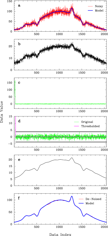
Figure 3: De-noising in action. a: data with Poissonian noise and the perfectly non-noisy model data. b: pre-processed data. c: wavelet coefficients computed by fast wavelet transforming, after the choice of the wavelet; note that there are few large wavelet coefficients and many small wavelet coefficients. d: original and thresholded wavelet coefficients; the threshold is also shown. e: data computed by inverse fast wavelet transforming. f: de-noised data computed by post-processing vs. the model data. The signal-to-noise ratio is $\mathit{SNR}\simeq 8.8$ in the noisy data and $\mathit{SNR}\simeq 73.9$ in the de-noised data, hence the de-noising factor is $\mathit{DF}\simeq 8.4$. (For more information see the text.)

3.1 Data compression

The adaptive time/space-frequency resolution and the non-redundancy of the fast wavelet transform have an important implication: given regular data, most information present in them gets concentrated into few large wavelet coefficients. In practice, this means that we can set all the other coefficients to zero and get back data almost identical to the original ones. This is the idea behind data compression.

The compression ability can be quantified by the compression factor $\mathit{CF}$ and the loss of information $\mathit{LI}$, defined as:

$$\mathit{CF}=\frac{N_{W}}{n_{w}}\,,$$ (2)

$$\mathit{LI}\,[\%]=100\left(1-\frac{{\displaystyle\sum}\,w_{i}^{2}}{{\displaystyle\sum}\,W_{i}^{2}}\right)\,,$$ (3)

where $N_{W}$ is the number of wavelet coefficients $W_{i}$ (and is equal to the number of data points $N_{\mathrm{d}}$), and $n_{w}$ is the number of wavelet coefficients $w_{i}$ that are not set to zero. Clearly, there are also visual criteria for judging the quality of the compressed data.

The most important requirement for a good compression ability (large $\mathit{CF}$ and small $\mathit{LI}$) is that the decomposition wavelet should have many vanishing moments, and the basic reason is the following. A wavelet with $n$ vanishing moments is insensitive to polynomials of degree $n-1$. Regular data behave approximately as such polynomials in a neighbourhood of a given point. Hence the wavelet only feels the deviation from such behaviour, which decreases with $n$. Thus a large $n$ means that the detail coefficients tend to be small and this implies a potentially good compression ability. On the other hand, a good compression ability is guaranteed only if the decomposition wavelet has a sufficiently small support. Basically, the analysis should be local enough otherwise the deviation from polynomial behaviour of the data becomes significant. (For a more explicit condition see Sect. 4.2.) Lastly, high regularity and symmetry are mainly needed by the reconstruction wavelet for a good quality of the compressed data. The conclusion is that bi-orthogonal wavelets represent the best alternative for satisfying the requirements above.

Let us then consider a beautiful image of disc galaxies and choose an appropriate wavelet pair, ‘rbio 2.8’, which belongs to the family of reverse bi-orthogonal spline wavelets (see Daubechies 1992; here we use the same name as in the code). Fig. 2 illustrates the example eloquently.

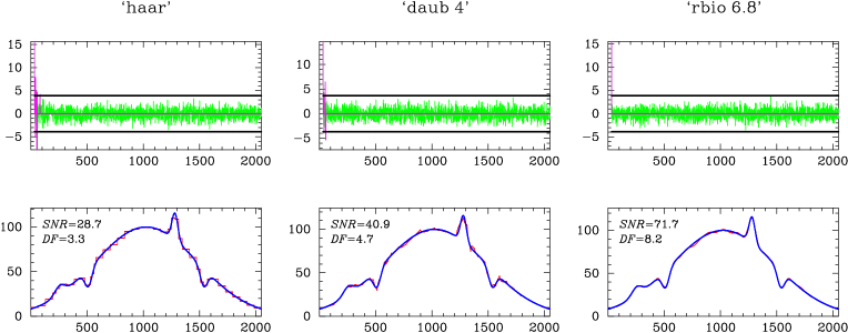
Figure 4: Original and thresholded wavelet coefficients (top), and de-noised data vs. the model data (bottom) for various choices of the wavelet. Also specified are the signal-to-noise ratio $\mathit{SNR}$ in the de-noised data and the de-noising factor $\mathit{DF}$. The reference case illustrated in Fig. 3 corresponds to ‘bior 4.4’.

3.2 De-noising: data and simulations

The compression ability of the fast wavelet transform has a further important implication: given noisy data, the underlying regular part gets mostly concentrated into few large wavelet coefficients, whereas noise is mostly mapped into many small wavelet coefficients. In practice, this means that, if we identify a correct threshold, then we can set all the small coefficients to zero and get back data almost decontaminated from noise. This is the idea behind data de-noising: a rigorous way to compress noisy data. In this section, we go on discussing the basics of de-noising. A more detailed discussion is given in Sect. 4. The identification of a correct threshold, which is crucial to the whole process of de-noising, is discussed in Sect. 4.4.

Let us now illustrate the basics of de-noising in a concrete case (cf. Fig. 3). Fig. 3a shows data with Poissonian noise and the perfectly non-noisy model data. This type of noise is characterized by a multivariate Poissonian probability distribution, and hence the local standard deviation of the data is equal to the square root of their local mean: $\sigma_{\mathrm{loc}}=\sqrt{\mu_{\mathrm{loc}}}$ (see, e.g., Bevington & Robinson 1992). Poissonian noise occurs in all experiments and observations where the data represent ‘counts’ in a set of bins. Fig. 3b shows that the noisy data are pre-processed so as to transform Poissonian noise into Gaussian white noise, where ‘white’ means that it is equally significant on all scales (constant power spectrum). This type of noise is well known for its mathematical tractability (see, e.g., Gonzalez & Woods 2002). In fact, the reason for pre-processing the data is that Gaussian white noise is convenient for identifying a correct threshold. Figs 3c–f show the remaining route after the choice of the wavelet: fast wavelet transforming (Fig. 3c); thresholding the wavelet coefficients, which is the heart of de-noising (Fig. 3d); inverse fast wavelet transforming (Fig. 3e); and, finally, post-processing the data, which is needed after the initial pre-processing (Fig. 3f). The de-noised data are shown vs. the model data.

As in Fig. 3 the model data are known, the de-noising ability can be quantified by the signal-to-noise ratio $\mathit{SNR}$ and the de-noising factor $\mathit{DF}$, defined as:

$$\mathit{SNR}=\left[\frac{{\displaystyle\sum}\,X_{i}^{2}}{{\displaystyle\sum}\,(Y_{i}-X_{i})^{2}}\right]^{1/2}\,,$$ (4)

$$\mathit{DF}=\frac{(\mathit{SNR})_{\mathrm{de}}}{(\mathit{SNR})_{\mathrm{no}}}\,,$$ (5)

where $X_{i}$ are the model data and $Y_{i}$ are either the noisy data (‘no’) or the de-noised data (‘de’). In addition, $(\mathit{SNR})_{\mathrm{de}}$ means the inverse of an appropriately defined estimation error. Clearly, there are also visual criteria for judging the quality of the de-noised data. Fig. 3 illustrates the improvement produced by de-noising expressively. In general, the model data are not known so the de-noising ability and the quality of the de-noised data are difficult to estimate.

2-D or 3-D data de-noising is similar to the 1-D case. The differences are discussed together with other details of de-noising (see Sect. 4).

How does de-noising work for N-body simulations? The de-noising method discussed here applies to discrete data so it is natural to consider grid-based $N$-body simulations. Such simulations use a grid for tabulating the particle density, and for computing the potential and the field (see, e.g., Hockney & Eastwood 1988). The number of particles $n$ in each cell shows fluctuations $|\delta n|/\langle n\rangle\sim\langle n\rangle^{-1/2}$ with respect to an average $\langle n\rangle$. This means that the particle distribution is polluted by noise that is basically Poissonian, whereas the noise induced in the potential and in the field is of a more complex nature. Using such a method we can thus de-noise the particle distribution at each timestep and make the simulation equivalent to a simulation with many more particles. This is the idea behind our application (cf. Paper I).

4 TOUR OF THE CODE

As we have explained in Sect. 3.2, de-noising standard data and $N$-body simulations consists of the following processes: pre-processing of the data, choice of the wavelet, fast wavelet transform, thresholding of the wavelet coefficients, inverse fast wavelet transform and post-processing of the data. These are also the steps of the de-noising algorithm in our code. In this section, we discuss them in detail. Advanced aspects of de-noising are discussed in Sect. 5.

4.1 Pre-processing of the data

The data should be pre-processed if they are contaminated by Poissonian noise. The Poissonian data $Y_{\mathrm{P}}$ are transformed into data $Y_{\mathrm{G}}$ with (additive) Gaussian white noise of standard deviation $\sigma_{\mathrm{G}}=1$:

$$Y_{\mathrm{G}}=2\,\sqrt{Y_{\mathrm{P}}+{\textstyle\frac{3}{8}}}$$ (6)

(Anscombe 1948), which can then be de-noised as discussed in Sects 4.2–4.5. The Anscombe transformation has the remarkable property to help achieving normalization, variance stabilization and additivity (see Stuart & Ord 1991). On the other hand, it has a tendency to fail locally where the data have small values or large variations (e.g., Kolaczyk 1997; see also Starck, Murtagh & Bijaoui 1998). On the whole, such an ingenious method produces very good results if the data are post-processed appropriately (see Sect. 4.6).

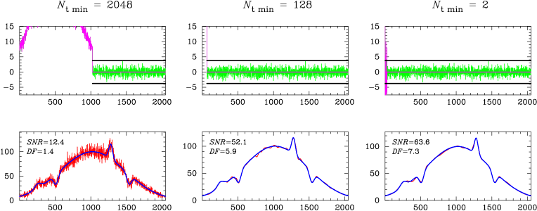
Figure 5: Original and thresholded wavelet coefficients (top), and de-noised data vs. the model data (bottom) for various values of the parameter $N_{\mathrm{t\,min}}$ defined in the text. Also specified are the signal-to-noise ratio $\mathit{SNR}$ in the de-noised data and the de-noising factor $\mathit{DF}$. The reference case illustrated in Fig. 3 corresponds to $N_{\mathrm{t\,min}}=64$.

4.2 Choice of the wavelet

The wavelets included in the code belong to three families: the Daubechies wavelets, the bi-orthogonal spline wavelets and the reverse bi-orthogonal spline wavelets. The last two families are intimately related: the decomposition wavelets of the ‘reverse’ family are the reconstruction wavelets of the other, and vice versa. Such wavelet families were introduced by Daubechies (1992). Various representatives of the wavelets included in the code have already been shown in Fig. 1 and discussed in Sect. 2.4. The others have intermediate properties, or are the reverse of those illustrated. The most useful wavelets of the code are specified at the end of this section.

How does the choice of the wavelet affect de-noising? Let us consider the representative wavelets mentioned above, since the others have intermediate or similar effects. The reference case illustrated in Fig. 3 corresponds to ‘bior 4.4’, which we have chosen to discuss the basics of de-noising (see Sect. 3.2). Fig. 4 shows the effects of the other choices. The wavelets ‘haar’ and ‘daub 4’ give rise to large irregular coefficients in the two coarsest details, which exceed the threshold, and to small but significant irregularities in the de-noised data. The resulting signal-to-noise ratio and de-noising factor are worse than in the reference case. In contrast, ‘rbio 6.8’ de-noises almost as well as ‘bior 4.4’.

Let us then explain the key points for a successful choice of the wavelet. The conditions that should be fulfilled for a good de-noising are three. (i) The wavelet should satisfy the requirements for a good compression, which are discussed in Sect. 3.1. (ii) The wavelet should be orthogonal. Orthogonality implies that Gaussian white noise in the data is transformed into Gaussian white noise in the wavelet coefficients. This is convenient for a correct threshold identification, which is discussed in Sect. 4.4. (iii) The size of the interval where the wavelet differs significantly from zero should be comparable to the resolution needed by the data, or to the effective spatial resolution of the simulations. Such interval must not be confused with the support of the wavelet. Conditions (i)–(iii) cannot be fulfilled equally well. The best alternative is represented by bi-orthogonal wavelet pairs that are also quasi-orthogonal, which are consistent with a resolution of about three to four bin/mesh sizes. The selected wavelets are: ‘bior 4.4’ and ‘bior 6.8’, together with their reverse ‘rbio 4.4’ and ‘rbio 6.8’ (cf. Fig. 1 and Sect. 2.4, and recall what ‘reverse’ means). In ‘bior $n_{1}.n_{2}$’ the decomposition and reconstruction wavelets have $n_{1}$ and $n_{2}$ vanishing moments, respectively; in ‘rbio $n_{1}.n_{2}$’ vice versa. We cannot provide further reliable guide-lines on the most appropriate choice of the wavelet. It depends on the problem and can be found through the optimization trial discussed in Sect. 6.

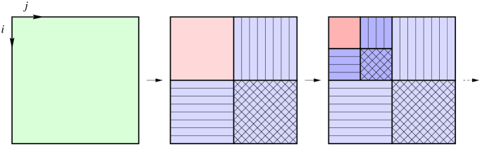
Figure 6: Action of the 2-D fast wavelet transform and structure of the transformed data. The original data and the approximations are represented without patterns. The details corresponding to vertical/horizontal/diagonal variations are represented by patterns of horizontal/vertical/diagonal lines (features along a certain direction have maximum gradient along the perpendicular direction).

4.3 Fast wavelet transform

From the computational point of view, the choice of the wavelet corresponds to the choice of a set of filters for the fast wavelet transform and its inverse. For a bi-orthogonal wavelet, they are: the high-pass and low-pass decomposition filters $\tilde{g}_{i}$ and $\tilde{h}_{i}$, and the high-pass and low-pass reconstruction filters $g_{i}$ and $h_{i}$, respectively. In the orthogonal case, $\tilde{g}_{i}=g_{i}$ and $\tilde{h}_{i}=h_{i}$. The coefficients of $\tilde{h}_{i}$ and $h_{i}$ are tabulated and centred as close as possible to $i=0$, while those of $\tilde{g}_{i}$ and $g_{i}$ are computed from the relations $\tilde{g}_{i+1}=(-1)^{i+1}h_{-i}$ and $g_{i+1}=(-1)^{i+1}\tilde{h}_{-i}$. The filters are padded with zeros so as to be defined for $i=-M,\ldots,M$ ($M$ even), and to be consistent with the formulae for the transforms. In particular, ‘bior 4.4’ and ‘rbio 4.4’ have $M=6$, while ‘bior 6.8’ and ‘rbio 6.8’ have $M=10$. (The detailed relations of such filters to the wavelets and scaling functions are very complicated and irrelevant to our context; see Goedecker 1998.)

One step of the (forward) fast wavelet transform replaces the current approximation $A_{i}(N_{\mathrm{t}})$, of size $N_{\mathrm{t}}$, with a coarser approximation $A_{i}(N_{\mathrm{t}}/2)$ and detail $D_{i}(N_{\mathrm{t}}/2)$, of size $N_{\mathrm{t}}/2$:

$$A_{i}(N_{\mathrm{t}}/2)=\sum_{j=-M+1}^{M}\tilde{h}_{j}A_{j+2i}(N_{\mathrm{t}})\,,$$ (7)

$$D_{i}(N_{\mathrm{t}}/2)=\sum_{j=-M+1}^{M}\tilde{g}_{j}A_{j+2i}(N_{\mathrm{t}})\,,$$ (8)

where the index $j+2i$ is wrapped around when it gets out of the range (periodic boundary conditions; see Goedecker 1998). Initially, $N_{\mathrm{t}}=N_{\mathrm{d}}$ and $A_{i}=X_{i}$, $X_{i}(N_{\mathrm{d}})$ being the original data. The transform ends when $N_{\mathrm{t}}=N_{\mathrm{t\,min}}$, so that the transformed data $Y_{i}(N_{\mathrm{d}})$ consist of the coarse approximation $A_{i}(N_{\mathrm{t\,min}}/2)$ and the sequence of finer and finer details $D_{i}(N_{\mathrm{t\,min}}/2)$, $D_{i}(N_{\mathrm{t\,min}})$, …, $D_{i}(N_{\mathrm{d}}/2)$. Note that $N_{\mathrm{t\,min}}$ is a free parameter of the code. If we assume that $N_{\mathrm{d}}$ is a power of 2, then $N_{\mathrm{t\,min}}$ is also a power of 2 and such that $2\leq N_{\mathrm{t\,min}}\leq N_{\mathrm{d}}$. A complete transform corresponds to $N_{\mathrm{t\,min}}=2$, but this value does not necessarily mean a good de-noising. A more general assumption is that $N_{\mathrm{d}}$ contains a power of two, which has obvious implications for $N_{\mathrm{t\,min}}$. Data of different size can be padded (see Sect. 6).

How does the value of the parameter $N_{\mathrm{t\,min}}$ affect de-noising? The reference case illustrated in Fig. 3 corresponds to $N_{\mathrm{t\,min}}=64$ ($N_{\mathrm{d}}=2048$). Fig. 5 shows the effects of other values. For $N_{\mathrm{t\,min}}=2048$, only the smallest-scale noise is removed so the processed data are nearly as noisy as the original data. For $N_{\mathrm{t\,min}}=128$, there is residual noise on large scales, and the resulting signal-to-noise ratio and de-noising factor are worse than in the reference case. For $N_{\mathrm{t\,min}}=2$, the de-noising is complete and nearly as good as for $N_{\mathrm{t\,min}}=64$. Nevertheless, there are large anomalous coefficients in the five coarsest details, which exceed the threshold, and small anomalies in the de-noised data.

Let us then explain which values of $N_{\mathrm{t\,min}}$ imply a good de-noising. It must be $N_{\mathrm{t\,min}}\ll N_{\mathrm{d}}$, otherwise de-noising is incomplete; and besides $N_{\mathrm{t\,min}}\ga 4M$, otherwise the wavelet becomes too dilated in comparison with the size of the data and wrap-around effects become significant. (Cosmological simulations are peculiar in this context; see Sect. 5.3.) The best value of $N_{\mathrm{t\,min}}$ depends on the problem and can be found through the optimization trial discussed in Sect. 6.

Finally, we point out the (non-obvious) differences between the 2-D or 3-D fast wavelet transform and the 1-D case. Fig. 6 shows how the transform acts on 2-D data. In general, given $n$-D data of size $N_{\mathrm{d}}^{n}$, the first step of the transform decomposes them into $2^{n}$ parts of size $(N_{\mathrm{d}}/2)^{n}$: 1 approximation and $2^{n}-1$ details, one for each axis and each diagonal. It is done by 1-D transforming the data along each index, for all values of the other indices, consecutively. Then the discussion basically follows the 1-D case, except that the complexity of the transform increases by a factor of $n\,2^{n-1}/(2^{n}-1)$ with respect to $4MN_{\mathrm{d}}^{n}$. The generalization to data of size $N_{\mathrm{d}1}\cdots N_{\mathrm{d}n}$ is plain.

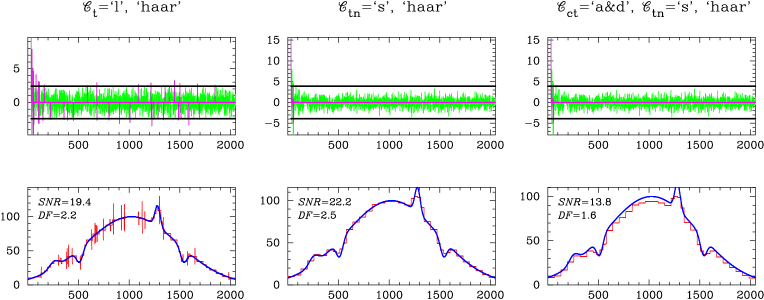
Figure 7: Original and thresholded wavelet coefficients (top), and de-noised data vs. the model data (bottom) for various thresholding options and the ‘haar’ wavelet. Also specified are the signal-to-noise ratio $\mathit{SNR}$ in the de-noised data and the de-noising factor $\mathit{DF}$. The reference case illustrated in Fig. 3 corresponds to $\mathcal{C}_{\mathrm{t}}=\mbox{`h'}$, $\mathcal{C}_{\mathrm{ct}}=\mbox{`d'}$, $\mathcal{C}_{\mathrm{tn}}=\mbox{`h'}$ and the ‘bior 4.4’ wavelet [for the corresponding ‘haar’ case cf. Fig. 4 (left)].

4.4 Thresholding of the wavelet coefficients

The heart of de-noising consists of identifying a correct threshold, and deciding which type of wavelet coefficients are to be thresholded and how. Note the difference between thresholding and smoothing, where the detail coefficients below a given scale are set to zero independent of their value. In the following, we discuss thresholding and introduce the options of the code.

As pointed out in Sect. 4.2, a correct threshold can be identified if the wavelet is orthogonal, or quasi-orthogonal. The threshold $T$ is proportional to the standard deviation of noise $\sigma$, and the proportionality factor $K$ depends on the size of the data:

$$T=K(N_{\mathrm{d}})\,\sigma\,.$$ (9)

If the standard deviation is not given ($\mathcal{C}_{\mathrm{sd}}=\mbox{`ng'}$), as in the case of Gaussian white noise, then it is robustly estimated through the median absolute deviation of the finest detail:

$$\sigma\simeq\frac{1}{0.6745}\,\mathit{MAD}[D_{i}(N_{\mathrm{d}}/2)]\,.$$ (10)

A robust estimator and the finest detail are used for minimizing the contribution of outlying wavelet coefficients, which are not caused by noise. If the standard deviation is given ($\mathcal{C}_{\mathrm{sd}}=\mbox{`g'}$), as in the case of Poissonian noise, then

$$\sigma\simeq 1\,.$$ (11)

Concerning $K(N_{\mathrm{d}})$, it is rigorously determined so that the threshold matches both the noise level and the significance level of the wavelet coefficients, according to probability criteria. We can decide between two functional forms for $K(N_{\mathrm{d}})$. One corresponds to a higher threshold ($\mathcal{C}_{\mathrm{t}}=\mbox{`h'}$), which is more effective but less safe:

$$K(N_{\mathrm{d}})=\sqrt{2\ln N_{\mathrm{d}}}\,.$$ (12)

The other corresponds to a lower threshold ($\mathcal{C}_{\mathrm{t}}=\mbox{`l'}$), and is approximated analytically as:

$$K(N_{\mathrm{d}})\simeq\left\{\begin{array}[]{ll}0&\mbox{if\ }N_{\mathrm{d}}\leq 32\,,\\ 0.3936+0.1829\log_{2}N_{\mathrm{d}}&\mbox{else}\,.\end{array}\right.$$ (13)

Next, the wavelet coefficients to threshold can be either the details ($\mathcal{C}_{\mathrm{ct}}=\mbox{`d'}$):

$$W_{i}=D_{i}(N_{\mathrm{t\,min}}/2),\ldots,D_{i}(N_{\mathrm{d}}/2)\,;$$ (14)

or the approximation & the details ($\mathcal{C}_{\mathrm{ct}}=\mbox{`a\&d'}$):

$$W_{i}=A_{i}(N_{\mathrm{t\,min}}/2),D_{i}(N_{\mathrm{t\,min}}/2),\ldots,D_{i}(N_{\mathrm{d}}/2)\,.$$ (15)

The last option concerns the thresholding (method), named as in the literature. It can be either hard ($\mathcal{C}_{\mathrm{tn}}=\mbox{`h'}$):

$$\overline{W}_{i}=\left\{\begin{array}[]{ll}0&\mbox{if\ }|W_{i}|\leq T\,,\\ W_{i}&\mbox{else}\,;\end{array}\right.$$ (16)

or soft ($\mathcal{C}_{\mathrm{tn}}=\mbox{`s'}$):

$$\overline{W}_{i}=\left\{\begin{array}[]{ll}0&\mbox{if\ }|W_{i}|\leq T\,,\\ \mathrm{sign}(W_{i})(|W_{i}|-T)&\mbox{else}\,.\end{array}\right.$$ (17)

So $\mathcal{C}_{\mathrm{tn}}=\mbox{`s'}$ means that even the wavelet coefficients above $T$ are thresholded, and this is done shrinking them by $T$.

How do the thresholding options affect de-noising? The reference case illustrated in Fig. 3 corresponds to $\mathcal{C}_{\mathrm{t}}=\mbox{`h'}$, $\mathcal{C}_{\mathrm{ct}}=\mbox{`d'}$ and $\mathcal{C}_{\mathrm{tn}}=\mbox{`h'}$ ($\mathcal{C}_{\mathrm{sd}}=\mbox{`ng'}$). Fig. 7 shows the effects of other options. As the situation is degenerate, we consider the ‘haar’ wavelet instead of ‘bior 4.4’, since it reduces the degeneracy and its effects have already been shown [cf. Fig. 4 (left)]. For $\mathcal{C}_{\mathrm{t}}=\mbox{`l'}$, the threshold is exceeded by several noisy detail coefficients, which give rise to spikes in the de-noised data. For $\mathcal{C}_{\mathrm{tn}}=\mbox{`s'}$, the soft thresholding of the detail coefficients over-regularizes the de-noised data, softening the maxima and minima. If in addition $\mathcal{C}_{\mathrm{ct}}=\mbox{`a\&d'}$, then the thresholding of the approximation coefficients biases the de-noised data.

Let us then explain which thresholding options imply a good de-noising. We suggest the more effective option $\mathcal{C}_{\mathrm{t}}=\mbox{`h'}$ for standard data, unless they are expected to have meaningful irregularities below the maximum noise level; while we recommend the safer option $\mathcal{C}_{\mathrm{t}}=\mbox{`l'}$ for simulations. In addition, it must be $\mathcal{C}_{\mathrm{ct}}=\mbox{`d'}$ and $\mathcal{C}_{\mathrm{tn}}=\mbox{`h'}$, otherwise the de-noised data get biased and over-regularized, respectively. (In advanced de-noising, $\mathcal{C}_{\mathrm{ct}}$ and $\mathcal{C}_{\mathrm{tn}}$ are replaced by a more useful parameter; see Sect. 5.1.) Finally, it is natural to opt for $\mathcal{C}_{\mathrm{sd}}=\mbox{`ng'}$ in the case of Gaussian white noise, and for $\mathcal{C}_{\mathrm{sd}}=\mbox{`g'}$ in the case of Poissonian noise. If the Poissonian data have a sufficiently high signal-to-noise ratio, such that the estimated $\sigma\simeq 1$, then $\mathcal{C}_{\mathrm{sd}}=\mbox{`ng'}$ fine-tunes the accuracy of de-noising. The algorithm gets slightly slower since the computation of the median has complexity $O(N_{\mathrm{d}})$. Therefore $\mathcal{C}_{\mathrm{sd}}=\mbox{`ng'}$ may be a better option than $\mathcal{C}_{\mathrm{sd}}=\mbox{`g'}$ for standard data, not for simulations (where the signal-to-noise ratio is low and speed is a primary factor).

Finally, thresholding in 2D or 3D is similar to the 1-D case and the generalization to data of size $N_{\mathrm{d}1}\cdots N_{\mathrm{d}n}$ is plain, except for the more complicated structure of the wavelet coefficients.

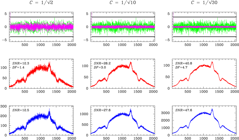
Figure 8: Partial de-noising at a pre-assigned level. Original and thresholded wavelet coefficients (top), and de-noised data (middle) for various values of the contraction parameter $C$; also shown for comparison are realizations of Poissonian data with $1/C^{2}$ times more ‘counts’ than in the original noisy data (bottom). The signal-to-noise ratio $\mathit{SNR}$ and the de-noising factor $\mathit{DF}$ are specified. The reference case illustrated in Fig. 3 corresponds to $C=0$ (total de-noising). The implication for simulations is explained in the text.

4.5 Inverse fast wavelet transform

One step of the inverse (backward) fast wavelet transform replaces the current approximation $A_{i}(N_{\mathrm{t}}/2)$ and coarsest detail $D_{i}(N_{\mathrm{t}}/2)$ with a finer approximation $A_{i}(N_{\mathrm{t}})$:

$$A_{2i}(N_{\mathrm{t}})=\!\!\!\!\!\sum_{j=-M/2}^{M/2-1}\!\!\!\!\!h_{2j}A_{i-j}(N_{\mathrm{t}}/2)+g_{2j}D_{i-j}(N_{\mathrm{t}}/2)\,,$$ (18)

$$A_{2i+1}(N_{\mathrm{t}})=\!\!\!\!\!\sum_{j=-M/2}^{M/2-1}\!\!\!\!\!h_{2j+1}A_{i-j}(N_{\mathrm{t}}/2)+g_{2j+1}D_{i-j}(N_{\mathrm{t}}/2)\,,$$ (19)

where the index $i-j$ is wrapped around when it gets out of the range (see Goedecker 1998), $N_{\mathrm{t}}$ goes from $N_{\mathrm{t\,min}}$ to $N_{\mathrm{d}}$, and so on (see Sect. 4.3).

The inverse fast wavelet transform can be used for plotting wavelets, as in Fig. 1. Consider the data $X_{i}=\delta_{in}$ and the inverse transformed data $Y_{i}$. A discrete approximation of $\psi_{\mathrm{rec}}(x)$ or $\phi_{\mathrm{rec}}(x)$ can be computed from $Y_{i}$ through the following operations: scaling, translation, normalization and possibly wrap-around. The accuracy of the approximation, the type of function and the parameters of the operations depend on $N_{\mathrm{d}}$, $N_{\mathrm{t\,min}}$ and $n$. Including the reverse set of filters produces $\psi_{\mathrm{dec}}(x)$ or $\phi_{\mathrm{dec}}(x)$. In Fig. 1, we have set: $N_{\mathrm{d}}=2^{14}$, $N_{\mathrm{t\,min}}=2^{7}$, $n=3N_{\mathrm{t\,min}}/4$ for the wavelet plots and $n=N_{\mathrm{t\,min}}/4$ for the scaling-function plots. In both plots, the discrete argument is $x_{i}=(i-b)/a$ and the function is $f(x_{i})=\sqrt{a}\,Y_{i}$, with $a=2N_{\mathrm{d}}/N_{\mathrm{t\,min}}$ and $b=N_{\mathrm{d}}/2$. Such a set-up provides an accurate approximation and avoids wrap-around, and thus it can be used for plotting wavelets in general.

4.6 Post-processing of the data

The data should be post-processed in the case of Poissonian noise. Post-processing consists of inverse Anscombe transforming plus two corrections. The first correction is needed if the Anscombe transformation fails locally (see Sect. 4.1), giving rise to small negative values in the de-noised data. We can correct such values by setting them to zero. The second correction is required because the Anscombe transformation introduces a local bias in the data. That is, if $\mu_{\mathrm{P}}$ is the local mean of $Y_{\mathrm{P}}$ and $\mu_{\mathrm{G}}$ is the local mean of $Y_{\mathrm{G}}$, the mean $\mu_{\mathrm{P}}^{\prime}$ estimated by inverse transforming $\mu_{\mathrm{G}}$ is not equal to $\mu_{\mathrm{P}}$, and their difference is the local bias of the transformation. Starck et al. (1998) have implied that the bias is multiplicative and unbounded, while Kolaczyk (1997) has implied that the bias is additive and bounded but has not estimated it. Indeed, the comprehensive book by Stuart & Ord (1991) shows that the bias of the Anscombe transformation is additive and bounded, and can be estimated analytically:

$$\mathit{BIAS}\simeq-\frac{1}{4}\left(1-\frac{1}{N_{\mathrm{d}}}\right)\sigma_{\mathrm{G}}^{2}\,.$$ (20)

This means that, with very little effort, we can subtract the bias almost completely from the de-noised data. And, if even a slight global bias is unacceptable, then we can compute it numerically and subtract it completely from the de-noised data.

5 EXPLORING ADVANCED DE-NOISING

Consider a simulation where the particle distribution is denoised at each timestep. If initially the de-noising factor is $\mathit{DF}_{0}$, then the de-noised model has the same signal-to-noise ratio as a noisy model with $\mathit{DF}_{0}^{2}$ times more particles. This follows from the fact that the noise is basically Poissonian, and hence the signal-to-noise ratio is proportional to the square root of the average number of particles per cell. Besides, as $\mathit{DF}$ depends more on the de-noising ability of the wavelet method than on the characteristics of the particle distribution, we can draw a more general conclusion: the de-noised simulation itself is roughly equivalent to a noisy simulation with $\mathit{DF}_{0}^{2}$ times more particles (cf. Paper I). Until now we have learned how to de-noise so as to get the largest $\mathit{DF}$ (see Sects 3.2 and 4). On the other hand, in simulations we do not always want to suppress noise totally. We may instead want to reduce it partially in order to understand and control its effects. In this section, we learn how to carry out such an advanced de-noising.

5.1 Partial de-noising at a pre-assigned level

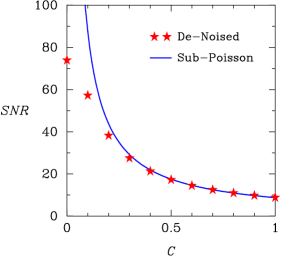
Figure 9: Accuracy of partial de-noising at a pre-assigned level. The signal-to-noise ratio $\mathit{SNR}$ is shown as a function of the contraction parameter $C$ for the de-noised data and for sub-Poissonian data. The sub-Poissonian data have local standard deviation $\sigma_{\mathrm{sub}}=C\sqrt{\mu_{\mathrm{sub}}}$ and local mean $\mu_{\mathrm{sub}}=\mu_{\mathrm{P}}$, where $\mu_{\mathrm{P}}$ refers to the original data with Poissonian noise; hence $(\mathit{SNR})_{\mathrm{sub}}=(\mathit{SNR})_{\mathrm{P}}/C$. The accuracy is better than 10% for $C\ga 1/\sqrt{20}$, and it gets worse than 20% for $C\la 1/\sqrt{40}$. The implication for simulations is explained in the text.

5.1.1 Method and implementation

Can we de-noise a simulation so as to make it equivalent to a simulation with $\Gamma$ times more particles, for a pre-assigned level $\Gamma$? Yes! And the idea is the following. Recall what hard thresholding of the details means (see Sect. 4.4), and consider the wavelet coefficients below the threshold. If we contract them by $C$, instead of setting them to zero, then the noise level decreases by the same factor whereas the ‘signal’ does not change. Hence the signal-to-noise ratio increases by a factor of $1/C$, and the simulation becomes equivalent to a simulation with $1/C^{2}$ times more particles. Thus the problem is solved if we set $C=1/\sqrt{\Gamma}$. (For an analogous thresholding in the context of speech signals see Storm 1998.)

We now illustrate this idea in the simple, but instructive, context of standard data. Fig. 8 shows that partial de-noising at a pre-assigned level works as expected. Note that this type of de-noising is meant to turn data with Poissonian noise into ‘sub-Poissonian’ data. In such data the original Poissonian deviations from the local mean are contracted by $C$, while obviously the de-noised data are subject to an estimation error. Fig. 9 shows that, as expected, the accuracy of partial de-noising at a pre-assigned level is very good except for $C\la 2/(\mathit{DF})_{\mathrm{tot}}$, where $(\mathit{DF})_{\mathrm{tot}}$ refers to the case of total de-noising ($C=0$).

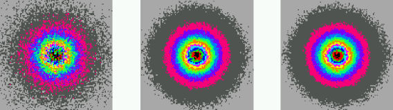
Figure 10: Partial de-noising at a pre-assigned level in action: comparison between the initial models. The set of simulation models has a physical grid of $N_{\mathrm{c}}=N_{\mathrm{d}}^{2}=256^{2}$ cells and cell size $\Delta_{\mathrm{c}}=0.25$ kpc. The particle distribution is shown for the noisy model with $N=10^{5}$ particles (left), the noisy model with $N=10^{6}$ (middle), and the de-noised model with $N=10^{5}$ and contraction parameter $C=1/\sqrt{10}$ (right). In each model the signal-to-noise ratio is $\mathit{SNR}\simeq 5.7,17.8,17.1$, respectively. As expected, the accuracy of partial de-noising at a pre-assigned level is very good for such initial models.

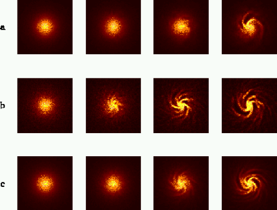
Figure 11: Partial de-noising at a pre-assigned level in action: fragmentation of a cool galactic disc. a: de-noised simulation with $N=10^{5}$ and $C=1/\sqrt{10}$; b: noisy simulation with $N=10^{5}$; c: noisy simulation with $N=10^{6}$. The initial models are the same as in Fig. 10. For each simulation, the particle distribution is shown from 0 Myr to 150 Myr at intervals of 50 Myr (from left to right). The time $\tau$ at which the initial axial symmetry breaks is a measure of the effect of noise on the simulation: a long $\tau$ means a weak effect. As expected, $\tau$ increases from b to c; we also notice that $\tau$ is a little longer in a than in c.

5.1.2 Bench-marks

Let us then explore this idea in simulations of disc galaxies. The examination is based on four bench-marks, originally introduced in Paper I.

1. The first natural bench-mark is the comparison between the initial models.

2. The second bench-mark concerns the fragmentation of a cool galactic disc, which is the onset of a gravitational instability (see, e.g., Binney & Tremaine 1987). A rotating disc with low velocity dispersion is gravitationally unstable and therefore sensitive to perturbations, which are amplified and break the initial axial symmetry of the system (e.g., Semelin & Combes 2000; Huber & Pfenniger 2001). The time that characterizes symmetry breaking clearly depends on the initial amplitude of the perturbations, for small perturbations need a long time to grow into an observable level. In particular, this is true for the fluctuations imposed by granular initial conditions. Thus the symmetry-breaking time is a clear diagnostic for quantifying the effect of noise on the simulation.

3. The third bench-mark concerns the heating following the fragmentation. This is a fundamental process in the dynamical evolution of disc galaxies, which is induced by gravitational instabilities via the outward transport of angular momentum and energy (see, e.g., Binney & Tremaine 1987). Therefore this bench-mark has a clear physical motivation. When spiral gravitational instabilities reach a sufficiently large amplitude, the velocity dispersion of the disc starts to increase by collective relaxation (e.g., Zhang 1998; Griv, Gedalin & Yuan 2002). The heat produced in a dynamical time is low if the initial amplitude of the instabilities is small. Thus the increase of velocity dispersion is another diagnostic for quantifying the effect of noise on the simulation.

4. The fourth bench-mark concerns the accretion following the fragmentation. This is also a fundamental process in the dynamical evolution of disc galaxies (see, e.g., Binney & Tremaine 1987). Therefore this bench-mark also has a clear physical motivation. The amplification of spiral gravitational instabilities produces not only heating but also re-distribution of matter in the disc, which appears more evidently as accretion near the centre (e.g., Zhang 1998; Griv et al. 2002). The mass accreted in a dynamical time is low if the initial amplitude of the instabilities is small. Thus the peak of mass density is still another diagnostic for quantifying the effect of noise on the simulation.

We consider the same basic simulation as in Paper I, which has $N=10^{5}$ particles. We de-noise it choosing the ‘rbio 6.8’ wavelet, and setting $N_{\mathrm{t\,min}}=16$ and $C=1/\sqrt{10}$, so as to make it equivalent to a simulation with 10 times more particles (the thresholding options are the usual ones for simulations; see Sect. 4.4). The conservation of angular momentum and energy is not significantly affected. In fact, the deviations are less than 0.02% and 0.04% per dynamical time, respectively, and compare well with those typical of the code (Combes et al. 1990). We also run the noisy simulation with $N=10^{6}$. This suite of simulations is sufficient for the present purpose. For further comparison see the extensive survey presented in Paper I (the de-noised simulation has $C=0$).

Figs 10–13 illustrate that partial de-noising at a pre-assigned level works as expected, and the agreement is very good, except that the de-noised simulation takes a little longer time to form the initial transient structures (cf. Fig. 11). The reason for this imperfection is twofold: it concerns the de-noising itself (threshold) and the initial conditions (noisy starts).

Threshold. At the beginning of the simulation, there is no way to differentiate instabilities from amplified noisy fluctuations. Thresholding weakens the initial instabilities until the relevant wavelet coefficients exceed the threshold. The usual threshold tends to be slightly too high, and therefore the onset of the initial instabilities is delayed.

Noisy starts. We know that the initial particle positions and velocities are noisy. We also know that the particle density is partially de-noised, and the computed field has a consistent noise level. This means that the excess of noise remains confined in phase space and does not propagate dynamically. In fact, in the de-noised simulation the amplitude of the statistical fluctuations is similar to the noisier case, whereas the evolution of the relevant quantities is similar to the less noisy case (cf. Figs 12 and 13). On the other hand, the excess of noise makes instabilities less coherent, and therefore it delays their onset.

Thus it is hard to evaluate the accuracy of partial de-noising at a pre-assigned level for simulations, even if the accuracy is better than a few per cent for the initial models (cf. Fig. 10). But the conclusion is strong anyway: our method, and code, can be used for understanding and controlling the effects of noise on simulations.

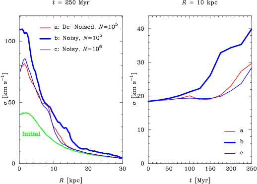
Figure 12: Partial de-noising at a pre-assigned level in action: heating following the fragmentation of a cool galactic disc. The simulations are the same as in Fig. 11. The velocity dispersion $\sigma$ is shown as a function of radius $R$ at the initial and final times, and as a function of time $t$ at an intermediate radius. The increase of velocity dispersion $\Delta\sigma(R)$ from the initial to the final value is a measure of the effect of noise on the simulation: a small $\Delta\sigma$ means a weak effect. In the simulations, except b, heating is significant only for $R\la 12$ kpc. As expected, $\Delta\sigma_{\mathrm{b}}>\Delta\sigma_{\mathrm{c}}$ and $\Delta\sigma_{\mathrm{a}}\approx\Delta\sigma_{\mathrm{c}}$.

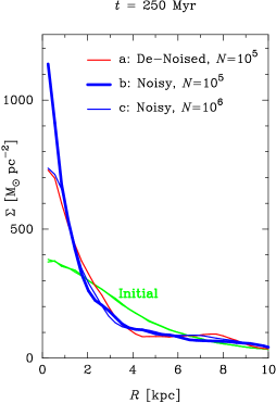
Figure 13: Partial de-noising at a pre-assigned level in action: accretion following the fragmentation of a cool galactic disc. The simulations are the same as in Fig. 11. The mass density $\Sigma$ is shown as a function of radius $R$ at the initial and final times. The peak of final mass density $\hat{\Sigma}$ near the centre is a measure of the effect of noise on the simulation: a low $\hat{\Sigma}$ means a weak effect. As expected, $\hat{\Sigma}_{\mathrm{b}}>\hat{\Sigma}_{\mathrm{c}}$ and $\hat{\Sigma}_{\mathrm{a}}\approx\hat{\Sigma}_{\mathrm{c}}$.

5.1.3 Controlling the effectiveness of de-noising

Before exploring more advanced aspects of de-noising, let us reflect on the main differences between partial de-noising at a pre-assigned level and total de-noising, and explain what we mean by noise control (or analogous terms). Consider a simulation with, say, $N=10^{5}$ particles. And suppose that we decide beforehand to make it equivalent to a simulation with, say, $N_{\mathrm{pre}}=1.8\times 10^{6}$ particles (pre-assigned number). Then we set the contraction parameter $C=1/\sqrt{18}$, and run the simulation. The partially de-noised model will accurately mimic a noisy model with $\Gamma=18$ times more particles. This is noise control. On the other hand, the accuracy of partial de-noising at a pre-assigned level deteriorates for small $C$ (cf. Fig. 9 and its discussion). In the limit $C\rightarrow 0$ the effectiveness of de-noising becomes maximum, but we cannot predict it with sufficient accuracy unless we compare the initial models quantitatively (see Paper I). If the method were perfect we would have an improvement in the equivalent number of particles by a factor of $1/C^{2}\rightarrow\infty$, whereas in practice the improvement is by a factor of about 100 (cf. Paper I). In such a case we do not have control over noise, but we exploit total (maximum) de-noising.

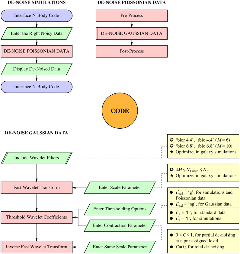
Figure 14: Flowchart of the code.

5.2 Partially noisy starts and adaptive de-noising

Can we achieve an even better noise control? Yes, in principle, and the idea is the following. We should first impose appropriate initial conditions so as to make the model equivalent to a model with $\Gamma$ times more particles, without de-noising it. Such partially noisy starts can be generated by setting up a fraction $1/\Gamma$ of the particles with noisy starts, and the rest with quiet starts (quiet starts are common in plasma simulations; see, e.g., Dawson 1983; Birdsall & Langdon 1991). Doing so, the initial particle distribution is basically sub-Poissonian and its signal-to-noise ratio is higher than in the Poissonian case by a factor of $\sqrt{\Gamma}$. On the other hand, the noise has a natural tendency to become fully Poissonian in few dynamical times, as a reaction of the system to the imposed order and hence reduced entropy. We should then de-noise the simulation consistently. At the initial time, the threshold $T$ is lower than the usual one by a factor of $1/\sqrt{\Gamma}$ and the contraction parameter $C$ is unity (no de-noising). When the noise level increases, $T$ should be increased accordingly and $C$ should be decreased in inverse proportion (in the case of quiet starts, $C=0$; see also Paper I). Such an adaptive de-noising is not yet implemented in the code.

5.3 Partial de-noising up to a given scale

Cosmological simulations are peculiar with respect to galaxy and plasma simulations. The initial conditions consist of setting up a quiet uniform particle distribution, and of imposing small random fluctuations with Gaussian statistics and a given power spectrum (e.g., Efstathiou et al. 1985; Sylos Labini et al. 2003). Such fluctuations are amplified by gravitational instability and form stuctures. On the other hand, Poissonian noise develops on the same time-scale and therefore affects structure formation. The onset of Poissonian noise is especially quick in cold dark matter simulations, where structures form bottom-up and the first virialized systems contain a small number of particles (e.g., Binney & Knebe 2002; Diemand et al. 2004).

Thus de-noising cosmological simulations is a very complex and demanding problem: the method should remove noise without affecting the physical random fluctuations. An ad hoc solution for cold dark matter simulations may be to de-noise them only over a range of scales that is adapted to the phase of clustering: from the cell size to the size of the structures that have formed latest (see Paper I). Partial de-noising up to a given scale is implemented in the code, but it is not tested in this context; the scale parameter is $N_{\mathrm{t\,min}}$ (see Sect. 4.3). An upper scale of $2^{n}$ cell sizes corresponds to $N_{\mathrm{t\,min}}=N_{\mathrm{d}}/2^{n}$. At the beginning of the simulation, before the first virialized systems have formed, the upper scale should match the smallest physical scale unaffected by the $N$-body method, so $N_{\mathrm{t\,min}}$ should be set to $N_{\mathrm{d}}/2$ or $N_{\mathrm{d}}/4$. Analogous solutions may be found in the context of other cosmological models.

6 HOW TO USE THE CODE

A flowchart of the code is illustrated in Fig. 14 (the symbols are standard; see, e.g., Nyhoff & Leestma 1997). It summarizes the most useful information given in Sects 4 and 5, without repeating the relevant definitions. In this section, we discuss such practical points in detail. Supplementary information is given in the readme-file of the code distribution.

The code can be used for de-noising $N$-body simulations, and 1D–3D standard data with Poissonian noise or additive white Gaussian noise. It contains include-files for many orthogonal and bi-orthogonal wavelet filters, and also routines for the fast wavelet transform and its inverse. The number of data points should contain powers of two. Data of different size can be padded: add zeros, or extend the data so that their boundary values match smoothly. Smooth padding is better because it reduces wrap-around effects. Data with multiplicative and/or coloured Gaussian noise can also be de-noised. In the first case, pre-process the data by taking their logarithm, de-noise them in the usual way and post-process. In the second case, compute the standard deviation of noise on each scale from the corresponding detail, and threshold the wavelet coefficients accordingly.

We now explain how to include our add-on code in particle-mesh $N$-body codes (e.g., Combes et al. 1990; Pfenniger & Friedli 1993; Klypin & Holtzman 1997). The proper de-noising subroutine should be called just after the mass/charge assignment. Note that the right argument is the number of particles per cell in the active grid, not the mass/charge distribution in the whole mesh. Therefore the subroutine needs a simple interface for the conversion of such arrays. The specific form of interface depends on Fortran details. If there are various particle species, which represent components with different collision properties, then each species can have its own type of de-noising. The case of polar grids is similar to the Cartesian case. In fact, for our purpose we can regard the space spanned by the cell indices as Cartesian and the particle distribution defined there as evenly sampled. In addition, the boundary values of the particle distribution match smoothly, except near the intersections between the radial boundaries and the equatorial plane. So smooth padding may be justified even if the number of radial cells already contains a power of two. In order to reduce wrap-around effects significantly, the thickness of the padding layer should be comparable to the size of the wavelet filters. Note that such extra cells are only used for de-noising purposes and do not enter into the $N$-body computation itself. The case of other grid geometries is analogous. It is not yet clear how to include our add-on code in other types of $N$-body codes.

Let us finally remark that the physical performance of the code depends on how it is used. In order to get a very good performance, follow the guide-lines of Sects 4 and 5 and the practical advice of this section. The performance can be optimized in the case of galaxy simulations, since the initial model is noisy and the theoretical particle distribution is known. The degrees of freedom are the choice of the wavelet and the value of the scale parameter (cf. Sects 4.2 and 4.3). The optimization consists of a simple trial: vary such degrees of freedom so as to get the largest de-noising factor, and check the visual quality of the de-noised model. In the case of cosmological simulations of structure formation in the early Universe, the value of the scale parameter is a critical issue (cf. Sect. 5.3), while an appropriate choice of the wavelet may be guessed considering the characteristics of such structures. For example, in cold dark matter simulations we would choose the ‘bior 4.4’ wavelet (cf. Fig. 1) since the haloes that form are cuspy. In the cases of plasma simulations and standard data, we cannot give more specific instructions than those of Sects 4 and 5.

7 CONCLUSIONS

$N$-body simulations of structure formation in the early Universe, of galaxies and plasmas are limited crucially by noise, whose effects are subtle and not yet fully understood. In Paper I, we have introduced an innovative multi-scale method of noise reduction based on wavelets, which promises marked advances in those contexts. In this paper, we have discussed such a method and its code implementation. We have also explained how to include our code in the simulator’s $N$-body code, and how to use it for de-noising standard data. The code is available on request from the first author. The major conclusions of this paper are pointed out below.

1. This is the first wavelet add-on code designed for de-noising $N$-body simulations, and as such is meant to be a building block for more elaborate de-noising codes. We hope to have stimulated curiosity about the uses of our code, and we challenge simulators to apply it to physical problems where noise must be suppressed or controlled.

2. The strength of the code is twofold. It improves the performance of simulations up to two orders of magnitude (cf. Paper I). Besides, it allows controlling the effects of noise: the $N$-body simulation can be made equivalent to a simulation with a pre-assigned number of particles $N_{\mathrm{pre}}$, for $N_{\mathrm{pre}}/N$ larger than unity and spanning one order of magnitude.

3. The weakness or rather small imperfection of the code is that noise-generated instabilities are not reproduced very well, in contrast to the induced dynamical evolution. Obviously, errors may follow from an incorrect use of the code.

4. Finally, we believe that the performance of simulations can be further improved with a more appropriate pre-processing of the data. Fryźlewicz & Nason (2004) have shown that the Haar-Fisz transformation is better than the Anscombe transformation for pre-processing data with Poissonian noise, and that the computational time is comparable (see also Fryzlewicz 2003). Work is in progress to investigate other relevant properties and uses of this transformation, before including it in our code.

References

- [1] Addison P. S., 2002, The Illustrated Wavelet Transform Handbook: Introductory Theory and Applications in Science, Engineering, Medicine and Finance. Institute of Physics Publishing, Bristol
- [2] Anscombe F. J., 1948, Biometrika, 35, 246
- [3] Arter W., 1995, Rep. Prog. Phys., 58, 1
- [4] Bergh J., Ekstedt F., Lindberg M., 1999, Wavelets. Studentlitteratur, Lund
- [5] Bevington P. R., Robinson D. K., 1992, Data Reduction and Error Analysis for the Physical Sciences. McGraw-Hill, New York
- [6] Binney J., 2004, MNRAS, 350, 939
- [7] Binney J., Knebe A., 2002, MNRAS, 333, 378
- [8] Binney J., Tremaine S., 1987, Galactic Dynamics. Princeton University Press, Princeton (errata in astro-ph/9304010)
- [9] Birdsall C. K., Langdon A. B., 1991, Plasma Physics via Computer Simulation. Institute of Physics Publishing, Bristol
- [10] Byrd G., 1995, in Hunter J. H. Jr., Wilson R. E., eds, Ann. N. Y. Acad. Sci. 773, Waves in Astrophysics. N. Y. Acad. Sci., N. Y., p. 302
- [11] Combes F., Debbasch F., Friedli D., Pfenniger D., 1990, A&A, 233, 82
- [12] Daubechies I., 1992, Ten Lectures on Wavelets. SIAM, Philadelphia
- [13] Dawson J. M., 1983, Rev. Mod. Phys., 55, 403
- [14] Dehnen W., 2001, MNRAS, 324, 273
- [15] Diemand J., Moore B., Stadel J., Kazantzidis S., 2004, MNRAS, 348, 977
- [16] Efstathiou G., Davis M., Frenk C. S., White S. D. M., 1985, ApJS, 57, 241
- [17] Fryzlewicz P. Z., 2003, PhD thesis, University of Bristol
- [18] Fryźlewicz P., Nason G. P., 2004, J. Comput. Graph. Stat., in press
- [19] Goedecker S., 1998, Wavelets and Their Application for the Solution of Partial Differential Equations in Physics. Presses Polytechniques et Universitaires Romandes, Lausanne
- [20] Gonzalez R. C., Woods R. E., 2002, Digital Image Processing. Prentice Hall, Upper Saddle River
- [21] Griv E., Gedalin M., Yuan C., 2002, A&A, 383, 338
- [22] Hamana T., Yoshida N., Suto Y., 2002, ApJ, 568, 455
- [23] Hockney R. W., Eastwood J. W., 1988, Computer Simulation Using Particles. Institute of Physics Publishing, Bristol
- [24] Huber D., Pfenniger D., 2001, A&A, 374, 465
- [25] Kandrup H. E., 2003, in Contopoulos G., Voglis N., eds, Lecture Notes in Physics 626, Galaxies and Chaos. Springer, Berlin, p. 154
- [26] Klypin A., Holtzman J., 1997, astro-ph/9712217
- [27] Knebe A., Green A., Binney J., 2001, MNRAS, 325, 845
- [28] Kolaczyk E. D., 1997, ApJ, 483, 340
- [29] Mallat S., 1998, A Wavelet Tour of Signal Processing. Academic Press, San Diego
- [30] Nyhoff L., Leestma S., 1997, Fortran 90 for Engineers and Scientists. Prentice Hall, Upper Saddle River
- [31] O’Neill J. K., Dubinski J., 2003, MNRAS, 346, 251
- [32] Pfenniger D., 1993, in Combes F., Athanassoula E., eds, -Body Problems and Gravitational Dynamics. Observatoire de Paris, Paris, p. 1
- [33] Pfenniger D., Friedli D., 1993, A&A, 270, 561
- [34] Power C., Navarro J. F., Jenkins A., Frenk C. S., White S. D. M., Springel V., Stadel J., Quinn T., 2003, MNRAS, 338, 14
- [35] Press W. H., Teukolsky S. A., Vetterling W. T., Flannery B. P., 1992, Numerical Recipes in Fortran: The Art of Scientific Computing. Cambridge University Press, Cambridge
- [36] Romeo A. B., 1994, A&A, 286, 799
- [37] Romeo A. B., 1997, A&A, 324, 523
- [38] Romeo A. B., 1998a, A&A, 335, 922
- [39] Romeo A. B., 1998b, in Salucci P., ed., Dark Matter. Studio Editoriale Fiorentino, Firenze, p. 177
- [40] Romeo A. B., Horellou C., Bergh J., 2003, MNRAS, 342, 337 (Paper I)
- [41] Semelin B., Combes F., 2000, A&A, 360, 1096
- [42] Splinter R. J., Melott A. L., Shandarin S. F., Suto Y., 1998, ApJ, 497, 38
- [43] Starck J.-L., Murtagh F., Bijaoui A., 1998, Image Processing and Data Analysis: The Multiscale Approach. Cambridge University Press, Cambridge
- [44] Storm H., 1998, Licentiate thesis, Chalmers University of Technology and Gothenburg University
- [45] Stuart A., Ord J. K., 1991, Kendall’s Advanced Theory of Statistics – Vol. 2: Classical Inference and Relationship. Hodder & Stoughton – Arnold, London
- [46] Sylos Labini F., Baertschiger T., Gabrielli A., Joyce M., 2003, in Sànchez N. G., Parijskij Y. N., eds, The Early Universe and the Cosmic Microwave Background: Theory and Observations. Kluwer, Dordrecht, p. 263
- [47] Sylos Labini F., Baertschiger T., Joyce M., 2004, Europhys. Lett., 66, 171
- [48] Valenzuela O., Klypin A., 2003, MNRAS, 345, 406
- [49] van den Berg J. C., Ed., 2004, Wavelets in Physics. Cambridge University Press, Cambridge
- [50] Weinberg M. D., Katz N., 2002, ApJ, 580, 627
- [51] Zhang X., 1998, ApJ, 499, 93