Weak Lensing and Supernovae: Complementary Probes of Dark Energy

Abstract

Weak lensing observations and supernova observations, combined with CMB observations, can both provide powerful constraints on dark energy properties. Considering statistical errors only, we find luminosity distances inferred from 2000 supernovae and large-scale ($l<1000$) angular power spectra inferred from redshift-binned cosmic shear maps place complementary constraints on $w_{0}$ and $w_{a}$ where $w(z)=w_{0}+w_{a}(a-1)$. Further, each set of observations can constrain higher-dimensional parameterizations of $w(z)$; we consider eigenmodes of the $w(z)$ error covariance matrix and find such datasets can each constrain the amplitude of about 5 $w(z)$ eigenmodes. We also consider another parameterization of the dark energy.

University of California, Davis Department of Physics, One Shields Avenue, Davis, California 95616, USA

1. Introduction

In the past half-decade a great variety of methods have emerged for ‘observing dark energy’, enough to fill an entire 4-day meeting. One might ask why we need such a great variety of methods. To this question we give three answers:

• Independent methods provide the ultimate systematic error test.

• Independent methods provide for less model-dependent probes of cosmic acceleration.

• Different methods constrain different directions in the parameter space.

Given the importance of the dark energy mystery and the challenges to constraining its properties, this diversity of methods is a blessing. In this talk we concentrate on two methods: weak lensing and supernovae. Both of these highly different types of observations are potentially powerful probes of dark energy. Here we examine item 3: the complementary nature of the statistical errors.

Weak lensing observations can deliver enormously rich datasets; there are a multitude of ways of using these data to constrain dark energy. Here we concentrate solely on what can be done with the data on large scales because this is simplest to model, most robust to increases in shape noise and spurious psf power, and because others at this meeting (Bernstein and Jain) discussed the potentially powerful uses of smaller-scale data. See, for example, Refregier et al. (2003); Takada & Jain (2003); Tyson et al. (2003); Jain & Taylor (2003); Bernstein & Jain (2004); Song & Knox (2003); Hu & Jain (2003).

In Section 2 we present our models of the datasets and in Section 3 the constraints on $w_{0}$ and $w_{a}$. In Section 4 we examine constraints on higher-dimensional parameterizations of $w(z)$ as well as discuss another parameterization of the dark energy. In Section 5 we conclude.

2. Models of the Data

In this talk we assume a CMB survey, a cosmic shear survey and a supernova survey are used to constrain a large parameter space. Although we are only interested in the dark energy parameters here, the cosmic shear survey in particular is sensitive to many other parameters and so we must simultaneously fit for them as well. The CMB survey is very useful for constraining these non-dark-energy parameters. We assume Planck (comprehensively described in (Tauber 2001) and, more specifically for our calculations, in Song & Knox (2003)) as our CMB survey since we expect these data to be significantly more constraining than WMAP data (Bennett et al. 2003) (due mostly to Planck’s higher angular resolution) and these data will be available by the time we have any cosmic shear and supernova datasets like those we describe below.

As in Kaplinghat et al. (2003) and Song & Knox (2003) we take our (non-$w(z)$) set to be ${\cal P}=\{\omega_{m},\omega_{b},\omega_{\nu},\theta_{s},z_{\rm ri},k^{3}P_{\Phi}^{i}(k_{f}),n_{s},n_{s}^{\prime},y_{\rm He}\}$, with the assumption of a flat universe. The first three of these are the densities today (in units of $1.88\times 10^{-29}{\rm g}/{\rm cm}^{3}$) of cold dark matter plus baryons, baryons and massive neutrinos. We assume two massless species and one massive species. The next is the angular size subtended by the sound horizon on the last–scattering surface. The Thompson scattering optical depth for CMB photons, $\tau$, is parameterized by the redshift of reionization $z_{\rm ri}$. The primordial potential power spectrum is assumed to be $k^{3}P_{\Phi}^{i}(k)=k_{f}^{3}P_{\Phi}^{i}(k_{f})(k/k_{f})^{n_{s}-1+n_{S}^{\prime}ln(k/k_{f})}$ with $k_{f}=0.05\,{\rm Mpc}^{-1}$. The fraction of baryonic mass in Helium (which affects the number density of electrons) is $y_{\rm He}$. We Taylor expand about ${\cal P}=\{0.146,0.021,0,0.6,6.3,6.4\times 10^{-11},1,0,0.24\}$. The Hubble constant for this model is $h=0.655$ where $H_{0}={100h\,{\rm km\,sec^{-1}\,Mpc^{-1}}}$.

2.1. Cosmic Shear Data Model

We call our fiducial weak lensing survey G$2\pi$ because we imagine it as a ground-based survey of half of the sky. We assume a galaxy redshift distribution for a limiting magnitude in R of 26 inferred from observations with the Subaru telescope Nagashima et al. (2002). The shape of this distribution is well-described by the following analytic form:

$$dn/dz \propto z^{1.3}\exp\left[-\left(z/1.2\right)^{1.2}\right]\ \ \ {\rm for}\ z<1$$

$$dn/dz \propto z^{1.1}\exp\left[-\left(z/1.2\right)^{1.2}\right]{\rm for}\ z>1.$$ (1)

We use this distribution with the modification that half of the galaxies in the $1.2<z<2.5$ range are discarded as undetectable. The amplitude of the distribution is such that, after this cut, the number density of galaxies is 65 per sq. arcmin.

We further assume that the galaxies can be divided, by photometric redshift estimation, into eight different redshift bins: [0-0.4], …, [2.8-3.2] and that for $40<l<1000$ systematic errors are negligible. Note that this last assumption is a very strong one and much work will be necessary to make it a valid one. Finally, we assume that the shape noise (expressed as a per-component rms shear) is given by $\gamma_{\rm rms}(z)=0.15+0.035z$.

For more details of the data modeling, see Song & Knox (2003).

The eight shear auto power spectra can be determined with high accuracy over a large range in $l$, as is shown in Figure 1. In addition to the auto power spectra shown, there are also 9(9-1)/2=36 cross spectra that one can measure. We include the cross spectra in our parameter error forecasts. They do not add much statistical weight because their statistical errors are highly correlated with the errors in the auto spectra. The large number of largely redundant 2-point functions will be useful for revealing the contaminating influence of systematic errors. See, for example, Takada & White (2003).

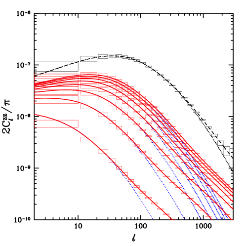
Figure 1.: The shear-shear auto power spectra. The 8 solid curves are the shear power spectra from each of the galaxy source planes, $B_{1}$ to $B_{8}$. Dotted curves are the linear perturbation theory approximation. From bottom to top the source plane redshift ranges are $B_{1}$: $z\in[0.0,0.4]$, $B_{2}$: $z\in[0.4,0.8]$, $B_{3}$: $z\in[0.8,1.2]$, $B_{4}$: $z\in[1.2,1.6]$, $B_{5}$: $z\in[1.6,2.0]$, $B_{6}$: $z\in[2.0,2.4]$, $B_{7}$: $z\in[2.4,2.8]$ and $B_{8}$: $z\in[2.8,3.2]$. The error boxes are forecasts for G4$\pi$ (see Table I). The top dashed curve is the shear power spectrum for the CMB source plane. The error boxes are forecasts for CMBpol.

2.2. Supernova Data Model

For the supernova survey we assume 2000 distributed in redshift as described in Kim et al. (2004) as a baseline SNAP supernova survey. In addition, we assume measurement of 100 local supernovae. To our parameter set, detailed above, we add a supernova luminosity calibration parameter. We do not explicitly include systematic errors in our analysis. The supernova forecasts in some sense do include systematic error estimates, because the SNAP baseline survey, by design, does not attempt to reduce statistical errors far below the expected systematic error limits (by intentionally restricting the number of supernovae in each redshift interval).

3. Constraints on $w_{0}$ and $w_{a}$

For dark energy models with sound speeds near unity, the Jeans scale is on the horizon and we can ignore clustering of the dark energy on scales smaller than the horizon, and certainly at $l<40$, the lowest $l$ value we consider. Thus the dark energy results in a time-dependent but scale-independent suppression of power. However, the scale-independence in three dimensions does not translate into a scale-independence of the two-dimensional projection to shear power spectra because the projection folds the time and scale-dependence together. Note though that in the special case of a power-law power spectrum the projection does preserve the scale-dependence. Thus, in the left panel of Figure 2 we see changing $w$ changes the shape of the power spectra, but not at small scales where the three-dimensional power spectrum is well–approximated as a power law. In addition to altering the growth rate, dark energy alters the shear power spectra by changing $D_{A}(z)$ and therefore the projection of the fluctuation power at different redshifts onto the sky.

The trend with redshift in the left panel of Figure 2 can be understood as arising from the dependence of the growth rate on $w_{0}$. Recall that we are changing $w_{0}$ while keeping the angular size of the sound horizon on the last-scattering surface (and hence the angular-diameter distance to last-scattering) fixed. Increasing $w_{0}$ from $w_{0}=-1$ means more dark energy at high redshift (since the dark energy density is now increasing with redshift as opposed to being constant) and less dark energy at low redshift (in order to keep the angular-diameter distance fixed). Thus, growth is suppressed at high redshift and enhanced at low redshift.

The scale-dependence of the shear power spectra dependence on the dark energy is a boon. The scale-dependence prevents the dark energy effects from being completely degenerate with a redshift-dependent calibration error. We have ignored shear calibration uncertainty in our analysis. It would be interesting to include it (as in Ishak et al. (2004)) and see how effectively the dataset can simultaneously constrain calibration and cosmological parameters, just with the assumption that the calibration is scale-independent.

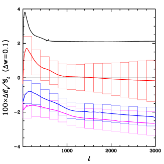
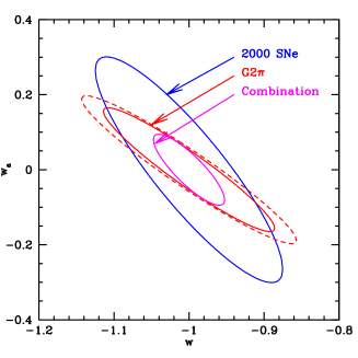
Figure 2.: Left panel shows difference between $w=-.9$ and $w=-1$ shear power spectra for source bins centered at $z=0.2$, $0.6$, $1.4$ and $3.0$ from top to bottom. The $z=0.2$ curve has no error bars on it because their large extent would clutter the graph. The right panel shows one $\sigma$ error contours in the $w_{0}$-$w_{a}$ plane for G$2\pi$, 2000 SNe and the combination (as labeled). The dashed curve is for G$2\pi$ with the source density uniformly decreased by a factor of 2.

The supernova data constrain the dark energy through the dependence of the luminosity distance (equivalent to $D_{A}(z)$ in a flat Universe) on the dark energy. The resulting constraint from the 2000 supernovae are also shown in Fig. 2. We see that the two error ellipses are not perfectly aligned. Combining the datasets results in a factor of 2 decrease in the $w_{a}$ direction and a factor of 3 decrease in the $w_{0}$ direction.

An advantage of using only the large angular scale statistics is their robustness to increases in shape noise. At $l<1000$, for most of the source redshift bins, the G$2\pi$ shear errors are dominated by sample variance not shape noise variance. Thus an increase in the shape noise variance by a factor of 2 for all source bins (as would happen if the source density were uniformly lower than expected by a factor of two) only leads to a small increase in the error contours, as shown with the dashed contours in Figure 2.

4. Constraints on higher-dimensional parameterizations

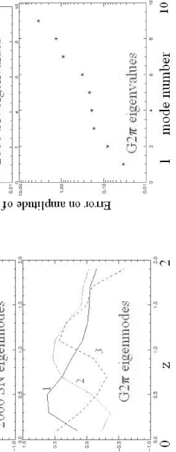
Figure 3.: Eigenvalues (right) and first three eigenmodes (left) of the $w(z)$ error covariance matrix for G$2\pi$+Planck and 2000 SNe+Planck. The large contributions to the eigenmodes from the highest redshift-bin are an artifact of that bin being much broader than the rest, extending all the way to the last-scattering surface.

To deepen our understanding of how these surveys are constraining dark energy, we have examined how they constrain the function $w(z)$, rather than its simple parameterization by $w_{0}$ and $w_{a}$. We proceed by binning $w(z)$ in redshift bins and then identifying the eigenmodes and eigenvalues of the binned $w(z)$ error covariance matrix as was done for supernovae by Huterer & Starkman (2003).

In the left panels of Figure 3 we plot the three eigenmodes with the best determined eigenvalues. We see a striking difference in the modes for 2000 SNe vs. the modes for G$2\pi$: those for G$2\pi$ stretch out to higher redshifts. The reason for this is that lensing is less sensitive to the growth factor at the lower redshifts where the source density in a given redshift bin is small and the lensing window (for sources at higher redshift) is also small. Thus the supernovae are better at detecting changes in $w(z)$ at lower redshift and G$2\pi$ tends to be better at detecting changes at higher redshift.

G$2\pi$ and 2000 SNe also have strikingly different eigenvalue spectra. The error on the amplitude of the best determined mode is quite similar for each ($\sim 0.03$). But the 2000 SNe spectrum is much steeper. G$2\pi$ has seven modes with errors smaller than unity, whereas 2000 SNe has four.

To further explore the power of these experiments to constrain dark energy we chose eigenmodes of $w(z)$ because it was calculationally convenient for us. There are probably parameterizations with superior qualities. One we have begun exploring is modes of $\rho_{d.e.}(z)$, with the constraint that one of the modes is constant; i.e., independent of $z$. This approach has two virtues. First, the density is more directly related to the data than the equation-of-state parameter. Second, interpretation of data as evidence for non-cosmological-constant behavior is straightforward; one only need assess how significantly non-zero the amplitudes of the non-constant modes are.

5. Conclusions

As we have seen from Bernstein’s talk and Jain’s talk, weak lensing datasets are very rich, with dark energy constraints possible from a variety of statistical measures. Here we have studied just one statistic, the shear-shear two-point functions on large angular scales. Even restricting ourselves in this manner, we find the potential power of large-area weak lensing surveys is extraordinary. Further, we see that the statistical weight of the data constrain directions in parameter space different from those constrained by supernovae; i.e., they are complementary. Therefore the combination is particularly powerful.

To more fully understand how these different observations probe dark energy we examined eigenmodes of the $w(z)$ error covariance matrix. We saw that the G$2\pi$ observations are better at probing $w(z)$ at high redshift and the supernova observations are better at lower redshifts. A handful of eigenmodes could be determined with less than 100% errors.

This work has illustrated the different statistical uncertainties on dark energy parameters for two types of probes. A side by side comparison of comprehensive error forecasts is a much more ambitious undertaking that would require detailed consideration of systematic errors and the extent to which they can be controlled.

Acknowledgments.

We thank B. Gold, M. Kaplinghat, E. Linder, S. Perlmutter, U. Seljak and T. Tyson for useful conversations and the organizers for a stimulating meeting. This material is based upon work supported by the DoE, NASA grant NAG5-11098 and by NSF grant 0307961.

References

- Bennett et al. (2003) Bennett, C. L., Halpern, M., Hinshaw, G., Jarosik, N., Kogut, A., Limon, M., Meyer, S. S., Page, L., Spergel, D. N., Tucker, G. S., Wollack, E., Wright, E. L., Barnes, C., Greason, M. R., Hill, R. S., Komatsu, E., Nolta, M. R., Odegard, N., Peiris, H. V., Verde, L., & Weiland, J. L. 2003, ApJS, 148, 1
- Bernstein & Jain (2004) Bernstein, G. & Jain, B. 2004, ApJ, 600, 17
- Hu & Jain (2003) Hu, W. & Jain, B. 2003, ArXiv Astrophysics e-prints
- Huterer & Starkman (2003) Huterer, D. & Starkman, G. 2003, Physical Review Letters, 90, 31301
- Ishak et al. (2004) Ishak, M., Hirata, C. M., McDonald, P., & Seljak, U. 2004, Phys.Rev.D, 69, 083514
- Jain & Taylor (2003) Jain, B. & Taylor, A. 2003, Physical Review Letters, 91, 141302
- Kaplinghat et al. (2003) Kaplinghat, M., Knox, L., & Song, Y. 2003, ArXiv Astrophysics e-prints, 3344
- Kim et al. (2004) Kim, A. G., Linder, E. V., Miquel, R., & Mostek, N. 2004, MNRAS, 347, 909
- Nagashima et al. (2002) Nagashima, M., Yoshii, Y., Totani, T., & Gouda, N. 2002, ArXiv Astrophysics e-prints, 7483
- Refregier et al. (2003) Refregier, A., Massey, R., Rhodes, J., Ellis, R., Albert, J., Bacon, D., Bernstein, G., McKay, T., & Perlmutter, S. 2003, ArXiv Astrophysics e-prints
- Song & Knox (2003) Song, Y. & Knox, L. 2003, ArXiv Astrophysics e-prints
- Takada & Jain (2003) Takada, M. & Jain, B. 2003, ArXiv Astrophysics e-prints
- Takada & White (2003) Takada, M. & White, M. 2003, ArXiv Astrophysics e-prints
- Tauber (2001) Tauber, J. A. 2001, in IAU Symposium, 493–+
- Tyson et al. (2003) Tyson, J. A., Wittman, D. M., Hennawi, J. F., & Spergel, D. N. 2003, astro-ph/0209632. Nuc. Phys. B, 124, 21