Correspondence between the adhesion model and the velocity dispersion for the cosmological fluid

Abstract

Basing our discussion on the Lagrangian description of hydrodynamics, we studied the evolution of density fluctuation for nonlinear cosmological dynamics. Adhesion approximation (AA) is known as a phenomenological model that describes the nonlinear evolution of density fluctuation rather well and that does not form a caustic. In addition to this model, we have benefited from discussion of the relation between artificial viscosity in AA and velocity dispersion. Moreover, we found it useful to regard whether the velocity dispersion is isotropic produces effective ‘pressure’ or viscosity terms. In this paper, we analyze plane- and spherical-symmetric cases and compare AA with Lagrangian models where pressure is given by a polytropic equation of state. From our analyses, the pressure model undergoes evolution similar to that of AA until reaching a quasi-nonlinear regime. Compared with the results of a numerical calculation, the linear approximation of the pressure model seems rather good until a quasi-nonlinear regime develops. However, because of oscillation arising from the Jeans instability, we could not produce a stable nonlinear structure.

I Introduction

The Lagrangian description for the cosmological fluid can be usefully applied to the structure formation scenario. This description provides a relatively accurate model even in a quasi-linear regime. Zel’dovich zel proposed a linear Lagrangian approximation for dust fluid. This approximation is called the Zel’dovich approximation (ZA) zel ; Arnold82 ; Shandarin89 ; buchert89 ; coles ; saco . ZA describes the evolution of density fluctuation better than the Eulerian approximation munshi ; sahsha ; yoshisato . Although ZA gives an accurate description until a quasi-linear regime develops, ZA cannot describe the model after the formation of caustics. In ZA, even after the formation of caustics, the fluid elements keep moving in the direction set up by the initial condition. Therefore, the nonlinear structure that it is formed diffuses at once, while N-body simulation shows the presence of a dense structure with a very wide range in mass at any given time davis .

In order to proceed with a hydrodynamical description in which caustics do not form, the ‘adhesion approximation’ gurbatov (AA) was proposed based on the model equation of nonlinear diffusion (Burgers’ equation). In AA, an artificial viscosity term is added to ZA. Because of the viscosity term, we can avoid caustics formation. From the standpoint of AA, the problem of structure formation has been discussed Shandarin89 ; weinberg90 ; nusser ; kofman ; msw . The density divergence does not occur in AA, and the density distribution close to the N-body simulation can be produced. However, the origin of the viscosity has not yet been clarified.

Buchert and Domínguez budo discussed the effect of velocity dispersion using the collisionless Boltzmann equation BT . They argued that models of a large-scale structure should be constructed for a flow describing the average motion of a multi-stream system. Then they showed that when the velocity dispersion is regarded as small and isotropic it produces effective ‘pressure’ or viscosity terms. Furthermore, they posited the relation between mass density $\rho$ and pressure $P$, i.e., an ‘equation of state’. Buchert et al. bdp showed how the viscosity term or the effective pressure of a fluid is generated, assuming that the peculiar acceleration is parallel to the peculiar velocity. Domínguez domi00 ; domi0106 clarified that a hydrodynamic formulation is obtained via a spatial coarse-graining in a many-body gravitating system, and that the viscosity term in AA can be derived by the expansion of coarse-grained equations.

With respect to the relation between the viscosity term and effective pressure, and the extension of the Lagrangian description to various matter, the Lagrangian perturbation theory of pressure has been considered. Actually, Adler and Buchert adler have formulated the Lagrangian perturbation theory for a barotropic fluid. Morita and Tatekawa moritate and Tatekawa et al. tate02 solved the Lagrangian perturbation equations for a polytropic fluid up to the second order. Hereafter, we call this model the ‘pressure model’.

In this paper, we analyze the evolution of the density fluctuation in several Lagrangian models using simple models. From these analyses, we examine the following questions. (a) Can we explain the origin of the viscosity term in AA with ‘pressure’? (b) How long is the linear approximation of the pressure model valid? (c) Can we avoid the formation of a caustic with the pressure model? To answer these questions, we analyze time evolution for plane- and spherical-symmetric cases with first- (ZA), second- (PZA), and third-order approximation (PPZA), and for the exact solution for dust fluid, AA, and the pressure model (linear approximation and full-order). As shown by previous papers moritate ; tate02 ; tate04 , the behavior of the pressure model strongly depends on the polytropic exponent $\gamma$. By the fine tuning of the parameter, the pressure model can reproduce time evolution similar to that of AA until a quasi-nonlinear regime develops. Furthermore, until the development of a quasi-nonlinear regime, the linear approximation of the pressure model seems rather good when compared with a full-order numerical calculation. However, the tendencies change greatly in a nonlinear regime. Because of the Jeans instability, in the pressure model, the density fluctuation oscillates. This oscillation of the fluctuation appears in both the linear approximation and the full-order calculation. Because the oscillation of the fluctuation does not occur in AA, the pressure model cannot reproduce the behavior of AA completely. Of course, as in the case of the dust fluid, the linear approximation of the pressure model becomes worse in the nonlinear regime.

The behavior of the fluctuation after the oscillation strongly depends on the parameters. In a previous paper tate04 , although the case where $\gamma=5/3$ showed a rather good result when compared with N-body simulation, caustics formation could not be avoided. Where $\gamma=4/3$, the result seemed to resemble that of AA. However, in a long-duration evolution of the pressure model, even if a full-order equation was considered, caustics formed. Where $\gamma=1$, the fluctuation disappeared. Although behavior similar to AA can be discussed with the pressure model until a quasi-nonlinear regime develops, more consideration is necessary to ascertain the existence of a stable nonlinear structure.

From our analyses, we conclude that we cannot sufficiently explain the origin of the viscosity term in AA with the pressure model. This conclusion does show, however, that we should apply the pressure model in other situations. Recently, various dark matter models have been proposed DarkMatter . Some of them affect not only the gravity but also a special interaction. We also show that the linear approximation of the pressure model seems rather good until a quasi-linear regime develops. If the interactions of the dark matter are affected by effective pressure, the linear approximation can be applied for the analysis of the quasi-nonlinear evolution of the density fluctuation.

This paper is organized as follows. In Sec. II, we present Lagrangian perturbative solutions in the Einstein-de Sitter (E-dS) universe. In Sec. II.1, we show perturbative solutions for dust fluid up to a third-order approximation. Here we consider only the longitudinal mode. In Sec. II.2, we mention the problem of ZA and show the solution of AA. In Sec. II.3, we explain the pressure model.

In Sec. III, we compare the evolution of the density fluctuation between the Lagrangian approximations. In Sec. III.1, we analyze the plane-symmetric case. Here ZA gives the exact solution for dust fluid. In order to show the special tendency of this solution, we analyze the spherical-symmetric case in Sec. III.2. In Sec. IV, we discuss our results and state our conclusions.

II The Lagrangian description for the cosmological fluid

In this section, we present perturbative solutions in the Lagrangian description. In Lagrangian hydrodynamics, the comoving coordinates $\bm{x}$ of the fluid elements are represented in terms of Lagrangian coordinates $\bm{q}$ as

$$\bm{x}=\bm{q}+\bm{s}(\bm{q},t)\,,$$ (1)

where $\bm{s}$ denotes the Lagrangian displacement vector due to the presence of inhomogeneities. From the Jacobian of the coordinate transformation from $\bm{x}$ to $\bm{q}$, $J\equiv\det(\partial x_{i}/\partial q_{j})=\det(\delta_{ij}+\partial s_{i}/\partial q_{j})$, the mass density is described exactly as

$$\rho=\rho_{\rm b}J^{-1}\,,$$ (2)

where $\rho_{\rm b}$ means background average density.

We decompose $\bm{s}$ into the longitudinal and the transverse modes as $\bm{s}=\nabla_{\bm{q}}S+\bm{S}^{\rm T}$ with $\nabla_{\bm{q}}\cdot\bm{S}^{\rm T}=0$. In this paper, we show an explicit form of perturbative solutions only in the Einstein-de Sitter (E-dS) universe.

II.1 The Lagrangian perturbation for dust fluid

Zel’dovich derived a first-order solution of the longitudinal mode for dust fluid zel . For the E-dS model, the solutions are written as follows:

$$S^{(1)}(\bm{q},t)=t^{2/3}S_{+}(\bm{q})+t^{-1}S_{-}(\bm{q})\,.$$ (3)

This first-order approximation is called the Zel’dovich approximation (ZA). Especially when we consider the plane-symmetric case, ZA gives exact solutions Arnold82 .

ZA solutions are known as perturbative solutions, which describe the structure well in the quasi-nonlinear regime. To improve approximation, higher-order perturbative solutions of Lagrangian displacement were derived. Irrotational second-order solutions (PZA) were derived by Bouchet et al. bouchet92 and Buchert and Ehlers bueh93 , and third-order solutions (PPZA) were obtained by Buchert buchert94 , Bouchet et al. bouchet95 , and Catelan catelan . The second-order and third-order solutions are written as follows:

$$S^{(2)}_{i,i} = \frac{3}{14}\left(S^{(1)}_{i,j}S^{(1)}_{j,i}-S^{(1)}_{i,i}S^{(1)}_{j,j}\right)\,,$$ (4)

$$S^{(3)}_{i,i} = \frac{5}{9}\left(S^{(1)}_{i,j}S^{(2)}_{j,i}-S^{(1)}_{i,i}S^{(2)}_{j,j}\right)-\frac{1}{3}\mbox{det}\left(S^{(1)}_{i,j}\right)\,,$$ (5)

where the superscript $S^{(n)}$ means n-th order solutions.

Though third-order solutions have been obtained for the transverse mode buchert92 ; sasakasa , because we consider only longitudinal modes, we will pass over those details here.

II.2 Adhesion approximation

Cosmological N-body simulations show that pancakes, skeletons, and clumps remain during evolution. However, when we continue applying the solutions of ZA, PZA, or PPZA after the appearance of caustics, the nonlinear structure diffuses and breaks.

Adhesion approximation (AA) gurbatov was proposed from a consideration based on Burgers’ equation. This model is derived by the addition of an artificial viscous term to ZA. AA with small viscosity deals with the skeleton of the structure, which at an arbitrary time is found directly without a long numerical calculation.

We briefly describe the adhesion model. In ZA, the equation for ‘peculiar velocity’ in the E-dS model is written as follows:

$$\frac{\partial\bm{u}}{\partial a}+(\bm{u}\cdot\nabla_{x})\bm{u} = 0\,,$$ (6)

$$\bm{u}\equiv\frac{\partial\bm{x}}{\partial a}=\frac{\dot{\bm{x}}}{\dot{a}}\,,$$ (7)

where $a(\propto t^{2/3})$ means scale factor. To go beyond ZA, we add the artificial viscosity term to the right side of the equation.

$$\frac{\partial\bm{u}}{\partial a}+(\bm{u}\cdot\nabla_{x})\bm{u}=\nu\nabla_{x}^{2}\bm{u}\,.$$ (8)

We consider the case when the viscosity coefficient $\nu\rightarrow+0$ ($\nu\neq 0$). In this case, the viscosity term especially affects the high-density region. Within the limits of a small $\nu$, the analytic solution of Eq.(8) is given by

$$\bm{u}(\bm{x},t)=\sum_{\alpha}\left(\frac{\bm{x}-\bm{q}_{\alpha}}{a}\right)j_{\alpha}\exp\left(-\frac{I_{\alpha}}{2\nu}\right)/\sum_{\alpha}j_{\alpha}\exp\left(-\frac{I_{\alpha}}{2\nu}\right)\,,$$ (9)

where $\bm{q}_{\alpha}$ means the Lagrangian points that minimize the action

$$I_{\alpha} \equiv I(\bm{x},a;\bm{q}_{\alpha})=S_{0}(\bm{q}_{\alpha})+\frac{(\bm{x}-\bm{q}_{\alpha})^{2}}{2a}=\mbox{min.}\,,$$ (10)

$$j_{\alpha} \equiv \left.\left[\det\left(\delta_{ij}+\frac{\partial^{2}S_{0}}{\partial q_{i}\partial q_{j}}\right)\right]^{-1/2}\right|_{\bm{q}=\bm{q}_{\alpha}}\,,$$ (11)

$$S_{0} = S(\bm{q},t_{0})\,,$$ (12)

considered as a function of $\bm{q}$ for fixed $\bm{x}$ kofman . In AA, because of the viscosity term, the caustic does not appear and a stable nonlinear structure can exist.

II.3 Pressure model

Although AA seems a good model for avoiding the formation of caustics, the origin of the modification (or artificial viscosity) is not clarified. Buchert and Domínguez budo argued that the effect of velocity dispersion becomes important beyond the caustics. They showed that when the velocity dispersion is still small and can be considered isotropic, it gives effective ‘pressure’ or viscosity terms. Buchert et al. bdp showed how the viscosity term is generated by the effective pressure of a fluid under the assumption that the peculiar acceleration is parallel to the peculiar velocity.

Adler and Buchert adler have formulated the Lagrangian perturbation theory for a barotropic fluid. Morita and Tatekawa moritate and Tatekawa et al. tate02 solved the Lagrangian perturbation equations for a polytropic fluid in the Friedmann Universe. Hereafter, we call this model the ‘pressure model’.

When we consider the polytropic equation of state $P=\kappa\rho^{\gamma}$, the first-order solutions for the longitudinal mode are written as follows. For $\gamma\neq 4/3$,

$$\widehat{S}(\bm{K},a)\propto a^{-1/4}\,\mathcal{J}_{\pm 5/(8-6\gamma)}\left(\sqrt{\frac{2C_{2}}{C_{1}}}\frac{|\bm{K}|}{|4-3\gamma|}\,a^{(4-3\gamma)/2}\right)\,,$$ (13)

where $\mathcal{J}_{\nu}$ denotes the Bessel function of order $\nu$, and for $\gamma=4/3$,

$$\widehat{S}(\bm{K},a)\propto a^{-1/4\pm\sqrt{25/16-C_{2}|\bm{K}|^{2}/2C_{1}}}\,,$$ (14)

where $C_{1}\equiv 4\pi G\rho_{\rm b}(a_{\rm in})\,a_{\rm in}^{\ 3}/3$ and $C_{2}\equiv\kappa\gamma\rho_{\rm b}(a_{\rm in})^{\gamma-1}\,a_{\rm in}^{\ 3(\gamma-1)}$. $\rho_{b}$ and $\bm{K}$ mean background mass density and Lagrangian wavenumber, respectively. $a_{\rm in}$ means scale factor when an initial condition is given. When we take the limit $\kappa\rightarrow 0$, these solutions agree with Eq. (3).

In this model, the behavior of the solutions strongly depends on the relation between the scale of fluctuation and the Jeans scale. Here we define the Jeans wavenumber as

$$K_{\rm J}\equiv\left(\frac{4\pi G\rho_{\rm b}a^{2}}{{\rm d}P/{\rm d}\rho(\rho_{\rm b})}\right)^{1/2}\,.$$

The Jeans wavenumber, which gives a criterion for whether a density perturbation with a wavenumber will grow or decay with oscillation, depends on time in general. If the polytropic index $\gamma$ is smaller than $4/3$, all modes become decaying modes and the fluctuation will disappear. On the other hand, if $\gamma>4/3$, all density perturbations will grow to collapse. In the case where $\gamma=4/3$, the growing and decaying modes coexist at all times.

We rewrite the first-order solution Eq. (13) with the Jeans wavenumber:

$$\widehat{S}(\bm{K},a)\propto a^{-1/4}\,\mathcal{J}_{\pm 5/(8-6\gamma)}\left(\frac{\sqrt{6}}{|4-3\gamma|}\frac{|\bm{K}|}{K_{\rm J}}\right)\,.$$ (15)

In this paper, we analyze the first-order perturbation and the full-order solution. The evolution equation for the longitudinal mode is written as follows  adler ; moritate :

$$\nabla_{x}\cdot\left(\nabla_{q}\ddot{\bm{s}}+2\frac{\dot{a}}{a}\nabla_{q}\dot{\bm{s}}-\frac{\kappa\gamma\rho_{b}^{\gamma-1}}{a^{2}}J^{-\gamma}\nabla_{x}J\right)=-4\pi G\rho_{b}(J^{-1}-1)\,.$$ (16)

In general, it is very difficult to solve this equation for such reasons as the coordinate transformation or non-locality. Here, we imposed symmetry and avoided these difficulties.

III Comparison between Lagrangian models

III.1 The plane-symmetric case

First, we analyze the plane-symmetric case. In the plane-symmetric case, ZA gives exact solutions for dust fluid. However, when we keep using the solutions of ZA after the appearance of caustics, the nonlinear structure diffuses and breaks. We must connect the solutions with several procedures to continue the calculation after the formation of caustics.

To simplify, we treat the single-wave case.

$$S_{0}(q)=\varepsilon\cos q\,.$$ (17)

The initial peculiar velocity is made equal with that given by the growing mode in ZA. The evolution of this model for ZA, AA, and N-body simulation (extrapolation of ZA) was analyzed by Nusser and Dekel nusser . In this calculation, we set up the normalization of the scale factor when first caustics appear with ZA by a=1. At a late time, the caustics will diffuse in ZA. AA remains a high-density filament and caustics do not appear.

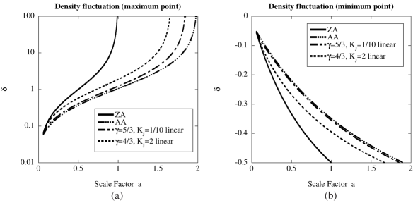
Figure 1: The evolution of density in linear approximations (ZA, AA, and the pressure model). The viscosity parameter in AA is given by $\nu=(\pi/512)^{2}$. (a) The density of the densest point. In AA, the density remains finite forever. On the other hand, in the pressure model, if $\gamma>4/3$, the density becomes infinity. Therefore, we cannot avoid the formation of the caustic. (b) The density of the sparsest point. The growth of the void with the pressure model is fast in comparison with AA.

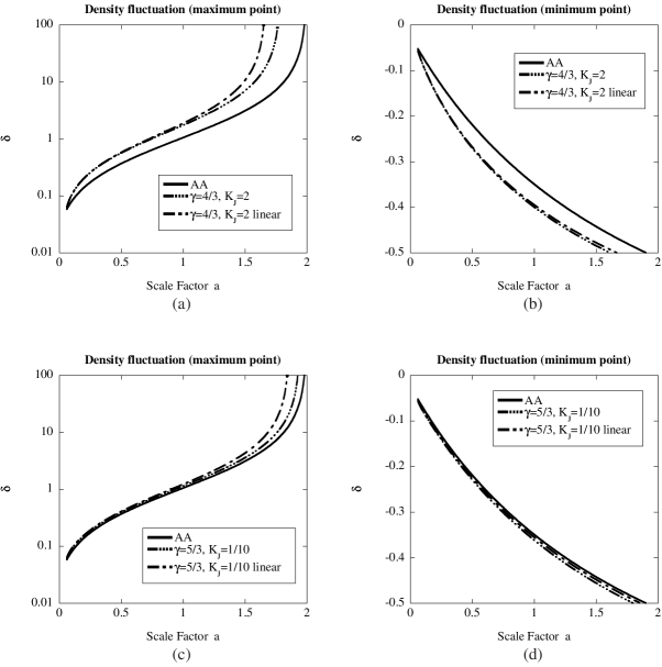
Figure 2: The evolution of density in AA and the pressure model (linear approximation and full-order). In the pressure model, the nonlinear effect suppresses the evolution of density fluctuation. Therefore,the linear approximation becomes worse in a strongly nonlinear regime. If $\gamma>4/3$, although we calculate a full-order model, we cannot avoid the formation of the caustic. (a) The case where $\gamma=4/3$, the density of the densest point. (b) The case where $\gamma=4/3$, the density of the sparsest point. (c) The case where $\gamma=5/3$, the density of the densest point. (d) The case where $\gamma=5/3$, the density of the sparsest point.

We analyze the time evolution of this model with the pressure models. As mentioned in the previous section, the relation between the Jeans scale and the scale of fluctuation is important for evolution in these models. We consider only the case in which the scale of fluctuation is larger than the initial Jeans scale. At first, we analyze the linear perturbation of the pressure model. In the linear perturbation, we consider the case where $\gamma=4/3,5/3$, because the fluctuation does not grow if $\gamma<4/3$.

Fig. 1 shows the evolution of density in ZA, AA, and the linear approximation of the pressure model. As with the viscosity in AA, the effect of the pressure delays the growth of the fluctuation. In the case where $\gamma=5/3$, because the perturbative solutions asymptotically become those of ZA, the fluctuation grows rapidly at once. In the case where $\gamma=4/3$, if we choose a reasonable value for $K_{\rm J}$, though growth of the fluctuation can be slowed, caustics are formed in the end (Fig. 1 (a)). In any case, though it seems that the behavior of AA can be almost reproduced with the pressure model by the fine-tuning of the parameter, because the linear perturbative solutions keep growing, the formation of the caustics cannot be prevented where $\gamma>4/3$. Therefore, the linear approximation of the pressure model cannot reproduce the behavior of AA completely. As for the region where the density fluctuation is negative (Fig. 1 (b)), in comparison with ZA, AA and the pressure model suppress the growth of the fluctuation.

Next we analyze the behavior of the solutions of the pressure model without the approximation (Fig. 2). Although the fluctuation keeps growing when we use the linear approximation, we expect that the growth of the fluctuation may be restrained by the effect of nonlinearity. In fact, in previous papers, we showed that the second-order perturbations suppress the growth of the fluctuation moritate ; tate02 .

Here we analyze the case where $\gamma=4/3,5/3$. In both cases, the difference between the linear approximation deviates from the full-order calculation greatly after $\delta>1$. In the case where $\gamma=4/3$ (Fig. 2 (a), (b)), though the behavior of the solution strongly depends on the relation between the scale of fluctuation and the Jeans scale, we can delay the formation of caustics drastically. However, when we analyze long-duration evolution, the density fluctuation eventually diverges and the caustics form. In the case where $\gamma=5/3$ (Fig. 2 (c), (d)), the growth of the fluctuation cannot be restrained considerably either, as in the second-order perturbation. Although good results were achieved in the comparison with the N-body simulation tate04 , it is difficult to restrain the formation of the caustics in the case where $\gamma=5/3$.

From these results, when $\gamma=4/3$, the growth of the fluctuation can be gentle. However the caustics are finally formed, the divergence of density cannot be avoided as with AA. In other words, in the plane-symmetric case, we cannot represent the behavior that resembles AA.

From Fig. 2, the linear approximation of the pressure model gives a rather good result until a quasi-nonlinear regime develops. In a strongly nonlinear regime, the growth of the density fluctuation in the linear approximation becomes slightly fast, because of linearized pressure.

Because the results in this subsection may depend on symmetry, we will analyze the spherical-symmetric case in the next subsection.

III.2 The spherical-symmetric case

For the spherical-symmetric case, dust collapse and void evolution have been analyzed munshi ; sahsha ; yoshisato . Here we consider the evolution with ZA, PZA, PPZA, the exact solution for dust fluid, AA, and the pressure models. To avoid a discontinuity of the pressure gradient, we adopt the Mexican-hat type model (Fig. 3):

$$\delta(r)=\varepsilon(3-r^{2})e^{-r^{2}/2}\,.$$ (18)

This model has several merits. For one the fluctuation is derived by the two times differential calculus of Gaussian

$$-\nabla^{2}\left(\varepsilon e^{-r^{2}/2}\right)=-\frac{1}{r^{2}}\frac{\partial}{\partial r}\left(r^{2}\frac{\partial}{\partial r}\left(\varepsilon e^{-r^{2}/2}\right)\right)=\varepsilon(3-r^{2})e^{-r^{2}/2}\,,$$ (19)

and the average of density fluctuation over the whole space becomes zero:

$$\int_{0}^{\infty}4\pi r^{2}\delta(r){\rm d}r=0\,.$$ (20)

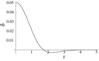
Figure 3: Mexican-hat type model. The average of density fluctuation over the whole space becomes zero.

The initial peculiar velocity is made equal with that of the growing mode in ZA. For this model, from Eq. (3)-(5), the solutions of ZA, PZA, and PPZA are given as follows:

$$S^{(1)} = -\varepsilon e^{-r^{2}/2}\,,$$ (21)

$$S^{(2)} = -\frac{3}{7}\varepsilon^{2}e^{-r^{2}}\,,$$ (22)

$$S^{(3)} = -\frac{46}{189}\varepsilon^{3}e^{-3r^{2}/2}\,.$$ (23)

In our analysis, we set the value of $\varepsilon$ as follows:

$$\varepsilon=\pm\frac{1}{60}\,.$$ (24)

Under this condition, the initial density fluctuation at $r=0$ becomes $\delta=\pm 0.05$. Then the scale factor is set as $a=0.0167(=1/60)$ at the initial condition. In the case where $\varepsilon>0$, the caustics appear at $a=1$ in ZA. The initial peculiar velocity is equal with that given by the growing mode in ZA.

In past analyses munshi ; sahsha ; yoshisato , homogeneous spherical collapse and void evolution have been analyzed. Here we consider spherical but inhomogeneous density fluctuation. We investigate time evolution in the dust model first because it may produce a result that differs from that of past analyses.

Fig. 4 shows the time evolution of the Mexican-hat type density fluctuation in the dust model. For spherical collapse, as well as in the past analyses, when we considered higher order perturbation, the occurrence time of the caustics becomes fast munshi ; sahsha ; yoshisato . The caustic appears with an exact solution at $a\simeq 0.55$. On the other hand, the growth of the fluctuation becomes gentle, and the caustic does not appear in AA. For void evolution, the evolution of the density fluctuation stops gradually with PZA, and it starts to proceed in reverse. When we consider long-time evolution, PPZA deviates from an exact solution greatly more than ZA does. These results correspond to past analyses considering homogeneous spherical distribution.

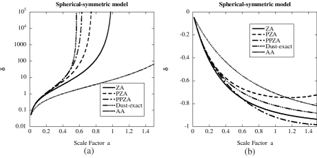
Figure 4: The evolution of the spherical-symmetric (the Mexican-hat type) density fluctuation at $r=0$ in dust models. (a) The evolution of a density fluctuation in ZA, PZA, PPZA, the exact model, and AA in the case where $\varepsilon>0$. The viscosity parameter in AA is set as $\nu=(1/512)^{2}$. The approximation is improved by higher order perturbation. In the exact model, the caustic appears at $a\simeq 0.55$. On the other hand, the density fluctuation evolves gently in AA. (b) The same as (a) but the case where $\varepsilon<0$. In PZA, the fluctuation becomes positive during evolution. Later ($a>0.6$), PPZA deviates from an exact solution greatly more than ZA does.

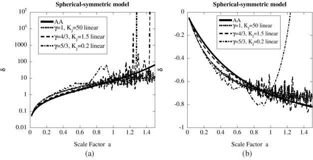
Figure 5: The evolution of the spherical-symmetric (Mexican-hat type) density fluctuation at $r=0$ in the pressure models with the linear approximation. (a) The evolution of a density fluctuation in the case where $\varepsilon>0$. Until a quasi-nonlinear regime develops, the pressure models show behavior resembling AA. However, the fluctuation oscillates in the nonlinear region. In the case where $\gamma=1$, the fluctuation oscillates little by little. Finally the fluctuation decays and disappears. In the case where $\gamma=4/3$, the fluctuation oscillates and the caustic appears at $a\simeq 1.44$. In the case where $\gamma=5/3$, the oscillation of the fluctuation in the intermediate state grows very large. Then the caustic appears at $a\simeq 1.28$. (b) The same as (a) but here $\varepsilon<0$. In the case where $\gamma=1$, finally the fluctuation decays and disappears. In the case where $\gamma=4/3$, although the fluctuation oscillates, the density asymptotically decreases. In the case where $\gamma=5/3$, the density fluctuation becomes positive during evolution because the oscillation of the fluctuation grows very large.

Next, we show how the Mexican-hat type fluctuation evolves in the pressure model. Fig. 5 shows the evolution of the Mexican-hat type fluctuation in the pressure model with linear approximation. Fig. 5 (a) shows spherical collapse in the pressure models. In the pressure model with linear approximation, the evolution of the fluctuation shows strange behavior. In the plane-symmetric case, the fluctuation includes only the single wave mode. On the other hand, in the spherical-symmetric case, the fluctuation includes various modes. Because of the difference of the growth rate between the various modes, the time evolution of the fluctuation does not become monotonous. At first, because we set the initial velocity in the direction in which the fluctuation grows, the fluctuation grows gently. Then, under the effect of pressure, the fluctuation begins to oscillate. Finally, the fluctuation grows or decays. The final state of the evolution strongly depends on the value of $\gamma$.

Here we adjust the value of $\kappa$, i.e., $K_{\rm J}$ in the pressure models, to elicit behavior resembling a case of AA. For the case where $\gamma=1$, when we consider the case of a small Jeans scale, the fluctuation grows in the early stage. After that, the fluctuation oscillates little by little. Finally, the fluctuation decays. For the case where $\gamma=4/3$, as well as the plane-symmetric case, the behavior depends on the relation between the Jeans scale and the scale of the structure. In linear approximation, when the scale of the structure is larger than the Jeans scale, because the perturbative solution produces the growing mode, the structure will collapse and form caustics. In our analysis, when we choose $K_{\rm J}=1.5$, the fluctuation oscillates and diverges. The behavior of the fluctuation strongly depends on the value of $K_{\rm J}$. Furthermore, relative to the growth rate of the fluctuation, the time of the formation of caustics varies greatly over a few differing values of $K_{\rm J}$. For the case where $\gamma=5/3$, the oscillation of the fluctuation in the intermediate state grows very large. Then the caustic is formed.

Fig. 5 (b) shows the void evolution in the pressure models. As well as in the spherical collapse case, the evolution of the fluctuation shows strange behavior. When the fluctuation grows to $\delta\simeq-0.5$, it begins to oscillate. Finally, the fluctuation grows or decays. Especially, in the case where $\gamma=5/3$, the fluctuation shows unrealistic evolution; the density fluctuation becomes positive during evolution, because the oscillation of the fluctuation grows very large.

When the fluctuation grew very large, we found that the behavior of AA could not be reproduced any more in the pressure model with linear approximation. In other words, it is very difficult to explain the origin of the viscosity term in AA by the pressure model. The oscillation of the fluctuation in the pressure model with linear approximation is caused by the Jeans instability. We will mention details about this oscillatory period and the amplitude in Sec. IV.

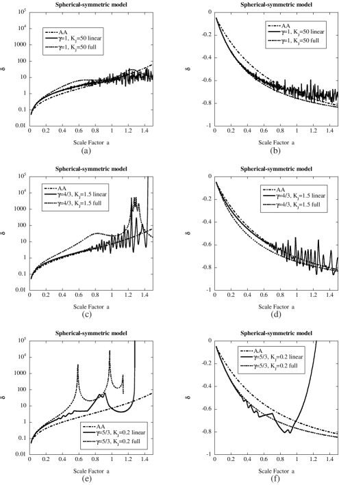
Figure 6: The evolution of a density fluctuation at $r=0$ in the spherical-symmetric case. These figures show the evolution in AA and the pressure models (linear approximation and the full-order calculation). These figures show the case where $\varepsilon>0$. (a) In the case where $\varepsilon>0$ and $\gamma=1$. In the pressure model, linear approximation seems valid until $\delta\simeq 1$. After that, in linear approximation, the fluctuation oscillates violently. In a strongly nonlinear region ($\delta>10$), even if we consider full-order calculation in the pressure model, the evolution of a fluctuation similar to AA cannot be reproduced. (b) The same as (a), but here $\varepsilon<0$. As in the case where $\varepsilon>0$, when the fluctuation evolve fully ($\delta<-0.5$), the fluctuation begins to oscillate. Finally the fluctuation decays and approaches to $0$. (c) The same as (a), but here $\gamma=4/3$. In the pressure model with linear approximation, the fluctuation oscillates, and the caustic appears at $a\simeq 1.44$. When we consider a full-order equation, although we can delay the density divergence, we cannot avoid the formation of the caustic. (d) The same as (b), but here $\gamma=4/3$. In the linear approximation in the pressure model, although the fluctuation oscillates, the density asymptotically decreases. In the pressure model, when we consider a full-order calculation, we can realize the evolution of a fluctuation similar to that of AA. (e) The same as (a), but here $\gamma=5/3$. In the pressure model with the linear approximation, the oscillation of the fluctuation in the intermediate state grows very large. Then the caustic appears at $a\simeq 1.28$. When we consider a full-order equation, the density diverges a little to the outside at $a\simeq 1.14$, and the model fails. (f) The same as (b), but here $\gamma=5/3$. In the linear approximation in the pressure model, the density fluctuation becomes positive during evolution because the oscillation of the fluctuation grows very large. On the other hand, when we consider a full-order equation, it is different from linear approximation, the density fluctuation always remaining negative.

When we solve the equation without approximation (Eq. (16)), how does the behavior of the density fluctuation change? These results are shown in Fig. 6. When we solve Eq. (16) for spherical collapse ($\varepsilon>0$) cases, such strange behavior as violent oscillation is suppressed, and the evolution of the fluctuation becomes smooth. However, these cases are different from the plane-symmetric case; if pressure is ignored in the spherical-symmetric case, the gravity term contains non-linear terms. Therefore, when we consider a full-order calculation, the contribution of not only the pressure but also the gravity becomes strong. Then if we choose a small value for $K_{J}$, the fluctuation sometimes grows earlier than in the case of linear approximation (Fig. 6 (a), (c), and (e)). In either case, the general tendency of the evolution of the fluctuation does not differ very much. According to Fig. 6 (a), (c), and (e), linear approximation of the pressure model seems to good until the quasi-nonlinear regime develops. The final state is unchanged, though a few differences are seen in the growth of the fluctuation, oscillatory amplitude, and period. In other words, even if the full-order calculation is considered, it is very difficult to explain the origin of the viscosity term in AA by the pressure model.

Next, we mention the evolution of a void (the case where $\varepsilon<0$). When we consider a full-order calculation, unrealistic behavior, such as linear approximation in the case where $\gamma=5/3$ (Fig. 5 (b)), does not appear. Furthermore, the oscillation of the fluctuation is suppressed, and the growth of the fluctuation comes to look like that of AA. In the evolution of the void, the linear approximation of the pressure model seems good until $\delta\simeq-0.5$. When we do not introduce linear approximation, the oscillation of the density fluctuation is almost imperceptible (Fig. 6 (b), (d), and (f)).

Although we can realize a void evolution in AA with the pressure model, we cannot reproduce the existence of a stable nonlinear structure. In other words, it is very difficult to find the origin of artificial viscosity in AA with the isotropic velocity dispersion.

According to our calculation in linear approximation, the amplitude and the period of the oscillation of the fluctuation in the intermediate state obviously depends on $\gamma$. Although the tendency of the evolution of the fluctuation in the case of $\gamma=4/3$ looks like AA, the snapshot of the density field will be different from that in AA. We will mention the reason in discussion.

As for the validity of the linear approximation in the pressure model, as well as the case of the plane-symmetric case, the approximation is rather good until a quasi-nonlinear regime develops. However, attention is necessary for extrapolation to a nonlinear stage with Lagrangian linear perturbation because it is different from the plane-symmetric case, the oscillation of the density fluctuation appearing in the spherical-symmetric case at the nonlinear regime.

IV Discussion and Concluding Remarks

We analyzed the corresponding relation with the viscosity term in AA and the velocity dispersion using plane- and spherical-symmetric cases. Here we evaluated the effect of isotropic velocity dispersion by linear approximation or the full-order equation. As shown by our previous papers moritate ; tate02 ; tate04 , we derived the basic equation in Lagrangian description. We called this model the pressure model. The behavior of the pressure model strongly depends on the equation of state. Using AA, we can avoid the formation of the caustic, i.e. density divergence. We studied carefully whether a stable nonlinear structure could exist in the pressure model. In our previous paper tate04 , although the case where $\gamma=5/3$ showed a rather good result when compared with N-body simulation, this case cannot avoid caustics formation. In the case where $\gamma=1,4/3,5/3$, the result seems to resemble that in AA until a quasi-nonlinear regime develops. However, in long-duration evolution, even if we consider full-order effects, the caustics will be formed. Though behavior similar to that of AA can be seen with the pressure model, more consideration is necessary for establishing the existence of stable nonlinear structure.

Here we mention the reason why density fluctuation oscillated in case of linear approximation with the pressure model. We also describe the origin of the amplitude and the period of the oscillation. The solution of the linear perturbation in pressure models are given by Eq. (13) and (14). In the case of $\gamma=1,5/3$, i.e., $\nu=\pm 5/2$, the Bessel functions can be written with trigonometric functions.

$$J_{5/2}(z) = \sqrt{\frac{2}{\pi z}}\left\{\left(\frac{3}{z^{2}}-1\right)\sin z-\frac{3}{z}\cos z\right\}\,,$$ (25)

$$J_{-5/2}(z) = \sqrt{\frac{2}{\pi z}}\left\{\frac{3}{z}\sin z+\left(\frac{3}{z^{2}}-1\right)\cos z\right\}\,.$$ (26)

For the case where $\gamma=1$, the leading term of the solutions for large $t$ becomes as follows:

$$D^{+}\sim t^{-1/3}\sin(A|\bm{K}|t^{1/3}),~{}~{}D^{-}\sim t^{-1/3}\cos(A|\bm{K}|t^{1/3})\,,$$ (27)

where $A$ means constant. On the other hand, for the case where $\gamma=1$, the leading term of the solutions for large $t$ becomes as follows:

$$D^{+}\sim t^{2/3}\sin(A|\bm{K}|t^{-1/3}),~{}~{}D^{-}\sim t^{2/3}\cos(A|\bm{K}|t^{-1/3})\,.$$ (28)

Therefore, in the case where $\gamma=1$, the amplitude of the fluctuation decreases, and the period of the oscillation becomes relatively short. On the other hand, in the case where $\gamma=5/3$, the amplitude of the fluctuation grows like that of ZA, and the period of the oscillation is prolonged.

For the case where $\gamma=4/3$, if the scale of the fluctuation is smaller than the Jeans scale, the fluctuation oscillates. In this case the linear perturbative solution is written as follows:

$$D^{\pm}\sim t^{-1/6\pm A^{\prime}i}\sim t^{-1/6}\cos(A^{\prime}\log t),~{}t^{-1/6}\sin(A^{\prime}\log t)\,,$$ (29)

where $A^{\prime}$ means constant. Therefore, the oscillation of the fluctuation is slower than that in the case where $\gamma=1$. Then, the amplitude of the fluctuation is smaller than that in the case where $\gamma=5/3$. When we consider a full-order calculation, the oscillation of the density fluctuation becomes gentle. The reason seems to be mode-coupling in nonlinear evolution. However, this effect cannot control the oscillation well; as we show in Fig. 6, the oscillation remains.

If we adjust the parameters of the pressure model, will it be able to obtain a result similar to the behavior of AA? According to our work, it seems quite difficult to establish the existence of a stable nonlinear structure. For example, if we choose a small $\gamma$, although we can avoid the caustics formation, the fluctuation will decay and disappear. On the other hand, if we choose a large $\gamma$, the fluctuation behaves like that of ZA. Therefore, the fluctuation forms a caustic. If the parameters are chosen carefully, we may solve the problem of caustic formation and fluctuation disappearance. However, the oscillation of the fluctuation remains, even if we can realize the tendency of the growth of the fluctuation. If we hope to clarify the origin of artificial viscosity in AA, we need to consider other effects, for example, spatial coarse-graining domi00 ; domi0106 , anisotropic velocity dispersion mtm , and so on. In future, we will analyze the nature of the model from which the other effect was taken.

Next, we consider another question. When we analyze structure formation in the fluid with pressure, can we learn whether the Lagrangian linear perturbation is valid or not? From our analyses in the plane- and spherical-symmetric cases, until a quasi-nonlinear regime develops, the linear approximation of the pressure model seems rather good from the comparison with a full-order numerical calculation. Therefore, for example, if the interaction in some kind of dark matter can be described by the effective pressure, we can examine the behavior of the density fluctuation in a quasi-nonlinear stage. Furthermore, when we compare the observations and the structure that is formed by using the pressure model, we can give a limitation to the nature of the dark matter.

- (1) Ya. B. Zel’dovich, Astron. Astrophys. 5, 84 (1970).
- (2) V. I. Arnol’d, S. F. Shandarin, and Ya. B. Zel’dovich, Geophys. Astrophys. Fluid Dynamics 20, 111 (1982).
- (3) S. F. Shandarin and Ya. B. Zel’dovich, Rev. Mod. Phys. 61, 185 (1989).
- (4) T. Buchert, Astron. Astrophys. 223, 9 (1989).
- (5) P. Coles and F. Lucchin, Cosmology: The Origin and Evolution of Cosmic Structure (John Wiley & Sons, Chichester, 1995).
- (6) V. Sahni and P. Coles, Phys. Rep. 262, 1 (1995).
- (7) D. Munshi, V. Sahni, and A. A. Starobinsky, Astrophys. J. 436, 517 (1994).
- (8) V. Sahni and S. F. Shandarin, Mon. Not. R. Astron. Soc. 282, 641 (1996).
- (9) A. Yoshisato, T. Matsubara, and M. Morikawa, Astrophys. J. 498, 48 (1998).
- (10) M. Davis, G. Efstathiou, C. S. Frenk, and S. D. M. White, Astrophys. J. 292, 371 (1985).
- (11) S. N. Gurbatov, A. I. Saichev, and S. F. Shandarin, Mon. Not. R. Astron. Soc. 236, 385 (1989).
- (12) D. H. Weinberg and J. E. Gunn, Mon. Not. R. Astron. Soc. 247, 260 (1990).
- (13) A. Nusser and A. Dekel, Astrophys. J. 362, 14 (1990).
- (14) L. Kofman, D. Pogosyan, S. F. Shandarin, and A. L. Melott, Astrophys. J. 393, 437 (1992).
- (15) A. L. Melott, S. F. Shandarin, and D. H. Weinberg, Astrophys. J. 428, 28 (1994).
- (16) T. Buchert and A. Domínguez, Astron. Astrophys. 335, 395 (1998).
- (17) J. Binney and S. Tremaine, Galactic Dynamics (Princeton University Press, Princeton, NJ, 1987).
- (18) T. Buchert, A. Domínguez, and J. Perez-Mercader, Astron. Astrophys. 349, 343 (1999).
- (19) A. Domínguez, Phys. Rev. D62, 103501 (2000).
- (20) A. Domínguez, Mon. Not. R. Astron. Soc. 334, 435 (2002).
- (21) S. Adler and T. Buchert, Astron. Astrophys. 343, 317 (1999).
- (22) M. Morita and T. Tatekawa, Mon. Not. R. Astron. Soc. 328, 815 (2001).
- (23) T. Tatekawa, M. Suda, K. Maeda, M. Morita, and H. Anzai, Phys. Rev. D66, 064014 (2002).
- (24) T. Tatekawa, Phys. Rev. D69, 084020 (2004).
- (25) J. P. Ostriker and P. Steinhardt, Science 300, 1909 (2003).
- (26) F. R. Bouchet, R. Juszkiewicz, S. Colombi, and R. Pellat, Astrophys. J. 394, L5 (1992).
- (27) T. Buchert and J. Ehlers, Mon. Not. R. Astron. Soc. 264, 375 (1993).
- (28) T. Buchert, Mon. Not. R. Astron. Soc. 267, 811 (1994).
- (29) F. R. Bouchet, S. Colombi, E. Hivon, and R. Juszkiewicz Astron. Astrophys., 296, 575 (1995).
- (30) P. Catelan, Mon. Not. R. Astron. Soc. 276, 115 (1995).
- (31) T. Buchert, Mon. Not. R. Astron. Soc. 254, 729 (1992).
- (32) M. Sasaki and M. Kasai, Prog. Theor. Phys. 99, 585 (1998).
- (33) R. Maartens, J. Triginer, and D. R. Matravers, Phys. Rev. D60, 103503 (1999).