Color transformations and bolometric corrections for Galactic halo stars: $\alpha-$enhanced vs scaled-solar results.

Abstract

We have performed the first extensive analysis of the impact of an [$\alpha$/Fe]$>$0 metal distribution on broadband colors in the parameter space (surface gravity, effective temperature, metal content) covered by Galactic globular cluster stars. A comparison of updated and homogeneous ATLAS 9 $UBVRIJHKL$ synthetic photometry, for both $\alpha-$enhanced and scaled-solar metal distributions, has shown that it is impossible to reproduce $\alpha-$enhanced $(B-V)$ and $(U-B)$ color transformations with simple rescalings of the scaled-solar ones. At [Fe/H]$\sim-$2.0 $\alpha-$enhanced transformations are well reproduced by scaled-solar ones with the same [Fe/H], but this good agreement breaks down at [Fe/H] larger than about $-$1.6. As a general rule, $(B-V)$ and $(U-B)$ $\alpha-$enhanced colors are bluer than scaled-solar ones at either the same [Fe/H] or [M/H], and the differences increase with increasing metallicity and decreasing $T_{eff}$. A preliminary analysis of the contribution of the various $\alpha$ elements to the stellar colors shows that the magnesium abundance (and to lesser extent oxygen and silicon) is the main responsible for these differences. On the contrary, the bolometric correction to the $V$ band and more infrared colors predicted by $\alpha-$enhanced transformations are well reproduced by scaled-solar results, due to their weak dependence on the metal content. Key parameters like the Turn Off and Zero Age Horizontal Branch $V$ magnitudes, as well as the red Giant Branch tip $I$ magnitude obtained from theoretical isochrones are in general unaffected when using the appropriate $\alpha-$enhanced transformations in place of scaled-solar ones. We have also studied for the first time the effect of boundary conditions obtained from appropriate $\alpha$-enhanced model atmospheres on the stellar evolutionary tracks in the log$L/L_{\odot}$-$T_{eff}$ plane. We find that, for both scaled solar and $\alpha$-enhanced metal mixtures, the integration of a solar $T(\tau)$ relationship provides – at least for masses larger than 0.5 – 0.6 $M_{\odot}$ – tracks very similar to the ones computed using boundary conditions from the appropriate model atmospheres.

1 Introduction

Theoretical stellar evolution models, color transformations and bolometric corrections are essential ingredients for interpreting photometric data of resolved and unresolved stellar systems. A reliable comparison of theory with observations requires, in principle, that the element abundance distribution employed in the theoretical models closely matches the pattern in the observed stellar systems.

Whereas the standard heavy element distribution generally used in stellar evolution computation is the solar one, there are cases where this assumption is not correct. A remarkable example is the Galactic halo, whose stellar component (field and globular cluster stars) shows a ratio [$\alpha$/Fe]$>$0 (e.g. Lambert 1989) where $\alpha$ denotes elements like O, Ne, Mg, Si, S, Ar, Ca and Ti. The effect on stellar models and isochrones of a metal ratio [$\alpha$/Fe]$>$0 has been exhaustively investigated by Salaris, Chieffi & Straniero (1993). They found that for $\alpha$ element distributions typical of the halo population, $\alpha-$enhanced models and isochrones are well reproduced by scaled-solar ones with the same global metal abundance. This result has been widely used until now, with the proviso that – as shown by, e.g., Weiss, Peletier & Matteucci (1995), Salaris & Weiss (1998), Vandenberg et al. (2000), Salasnich et al. (2000), Kim et al. (2002) – this equivalence breaks down when the total metallicity is of the order of Z$\approx$0.002.

What is still missing is a study of the influence of [$\alpha$/Fe]$>$0 on the color transformations and bolometric corrections (hereafter CT transformations) derived from theoretical model atmospheres. Until now all published sets of $\alpha-$enhanced evolutionary models employ theoretical CT transformations derived from scaled-solar model atmosphere grids (sometimes with empirical adjustments), although it is not clear to what extent scaled-solar transformations are a good approximation to the proper $\alpha-$enhanced colors and bolometric corrections.

Barbuy (1994), McQuitty et al. (1994), Tripicco & Bell (1995), Barbuy et al. (2003), Thomas, Maraston & Bender (2003), Vazdekis et al. (2004), Franchini et al. (2004), have investigated the effect of an $\alpha-$element enhancement on the spectral indices used for metallicity and age estimates of unresolved stellar systems, but there are no analogous studies devoted to the effect on broadband colors and bolometric corrections. The effect of an $\alpha-$element enhancement on $(U-B)$ and $(B-V)$ colors of Main Sequence stars and red giants has been only briefly discussed by Castelli (1999) for the case of a single low metallicity value, i.e. [Fe/H]=$-$2.

This paper aims at filling this gap, by studying the differences between scaled-solar and $\alpha-$enhanced transformations to the widely used $UBVRIJHKL$ photometric bands, for Galactic halo stars. In addition, our grid of $\alpha$-enhanced model atmospheres allowed us to employ boundary conditions for the stellar model computations obtained from the appropriate model atmospheres, and compare in the log$L/L_{\odot}$-$T_{eff}$ plane the results with models computed using – as customary – boundary conditions obtained by integrating a solar $T(\tau)$ relationship. In §2 we briefly introduce the synthetic colors and bolometric corrections used in this work, and in §3 we compare scaled-solar with $\alpha-$enhanced CT transformations. In §4 we discuss the effect of the boundary condition choice on the stellar model computation, and the full results are summarized in the final section.

2 Model atmospheres, colors and bolometric corrections

$UBVRIJHKL$ synthetic photometry based on updated ATLAS 9 model atmospheres (Castelli & Kurucz 2003) was computed for both scaled-solar and $\alpha-$enhanced metal distributions (see Pietrinferni et al. 2004 for more details). The model atmospheres were computed by adopting as reference solar chemical composition that from Grevesse & Sauval (1998) instead of the Anders & Grevesse (1989) one, as in the case of previous ATLAS9 models (Kurucz 1993). Previous scaled solar models were computed for an iron abundance log(N_Fe)=7.67 (with the usual normalization log(N_H)=12), whereas $\alpha-$enhanced models were computed assuming the more recent estimate log(N_Fe)=7.51. This discrepancy of the Fe abundance for the old models prevented in the past a rigorous comparison of $\alpha$-enhanced and scaled-solar colors. Furthermore, the new model atmospheres include now (for both scaled-solar and $\alpha$-enhanced metal mixtures) the important contribution to the total opacity of H₂O lines and of the quasi-molecular absorption of H-H and H-H⁺ (Castelli & Kurucz 2001).

The $\alpha-$enhanced models have scaled-solar abundances for all elements except O, Ne, Mg, Si, S, Ar, Ca and Ti, for which the logarithmic scaled-solar abundance is increased by 0.4 dex (i.e., [$\alpha$/Fe]=0.4). All the models (both scaled-solar and $\alpha$-enhanced) were computed with the overshooting option for the convection switched off and a mixing-length parameter l/H_p=1.25 (see Castelli 1999 and reference therein). Grids of updated model atmospheres, energy distributions and colour indices in $UBVRIJKL$ and Strömgren $uvby$ photometric systems are available so far for [Fe/H] equal to $-$2.5, $-$2.0, $-$1.5, $-$1.0, $-$0.5, 0.0 in case of the $\alpha$-enhanced metal distribution (we are in the process of computing models for super-solar metal content) and extended up to [Fe/H]= +0.2 and +0.5 for the scaled-solar mixture. In all the cases the microturbulent velocity is $\xi$=2 km s^-1. The adopted $U$ passband is from Buser (BU78 (1978)), $B$ and $V$ from Azusienis & Straižys (AS69 (1969)), $R$ and $I$ Cousins passbands from Bessell (B90 (1990)), $JKL$ passbands from Johnson (J65 (1965)) reported also by Lamla (L82 (1982)). Finally, the $H$ passband is from Bessell & Brett (BB88 (1988)). For each [Fe/H] value the model grid covers the range from 3500 K to 50000 K in $T_{eff}$, and from 0.0 to 5.0 in log($g$). These new grids (labeled ODFNEW grids) can be downloaded from http://kurucz.harvard.edu/grids.html and from http://wwwuser.oat.ts.astro.it/castelli/grids.html.

3 $\alpha-$enhanced transformations versus scaled-solar ones

The complete consistency between the scaled-solar and $\alpha-$enhanced CT transformations enables us to perform a reliable differential comparison of the two sets. More in detail, we have investigated the differences between our scaled-solar and $\alpha-$enhanced CT transformations by comparing the Color-Magnitude-Diagrams (CMDs) of theoretical isochrones transformed from the log$L/L_{\odot}$-$T_{eff}$ plane using both sets of transformations, in different [Fe/H] regimes. The underlying isochrones we employed are $\alpha-$enhanced isochrones ($<$[$\alpha$/Fe]$>$=0.4) with a metal distribution very similar to the one adopted in the model atmosphere calculations; the stellar evolution code and input physics are the same as in Pietrinferni et al. (2004). A subset of these models has been already discussed in Cassisi, Salaris & Irwin (2003) and Salaris et al. (2004) where a concise summary of the adopted input physics can be found. We wish to emphasize that here we are comparing differentially our two sets of CT transformations, using the same underlying isochron. The differences we find in the CMD location of the transformed isochrone are therefore due only to differences in the transformations. In principle we could have compared the CT transformation tables on a point by point basis, but with our approach we are automatically making the comparison within a parameter space typical of stars populating the Galactic halo.

The most important outcomes of this analysis are the qualitative differences between the CMDs obtained employing the two sets of transformations. Since until now all results based on theoretical $\alpha$-enhanced isochrones have been obtained by employing in principle inappropriate scaled-solar CT transformations, our analysis will allow to establish what results can be trusted and the ones that cannot. These qualitative differences are not affected at all when we change the underlying theoretical isochrones (we obtain very similar results using the Vandenberg et al. 2000 $\alpha$-enhanced isochrones), as long as they reasonably approximate the [Fe/H], surface gravity and effective temperature range of halo stars. However, the precise numerical values of the differences can be slightly dependent on the selected theoretical isochrone.

Figure 1 displays a theoretical isochrone and the corresponding Zero Age Horizontal Branch (ZAHB) for an age of 12 Gyr – taken as representative of the typical Galactic globular cluster age (see, e.g., Salaris & Weiss 1998, 2002) – and the following three metallicities and helium abundances: Z=0.001, Y=0.246 – Z=0.004, Y=0.251 – Z=0.01, Y=0.259. These compositions, coupled with [$\alpha$/Fe]=0.4 correspond to [M/H]=$-$1.27, [Fe/H]=$-$1.57 ([M/H] is the global metallicity in spectroscopical notation) – [M/H]=$-$0.66, [Fe/H]=$-$0.96 – [M/H]=$-$0.25, [Fe/H]=$-$0.55. We briefly notice here that the relationship between [Fe/H] and [M/H] for the scaled-solar Grevesse & Sauval (1998) metal distribution and [$\alpha$/Fe] values typical of the Galactic halo, is well approximated by the following relationship given by Salaris et al. (1993): [M/H]=[Fe/H]+log(0.638 f +0.362), where log(f)=[$\alpha$/Fe].

We have first transformed the three isochrones using the $\alpha-$enhanced transformations (solid lines in Fig. 1) for the appropriate [Fe/H] (hence [M/H]). Then we used scaled-solar transformations, as routinely done in the literature, although it is not usually specified how they are applied to $\alpha-$enhanced models. The issue is that, when employing scaled-solar transformations, one has to appropriately choose the independent variable for the interpolation among the CT transformation tables (the same choice has to be made when comparing the corresponding transformation tables). There are two simple and natural choices for this. The first one is to consider the total metallicity [M/H] of the $\alpha-$enhanced models, and determine the scaled-solar transformations at the same [M/H]. This means that the individual metal abundances used in the transformations are different from the models, but the global metal content is the same; in our case, the Fe abundance for the scaled solar synthetic colors would be about 0.3 dex higher than the proper one. Our isochrones transformed in this way are displayed as short dashed lines in Fig. 1. The second possibility is to consider scaled-solar transformations with the same [Fe/H] of the $\alpha-$enhanced models; this choice assumes that it is the Fe abundance (and eventually the elements that are not enhanced with respect to Fe) that contributes mostly to the observed colors and bolometric corrections. This also means that the transformations would take into account the appropriate abundance of Fe and other scaled-solar elements, while underestimating the abundance of the $\alpha-$elements by 0.4 dex in our case. Isochrones transformed in this way are shown as long dashed lines in Fig. 1.

Figure 1 shows clearly that the (M${}_{V},V-I$) CMD, regardless of the cluster metallicity, is unaffected by the CT choice (the same is true for metallicities below Z=0.001); this holds also for (M${}_{V},V-R$) and other near infrared CMDs included in our set of transformations. This result is hardly surprising, since in general $(V-R)$, $(V-I)$, $(V-K)$, $(J-K)$ and $(H-K)$ color transformations are weakly sensitive to the metal content. Also $BC_{V}$ values appear to be very weakly affected by the selected transformations.

The case of bluer colors like $(B-V)$ and $(U-B)$ is quite different. We consider first the comparison between the proper $\alpha-$enhanced transformations and the scaled-solar ones computed for the same [M/H]. At Z=0.001 ([Fe/H]=$-$1.6) there are discrepancies of a few hundredths of magnitudes in the colors (which are reduced at lower metallicities to within $\sim$0.01 mag for [Fe/H]=$-$2); these differences increase with increasing metallicity, and are larger in $(U-B)$ than in $(B-V)$. In general, scaled-solar color transformations selected on the basis of the isochrone [M/H] do produce redder $(B-V)$ and $(U-B)$ values. The color shift between the two sets of transformations is also a function of the effective temperature; it generally increases for decreasing $T_{eff}$, as clearly seen in Fig. 1. The global effect is therefore also a slight change of the isochrone morphology in the (M${}_{V},B-V$) and (M${}_{V},U-B$) CMDs. However, since the $UB$ photometry is employed mainly for studying hot HB stars, which are hot enough to be unaffected by the choice of the transformations, the differences are not extremely relevant when using this color index .

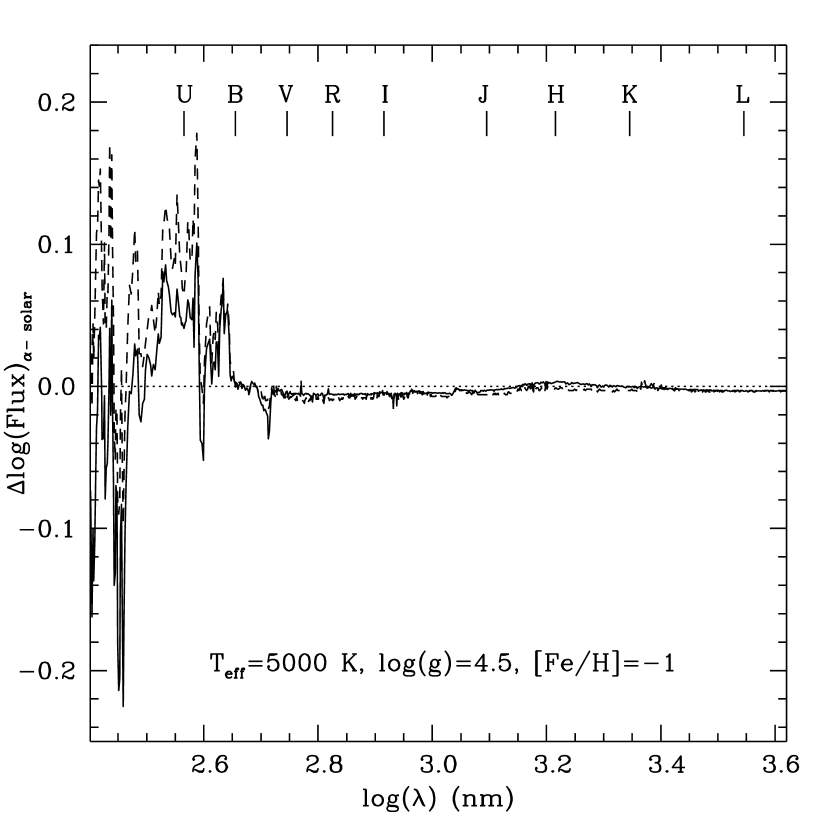
Figure 2: Difference of the logarithm of the flux (erg/$cm^{2}$/s/hz/ster) predicted for an $\alpha-$enhanced model $T_{eff}$=5000 K, log($g$)=4.5, [Fe/H]=$-$1.0 ([M/H]=$-$0.7), and a corresponding scaled-solar model with either the same [Fe/H] (solid line) or the same [M/H] (dashed line). Wavelengths are in nm; the effective wavelengths of various broadband filters are also marked.

When considering the case of scaled-solar transformations with the same [Fe/H] of the $\alpha-$enhanced mixture, the results are practically identical at [Fe/H] of the order of $-$2.0 and in general one obtains a better agreement with the appropriate $\alpha-$enhanced transformations; however, the discrepancies are non negligible when Z$\sim$0.001, increasing with both metal content and decreasing $T_{eff}$. At first it may appear surprising that $(B-V)$ and $(U-B)$ colors at the same [Fe/H] are bluer in the $\alpha-$enhanced case, when the total metal content is higher. Figure 2 shows the differences between the flux predicted for a typical $\alpha-$enhanced MS model with [Fe/H]=$-$1, and scaled-solar models with either the same [Fe/H] (solid line) or the same [M/H] (dashed line). The $\alpha-$enhanced model shows a larger flux in the $UB$ part of the spectrum with respect to the scaled-solar counterpart with the same [Fe/H], and a qualitative analysis of the figure shows clearly that the $\alpha-$enhanced $(U-B)$ and $(B-V)$ indices have to be bluer. On the other hand, colors built from passbands bluer than $U$ may provide different results. It is in fact evident from Fig. 2 that, e.g., around $\lambda$=280 nm (log($\lambda$)$\sim$2.45) the $\alpha-$enhanced flux is definitely lower than the scaled-solar counterparts.

In order to explain the differences highlighted by Fig. 2, one needs to assess the role played by the different $\alpha-$elements in modifying the stellar flux with respect to a scaled-solar mixture. It is clear that, for an exhaustive analysis, one should compute a set of model atmospheres for several gravities and effective temperatures, by changing the abundance of each individual $\alpha$ element at constant [Fe/H]. This notwithstanding – prompted by the referee – we have obtained relevant preliminary results by computing selected models for the same [Fe/H], gravity and $T_{eff}$ as in Fig. 2, enhancing once at a time the abundances of the most relevant $\alpha-$elements, i.e. O, Si, Mg and Ca.

As a general point, the different metal distributions of the $\alpha-$enhanced and scaled-solar models, computed for the same $T_{eff}$ and gravity, affect both the line opacity and the continuum opacity, redistributing the flux among the various wavelengths in such a way that the flux conservation $\int_{0}^{\infty}{F_{\nu}d\nu}=\sigma T_{eff}^{4}/\pi$ is met. For any abundance change the shape of the flux distribution is modified, due to a change of either the continuum level, or the line absorption or both. For instance, the $\alpha$ element that mostly affects the level of the continuum in our model is Mg, owing to the occurrence of a Mg I ionization edge at 2500$\AA$. By increasing the Mg abundance the continuum flux decreases shortward of the Mg I discontinuity and increases longward of it. Instead, the oxygen abundance affects the flux distribution in the region of the U and V bands through the numerous OH lines lying mostly shortward of the Balmer discontinuity.

Figure 3 shows differences $\Delta$(Flux) between the flux predicted for models with only the labeled $\alpha$ element enhanced (by 0.4 dex each), and the scaled solar case with the same [Fe/H]=$-$1.0, $T_{eff}=5000K$ and $\log(g)=4.5$. The $\Delta$(Flux) values between the complete $\alpha$-enhanced model and the scaled solar one with the same [Fe/H], $T_{eff}$ and $\log(g)$ is also displayed. We focused our analysis on the wavelength region where the largest $\Delta$(Flux) values contributing to the discrepancies in the $U$ and $B$ filters are found.

One can notice how $\Delta$(Flux) between the complete $\alpha$-enhanced model and the scaled solar one is essentially due to just O, Si, Mg and Ca. Calcium contributes mainly to the absorption at $\lambda\sim$390 nm, whereas O and Mg play a major role in the differences at $\lambda>350$ nm (apart from the Ca absorption mentioned before). In addition, Si and Mg are the most important contributors to the region shortward of $\sim$350 nm.

Table 1 displays the $(U-B)$ and $(B-V)$ colors predicted by the same model atmospheres whose flux difference are shown in Fig. 3; this allows us to assess quantitatively how much these individual $\alpha$ elements affect the broadband $UBV$ colors. Magnesium appears to be the main responsible for the $(B-V)$ and $(U-B)$ color differences between the scaled solar mixture and the full $\alpha-$enhanced one; in fact, by enhancing only Mg one recovers 88% and 76% of the differences in $(B-V)$ and $(U-B)$, respectively. Oxygen has a smaller but non negligible impact on the $(B-V)$ color whereas the $(U-B)$ color is affected appreciably also by silicon. Calcium and the other $\alpha$ elements have only a minor impact on these two colors at this $T_{eff}$ and gravity.

Prompted by our referee, to investigate the effects due to surface gravity changes along an isochrone, we have computed additional model atmospheres by enhancing the abundance of each individual $\alpha-$element, at the same [Fe/H] and effective temperature as above, but for $\log(g)=3.0$. We obtain results similar to the case with $\log(g)=4.5$ – as one could also expect by comparing the CT tables for scaled solar and full $\alpha$-enhanced mixtures at these two gravities – the main difference being that, whereas at $\log(g)=4.5$ the most important $\alpha-$element for the $UB$ flux distribution is Mg, in this case the contributions provided by Mg and Si are comparable.

Table 2 lists the differences between some relevant features of the three sets of isochrones displayed in Fig. 1. In particular, we wish to briefly discuss the $(B-V)$ color of the Main Sequence (MS) at M_V=6 ($(B-V)_{\rm M_{\sl V}=6}$), the absolute visual magnitude of the Turn Off (TO), the color difference $(\Delta(B-V))$ between the TO and the Red Giant Branch (RGB), the absolute I-Cousins magnitude of the RGB tip and the absolute visual magnitude of the ZAHB at the level of the instability strip. These quantities are usually employed in studies about distance and age determinations of old stellar populations. In the following we will refer to the use of scaled-solar transformations with the same [M/H] of the $\alpha-$enhanced mixture, which produce the larger differences.

The $(B-V)_{\rm M_{\sl V}=6}$ color (taken as representative magnitude of the unevolved MS in globular clusters) enters the MS fitting method for deriving cluster distances (e.g., Carretta et al. 2000, Percival et al. 2002). In fact, the color shifts applied to individual subdwarfs in order to ‘register’ their own metallicity to that of the considered cluster, are usually derived from theoretical isochrones, at least in the regime of globular cluster metallicities. The data listed in Table 2 show that the $(B-V)_{\rm M_{\sl V}=6}$ difference between the metallicities displayed in Fig. 1 does depend on the choice of the transformations, and are about 20% smaller when using the appropriate $\alpha-$enhanced transformations. This discrepancy may however have only a small impact on the derived distances as long as the subdwarfs employed in the MS-fitting have metallicities close to the cluster one, hence the color shifts applied are small.

The $(B-V)$ color extension between TO and RGB, $\Delta(B-V)$, is also clearly strongly affected. Following Rosenberg et al. (1999), here we have defined $\Delta(B-V)$ as the color difference between the TO and a point on the RGB 2.5 mag brighter than the TO. This quantity is a function of the cluster age, but it is generally used only in a differential way in order to determine relative cluster ages (e.g. Vandenberg, Bolte & Stetson 1990, Salaris & Weiss 1998, Rosenberg et al. 1999). The absolute values of $\Delta(B-V)$ change by $\sim$ 0.03-0.04 mag, depending on the metallicity; this would cause an age variation by $\sim$ 2-3 Gyr if $\Delta(B-V)$ is used to estimate absolute ages. When differences of $\Delta(B-V)$ at varying ages are used for relative age estimates, the impact of the CT transformation choice is however almost negligible.

As for the M_V values of TO and ZAHB at the RR Lyrae instability strip – whose difference is usually employed to estimate cluster ages – they are affected by the adopted CT relation at the level of $\approx$ 0.01 mag, which has a negligible impact on the age estimates. We have in addition verified that, at a fixed metallicity, the range of masses populating the RR Lyrae instability strip is basically unaffected by the choice of the transformations. Also the $I$ magnitude of the RGB Tip (a widely used distance indicator for old stellar populations, see e.g. Lee, Freedman & Madore 1993, Salaris & Cassisi 1998 and references therein) is unaffected by the choice of the transformations, the variation being of the order of $\sim$0.01 mag, which has a negligible impact on the distance determinations.

4 Treatment of surface boundary conditions

It is well known that in order to integrate the stellar structure equations, it is necessary to fix the value of the pressure and temperature at the stellar surface, usually close to the photosphere. There are basically two possibilities to determine this value. The first one is to integrate the atmospheric layers by using a $T(\tau)$ relationship, supplemented by the hydrostatic equilibrium condition and the equation of state; the second possibility is to obtain the required boundary conditions from precomputed non-gray model atmospheres.

The first procedure is universally used in stellar model computation; i.e., in our stellar evolution calculations employed above we have used the Krishna-Swamy (1966) solar $T(\tau)$ relationship. In Salaris, Cassisi & Weiss (2002) we have already shown that in case of scaled-solar models, the $T(\tau)$ integration and boundary conditions from model atmospheres (belonging to a previous ATLAS 9 release) provide RGB tracks that agree within about 50 K.

Here we repeat the test on scaled-solar models and for the first time we add a corresponding test for an $\alpha$-enhanced mixture, using the updated ATLAS 9 model grid discussed in the previous section. Figure 4 shows the evolutionary tracks of a 0.9$M_{\odot}$ star with a turn off age of $\sim$ 10.5 Gyr, from the beginning of the MS up to the RGB tip, in the log$L/L_{\odot}$-$T_{eff}$ plane. Four different tracks are displayed, corresponding to the pair Z=0.004, Y=0.251, for scaled solar and $\alpha$-enhanced metal distributions, computed using boundary conditions from both a $T(\tau)$ integration and non-gray model atmospheres with the appropriate metal mixture. The boundary conditions from the model atmospheres were taken at $\tau$=56. In both scaled-solar and $\alpha$-enhanced case the MS is completely insensitive to the choice of the boundary conditions. The RGB part is slightly affected, at the level of at most 40 K, the model atmosphere tracks being cooler. The effect of this temperature change on the predicted colors is the following: $\Delta(B-V)\approx+0.02$ mag, $\Delta(U-B)\approx+0.03$ mag, $\Delta(V-I)\approx+0.02$ mag.

Evolutionary timescales and interior properties of the models are also unaffected by the choice of the boundary conditions. Analogous results have been obtained at different Z. We also computed a model for $M=0.9M_{\odot}$, Z=0.004, by taking the model atmosphere boundary conditions at $\tau$=10, obtaining the same results as for the $\tau$=56 case.

We therefore conclude that scaled-solar and $\alpha$-enhanced isochrones can be safely computed - within the quoted uncertainty of about 40 K - integrating a solar $T(\tau)$ relationship for the boundary conditions, at least when the evolving mass is larger than $\sim 0.5-0.6M_{\odot}$ (which is the lower mass limit of our isochrones); lower masses may be more affected by the choice of the boundary conditions, as discussed, e.g., in Alexander et al. (1997), Chabrier & Baraffe (1997) and references therein. Moreover the results of all previously published comparisons between scaled-solar and $\alpha$-enhanced models in the log$L/L_{\odot}$-$T_{eff}$ plane (e.g., Salaris et al. 1993, Vandenberg et al. 2000) that were computed employing $T(\tau)$-based boundary conditions, are fully confirmed when employing the boundary conditions from the appropriate non-gray model atmospheres.

Our results suggest that employing a solar $T(\tau)$ relationship for the boundary conditions provides a fair approximation to the boundary conditions from non-gray model atmospheres, although in principle it is more appropriate and self-consistent to rely on model atmosphere results. This notwithstanding, one has to consider the fact that also model atmospheres are affected by intrinsic uncertainties, especially related to convection, and are usually based on a convection treatment different from the one adopted in stellar evolution computations (Montalban et al. 2001).

Figure 5 compares 12 Gyr old isochrones for a scaled solar mixture and for an $\alpha-$enhanced one with the same global metallicity, computed by using both boundary conditions and CT transformations from the appropriate model atmospheres. The equivalence between scaled-solar and $\alpha-$enhanced isochrones with the same [M/H] is still good at low metallicities, especially in the $VI$ plane, while in the $BV$ plane there are small differences due to the effect of the CT transformations. Larger differences are present at $Z\approx$0.004, especially significant in the $BV$ plane.

5 Summary

We have compared updated ATLAS 9 $UBVRIJHKL$ synthetic photometry for both $\alpha-$enhanced and scaled-solar metal distributions, in a large range of metallicities typical of the Galactic halo populations. This is the first complete analysis of the impact of an [$\alpha$/Fe]$>$0 metal distribution on broadband colors and bolometric corrections, for the full metallicity range of the Galactic halo population.

We found that it is impossible to mimic the appropriate $\alpha-$enhanced $(B-V)$ and $(U-B)$ color transformations with simple rescalings of the scaled-solar ones, over the entire [Fe/H] range of the Galactic halo. At [Fe/H]$\sim-$2.0 $\alpha-$enhanced transformations are well reproduced by scaled-solar ones with the same [Fe/H], however, this good agreement breaks down for [Fe/H] larger than about $-$1.6. In general, $(B-V)$ and $(U-B)$ $\alpha-$enhanced colors tend to be bluer than scaled-solar ones at either the same [Fe/H] or [M/H], and the differences increase with increasing metallicity and decreasing $T_{eff}$. These differences are mainly due to the enhancement of Mg with contributions from the enhancement of Si and O.

On the other hand $BC_{V}$ and more infrared colors predicted by $\alpha-$enhanced transformations are well reproduced by scaled-solar results. Key quantities like the TO and ZAHB $V$ magnitudes, as well as the RGB tip $I$ magnitude obtained from theoretical isochrones are basically unaffected by the use of the appropriate $\alpha-$enhanced transformations.

We have also tested for the first time the effect of boundary conditions obtained from appropriate $\alpha$-enhanced model atmospheres on the stellar evolutionary tracks in the log$L/L_{\odot}$-$T_{eff}$ plane. We find that, as in case of scaled solar models, the integration of a solar $T(\tau)$ relationship provides – at least for masses larger than 0.5 – 0.6 $M_{\odot}$ – $\alpha$-enhanced tracks very similar to the ones computed using boundary conditions from the appropriate model atmospheres.

Table 1: Colors predicted by model atmospheres computed for a scaled solar mixture, a fully $\alpha-$enhanced one, and by changing the abundance of each individual $\alpha$ element at constant [Fe/H] (see text for details).

Color	scaled solar	$\alpha-$enhanced	$Mg_{+0.4}$	$O_{+0.4}$	$Si_{+0.4}$	$Ca_{+0.4}$
$(B-V)$	0.841	0.793	0.799	0.813	0.839	0.850
$(U-B)$	0.322	0.231	0.253	0.314	0.284	0.324

Table 2: Selected properties of 12 Gyr old $\alpha-$enhanced isochrones with the labeled metallicities; the table displays differences (in mag) between the values obtained using the the appropriate $\alpha-$enhanced transformations, and scaled-solar ones with either the same [M/H] or the same [Fe/H] (see text for details).

CT transformations	$(B-V)_{\rm M_{\sl V}=6}$	MV(TO)	$\Delta(B-V)$	MI(TRGB)	MV(ZAHB)
Z=0.001
scaled-solar (same [M/H])	$-$0.027	0.014	$-$0.031	0.003	0.009
scaled-solar (same [Fe/H])	$-$0.006	0.030	$-$0.012	0.008	$-$0.001
Z=0.004
scaled-solar (same [M/H])	$-$0.052	0.008	$-$0.042	0.002	0.009
scaled-solar (same [Fe/H])	$-$0.028	$-$0.014	$-$0.027	$-$0.001	$-$0.002
Z=0.01
scaled-solar (same [M/H])	$-$0.072	$-$0.019	$-$0.044	0.001	0.012
scaled-solar (same [Fe/H])	$-$0.041	0.003	$-$0.028	0.023	$-$0.004

Figure 1: CMDs of 12 Gyr old $\alpha-$enhanced isochrones with the labeled metallicities. Three different sets of CT transformations have been employed. Solid lines represent $\alpha-$enhanced transformations with the appropriate metal mixture; long dashed lines denote scaled-solar transformations with the same [Fe/H] of the $\alpha-$enhanced ones, whereas short dashed lines display the case of scaled-solar transformations with the same [M/H] of the $\alpha-$enhanced ones. The inset shows an enlargement of the RGB section of the Z=0.01 isochrone, to enhance the difference between the location of the solid and long dashed lines. The horizontal dotted line marks the $M_{V}=6$ level (see text for details).

Figure 3: As in Fig. 2 but for 4 partial $\alpha$-enhanced mixtures where only the labeled elements are enhanced with respect to Fe ([$\alpha$/Fe]=0.4). All mixtures have [Fe/H]=$-$1.0; the solid line displays the difference between the complete $\alpha$-enhanced distribution and the solar one (it corresponds to the solid line in Fig. 2), while dashed lines show the differences between the various partial $\alpha$-enhanced mixtures and the solar one.

Figure 4: Comparison on the log$L/L_{\odot}$-$T_{eff}$ plane of 0.9$M_{\odot}$ stellar models with Z=0.004 (scaled-solar and $\alpha$-enhanced) computed using boundary conditions from model atmospheres (dashed lines) and from the integration of a $T(\tau)$ relationship (solid line).

Figure 5: CMDs of 12 Gyr old isochrones computed by adopting a scaled solar mixture (dashed lines) and an $\alpha-$enhanced one (solid lines) but the same global metallicity (the adopted metallicities are labeled in the panels). For each adopted heavy element mixture, the boundary conditions in the stellar evolutionary computations as well as the CT transformation have been consistently derived by an appropriate set of model atmospheres.

References

- (1) Alexander, D.R., Brocato, E., Cassisi, S., Castellani, V., Ciacio, F. & Degl’Innocenti, S. 1997, A&A, 317, 90
- (2) Azusienis, A., & Straižys, V. 1969, Soviet. Astron. AJ 13, 316
- (3) Anders, E. & Grevesse, N. 1989, Geochimica et Cosmochimica Acta, 53, 197
- (4) Barbuy, B. 1994, A&A, 430, 218
- (5) Barbuy, B., Perrin, M.-N., Katz, D., Coelho, P., Cayrel, R., Spite, M. & Van’t Veer-Menneret, C. 2003, A&A, 404, 661
- (6) Bessell, M.S. 1990, PASP 102, 1181
- (7) Bessell, M.S., & Brett, J.M. 1988, PASP 100, 1134
- (8) Buser, R. 1978, A&A 62, 411
- (9) Bessell, M.S., Castelli, F. & and Plez, B. 1998, A&A333, 231
- (10) Carretta, E., Gratton, R.G., Clementini, G. & Fusi Pecci, F. 2000, ApJ, 533, 215
- (11) Cassisi, S., Salaris, M. & Irwin, A.W. 2003, ApJ, 588, 862
- (12) Castelli, F. 1999, A&A346, 564
- (13) Castelli, F. & Kurucz, R.L. 2001, A&A372, 260
- (14) Castelli, F., & Kurucz, R.L. 2003, in Modeling of Stellar Atmospheres, IAU Symp. 210 (N.E. Piskunov et al., eds.), poster A20 on the enclosed CD-ROM (astro-ph/0405087)
- (15) Chabrier, G. & Baraffe,I. 1997, A&A, 327, 1039
- (16) Franchini, M., Morossi, C., di Marcantonio, P., Malagnini, M.L., Chavez, M. & Rodriguez-Merino, L. 2004, ApJ, 601, 485
- (17) Grevesse, N., & Sauval, A.J. 1998, Space Sci. Rev. 85, 161
- (18) Johnson, H.L. 1965, ApJ 141, 923
- (19) Kim, Y.-C., Demarque, P., Yi, S.K. & Alexander, D.R. 2002, ApJS, 143, 499
- (20) Krishna-Swamy, K.S. 1966, ApJ, 145, 174
- (21) Kurucz, R.L. 1993, ATLAS9 Stellar Atmosphere Programs and 2Km/s grid, CD-Rom n. 13
- (22) Lambert, D.L. 1989, in Cosmic Abundances of Matter, ed. C.J. Waddington (New York:AIP), 168
- (23) Lamla, E. 1982, in Landolt-Börstein, Neue Serie, (K. Schaifers, H.H. Voigt eds.), p.71
- (24) Lee, M.G., Freedman, W. & Madore, B.F. 1993, ApJ, 417, 553
- (25) McQuitty, R.J., Jaffe, T.R., Friel, E.D. & Dalle Ore, C.M. 1994, AJ, 107, 359
- (26) Montalban, J., Kupka, F., D’Antona, F. & Schmidt, W. 2001, A&A, 370, 982
- (27) Percival, S., Salaris, M., van Wyk, F. & Kilkenny, D. 2002, ApJ, 573, 174
- (28) Pietrinferni, A., Cassisi, S., Salaris, M. & Castelli, F. 2004, ApJ, in press (astro-ph/0405193)
- (29) Rosenberg, A., Saviane, I., Piotto, G. & Aparicio, A. 1999, AJ, 118, 2306
- (30) Salaris, M. & Cassisi, S. 1998, MNRAS, 298, 166
- (31) Salaris, M. & Weiss, A. 1998, A&A, 335, 943
- (32) Salaris, M. & Weiss, A. 2002, A&A, 388, 492
- (33) Salaris, M., Chieffi, A. & Straniero, O. 1993, ApJ, 414, 580
- (34) Salaris, M., Cassisi, S. & Weiss, A. 2002, PASP, 114, 375
- (35) Salaris, M., Riello, M., Cassisi, S. & Piotto, G. 2004, A&A, 420, 911
- (36) Salasnich, B., Girardi, L., Weiss, A. & Chiosi, C. 2000, A&A, 361, 1023
- (37) Thomas, D., Maraston, C. & Bender, R. 2003, MNRAS, 339, 897
- (38) Tripicco, M.J. & Bell, R.A. 1995, AJ, 110, 3035
- (39) Vandenberg, D.A., Bolte, M. & Stetson, P.B. 1990, AJ, 100, 445
- (40) Vandenberg, D.A., Swenson, F.J., Rogers, F. J., Iglesias, C.A. & Alexander, D.R. 2000, ApJ, 532, 430
- (41) Vazdekis, A., Cenarro, A.J., Gorgas, J., Cardiel, N. & Peletier, R.F. 2003, MNRAS, 340, 1317
- (42) Weiss, A., Peletier, R.F. & Matteucci, F. 1995, A&A, 296, 73