Parametric resonance as a model for QPO sources – I.
A general approach to multiple scales

Abstract

In the resonance model, high-frequency quasi-periodic oscillations (QPOs) are supposed to be a consequence of nonlinear resonance between modes of oscillations occurring within the innermost parts of an accretion disk. Several models with a prescribed mode–mode interaction were proposed in order to explain the characteristic properties of the resonance in QPO sources. In this paper, we examine nonlinear oscillations of a system having a quadratic nonlinearity and we show that this case is particularly relevant for QPOs. We present a very convenient way how to study internal resonances of a fully general system using the method of multiple scales. Finally, we concentrate to conservative systems and discuss their behavior near the $3:2$ resonance.

1 Introduction

In the resonance model (Abramowicz & Kluźniak, 2001; Kluźniak & Abramowicz, 2000; Kato, 2003), there is a natural and attractive possibility of explaining the observed rational ratios of high-frequency QPOs as a consequence of non-linear coupling between different modes of accretion disk oscillations. The idea has been pursued in several papers (recently, e.g. Abramowicz et al., 2003; Rebusco, 2004).

Specific models invoke particular physical mechanisms. Some models can be almost immediately comprehended as distinct realisations of the general approach discussed here – for example, various formulations of the orbiting spot model (Schnittman & Bertchinger, 2004) or the models, where QPOs are produced by the magnetically driven resonance in a diamagnetic accretion disk (Lai, 1999) – while other seem to be more distant from the view presented herein – e.g. the transition layer model (Titarchuk, 2002), an interesting idea of p-mode oscillations of a small accretion torus (Rezzola et al., 2003) or the model of blobs in an accretion disc (see e.g. Karas, 1999; Li & Narayan, 2004, and references cited therein). Also in this context, Kato, (2004) discussed the resonant interaction between waves propagating in a warped disk, including their rigorous mathematical description. Instead of pursuing a specific model, here we keep the discussion as general as possible, aiming to implement the formalism of multiple scales. Indeed, we show that there is unquestionable appeal in this approach which offers some additional insight into generic properties of resonant oscillations.

Some properties of an accretion disk oscillations can be discussed within the epicyclic approximation of a test particle on a circular orbit near equatorial plane. Suppose that angular momentum of the particle is fixed to a value $\ell$. The effective potential $U_{\ell}(r,\theta)$ has a minimum at radius $r_{0}$, corresponding to the location of the stable circular orbit. An observer moving along this orbit measures radial, vertical and azimuthal epicyclic oscillations of a particle nearby. Since the angular momentum of the particle is conserved, only two of them – radial and vertical – are independent. The epicyclic frequencies can be derived from the geodesic equations expanded to the linear order in deviations $\delta r=r-r_{0}$ and $\delta\theta=\theta-\pi/2$ from the circular orbit. We get two independent second-order differential equations describing two uncoupled oscillators with frequencies $\omega_{r}$ and $\omega_{\theta}$, which are given by the second derivatives of effective potential $U_{\ell}(r,\theta)$. In Newtonian theory, $\omega_{r}$ and $\omega_{\theta}$ are equal to the Keplerian orbital frequency $\Omega_{K}$. This is in tune with the fact that orbits of particles are planar and closed curves. The degeneracy between two epicyclic frequencies can be seen as a result of scale-freedom of the Newtonian gravitational potential (Abramowicz & Kluźniak, 2003). In Schwarzschild geometry this freedom is broken by introducing the gravitational radius $r_{g}=2GM/c^{2}$. The degeneracy between the vertical epicyclic and the orbital frequencies is related to spherical symmetry of the gravitational potential, which assures the existence of planar trajectories of particles. All three frequencies are different in the vicinity of a rotating Kerr black hole.

In addition, when nonlinear terms of geodesic equations are included, the two oscillations in $r$ and $\theta$ directions become coupled and variety of new phenomena connected to nonlinear nature of the equations appear. This rich phenomenology includes frequency shift of observed frequencies with respect to eigenfrequencies, presence of higher harmonics and subharmonics, drifts and parametric resonance. The first three are connected to nonlinear oscillations of each mode and the last one comes from the coupling between two modes.

The paper is organized in a following way: In the next section we will study one-degree-of-freedom system with a quadratic nonlinearity. We introduce the method of multiple scales (Nayfeh, 1973; Nayfeh & Mook, 1979) and, using this formalism, we derive key properties of nonlinear oscillations. In the third section we perform the multiple-scales expansion in the case of a fully general system of two coupled oscillators and find possible parametric resonances up to the fourth order. Then we concentrate on the $3:2$ parametric resonance of the conservative system.

2 Effects of nonlinearities

Let us consider the case of small but finite oscillations of a single-degree-of-freedom system with quadratic nonlinearity governed by equation

$$\ddot{x}+\omega^{2}x=\alpha\omega^{2}x^{2}.$$ (1)

The strength of the nonlinearity is parametrized by constant $\alpha$. When $\alpha=0$ one obtains governing equation of the corresponding linear system. We seek a perturbation expansion of the form

$$x(t,\epsilon)=\epsilon x_{1}(t)+\epsilon^{2}x_{2}(t)+\epsilon^{3}x_{3}(t)+{\cal O}(\epsilon^{4}),$$ (2)

The expansion parameter $\epsilon$ expresses the order of amplitude of oscillations. The main advantage of this approach is that, although the original equation is nonlinear, we solve linear equations in each step. For a practical purpose we require this expansion to be uniformly convergent for all times of interest. In that case the higher-order terms are small compared to lower-order terms and a sufficient approximation is reached concerning the finite number of terms. The expansion (2) can represent a periodic solution as well as an unbounded solution with exponential grow. The uniformity of the expansion means that the higher-order terms are not larger than the corresponding lower-order ones.

We substitute expansion (2) into governing equation (1) and, since $x_{k}$ is independent of $\epsilon$, we equate coefficients of corresponding powers of $\epsilon$ on both sides. This leads to the following system of equations

$$\ddot{x}_{1}+\omega^{2}x_{1} = 0,$$ (3)

$$\ddot{x}_{2}+\omega^{2}x_{2} = \alpha\omega^{2}x_{1}^{2},$$ (4)

$$\ddot{x}_{3}+\omega^{2}x_{3} = 2\alpha\omega^{2}x_{1}x_{2}.$$ (5)

The general solution of eq. (3) can be written in the form $x_{1}(t)=Ae^{i\omega t}+\mathrm{cc}$, where $\mathrm{cc}$ denotes complex conjugation. The complex constant $A$ contains information about the initial amplitude and phase of oscillations. Substituting it into eq. (4) we find linear equation for the first approximation $x_{2}(t)$

$$\ddot{x}_{2}+\omega^{2}x_{2}=\alpha\left(A^{2}e^{2i\omega t}+|A|^{2}\right)+\mathrm{cc}.$$ (6)

A general solution consists of the solution of the homogeneous equation and a particular solution,

$$x_{2}(t)=A_{2}e^{i\omega t}-\alpha\left(\frac{1}{3}A_{1}^{2}e^{2i\omega t}-|A_{1}|^{2}\right)+\mathrm{cc},$$ (7)

where $A_{1}$ denotes a constant $A$ of the solution of eq. (3). Therefore, the solution of governing equation up to the second order is given by

$$x(t)=\left(\epsilon A_{1}+\epsilon^{2}A_{2}\right)e^{i\omega t}-\alpha\left(\frac{1}{3}A_{1}^{2}e^{2i\omega t}-|A_{1}|^{2}\right)+\mathrm{cc}.$$ (8)

In fact, there are two possible ways how to satisfy general initial conditions $x(0)=\epsilon x_{0}$ and $\dot{x}(0)=\epsilon\dot{x}_{0}$ imposed on equation (1). The first one is to compare them with the general solution (8) and find constants $A_{1}$, $A_{2}$. This procedure should be repeated in each order of approximation which involves quite complicated algebra especially in higher orders. The second, equivalent and apparently much easier way is to include only particular solutions to the higher approximations and treat the constant $A$ as a function of $\epsilon$ with expansion $A=A_{1}+\epsilon A_{2}+\ldots$. Then, given initial conditions are satisfied by expanding the solution for $x_{1}$ via $\epsilon$ and choosing the coefficients $A_{n}$ appropriately.

According to this discussion we express the solution of eq. (6) as

$$x_{2}(t)=-\alpha\left(\frac{1}{3}A^{2}e^{2i\omega t}-|A|^{2}\right)+\mathrm{cc}.$$ (9)

Substituting $x_{1}$ and $x_{2}$ into (5) we obtain

$$\ddot{x}_{3}+\omega^{2}x_{3}=\frac{2\alpha^{2}\omega^{2}}{3}\left(5A|A|^{2}e^{i\omega t}-A^{3}e^{3i\omega t}\right)+\mathrm{cc}.$$ (10)

Since the right-hand side of this equation contains the term proportional to $e^{i\omega t}$, any solution must contain a secular term proportional to $te^{i\omega t}$, which becomes unbounded as $t\rightarrow\infty$. This fact has nothing to do with true physical behavior of the system for large times. The meaning is rather mathematical. Starting from time when $(\omega t)\sim 1/(\epsilon\alpha)$, the higher-order approximation $x_{3}$, which contains the secular term, does not provide only a small correction to $x_{1}$ and $x_{2}$, and the expansion (2) becomes singular. However, the presence of the secular term in the third order reflects very general feature of nonlinear oscillations – dependence of the observed frequency on the actual amplitude. For larger amplitudes the actual frequency of oscillations differs from the eigenfrequency $\omega$ and the higher-order terms in the expansion (2) – always oscillating with an integer multiples of $\omega$ – must quickly increase as time grows.

2.1 The method of multiple scales

Is it possible to find an expansion representing a solution of equation (1) which is uniformly valid even for larger time then $\sim\epsilon^{-1}$? Yes, if one considers more general form of the expansion than eq. (2). In the method of multiple scales more general dependence of coefficients $x_{i}$ on the time is reached by introducing several time scales $T_{\mu}$, instead of one physical time $t$. The time scales are introduced as

$$T_{\mu}\equiv\epsilon^{\mu}t, \mu=0,1,2\ldots$$ (11)

and they are treated as independent. It follows that instead of the single time derivative we have an expansion of partial derivatives with respect to the $T_{\mu}$

$$\frac{d}{dt} = D_{0}+\epsilon D_{1}+\epsilon^{2}D_{2}+\epsilon^{3}D_{3}+{\cal O}(\epsilon^{4}),$$ (12)

$$\frac{d^{2}}{dt^{2}} = D_{0}^{2}+2\epsilon D_{0}D_{1}+\epsilon^{2}(D_{1}^{2}+2D_{0}D_{2})+2\epsilon^{3}(D_{0}D_{3}+D_{1}D_{2})+{\cal O}(\epsilon^{4}),$$ (13)

where $D_{\mu}=\partial/\partial T_{\mu}$.

We assume that the solution can be represented by an expansion having the form

$$x(t,\epsilon)=\epsilon x_{1}(T_{\mu})+\epsilon^{2}x_{2}(T_{\mu})+\epsilon^{3}x_{3}(T_{\mu})+{\cal O}(\epsilon^{4}).$$ (14)

The number of time scales is always the same as the order at which the expansion is truncated. Here we carry out the expansion to the third order and thus first three scales $T_{0}$, $T_{1}$ and $T_{2}$ are sufficient.

Substituting eqs. (14) and (13) into the governing equation (1) and equating the coefficients of $\epsilon$, $\epsilon^{2}$ and $\epsilon^{3}$ to zero we obtain

$$(D_{0}^{2}+\omega^{2})x_{1} = 0,$$ (15)

$$(D_{0}^{2}+\omega^{2})x_{2} = -2D_{0}D_{1}x_{1}+\alpha\omega^{2}x_{1},$$ (16)

$$(D_{0}^{2}+\omega^{2})x_{3} = -2D_{0}D_{1}x_{2}-D_{1}^{2}x_{1}-2D_{0}D_{2}x_{1}+\alpha\omega^{2}x_{1}x_{2}.$$ (17)

Note that although these equations are more complicated than (3)–(5), they are still linear and can be solved successively. The solution of the equation (15) is the same as the solution of the corresponding linear system, the only difference is that constant $A$ now generally depends on other scales

$$x_{1}=A(T_{1},T_{2})e^{i\omega T_{0}}+\mathrm{cc}.$$ (18)

Substituting $x_{1}$ into the equation (16) we obtain

$$(D_{0}^{2}+\omega^{2})x_{2}=-2i\omega(D_{1}A)e^{i\omega T_{0}}+\alpha\omega^{2}\left(A^{2}e^{2i\omega T_{0}}+|A|^{2}\right)+\mathrm{cc}.$$ (19)

The first term on the right-hand side implies the presence of a secular term in the second-order approximation which causes non-uniformity of the expansion (14). However, in case of the method of multiple scales these terms can be eliminated by imposing additional conditions on the function $A(T_{\mu})$. These conditions are sometimes called conditions of solvability or conditions of consistency. In fact, the reason why the same number of scales as the order of approximation is needed is that one secular term gets eliminated in each order, and therefore the function $A(T_{\mu})$ is specified by the same number of solvability conditions as the number of its variables.

The secular term is eliminated if we require $D_{1}A=0$. In further discussion we assume that $A$ is a function of $T_{2}$ only. A particular solution of equation (19) is

$$x_{2}(t)=-\alpha\left(\frac{1}{3}A^{2}(T_{2})e^{2i\omega T_{0}}-|A(T_{2})|^{2}\right)+\mathrm{cc}.$$ (20)

Using the condition $D_{1}A=0$ the equation (17) takes much simpler form

$$(D_{0}^{2}+\omega^{2})x_{3}=-\left(2i\omega D_{2}A+\frac{10\alpha^{2}\omega^{2}}{3}A|A|^{2}\right)e^{i\omega T_{0}}-\frac{2\alpha^{2}\omega^{2}}{3}A^{3}e^{3i\omega T_{0}}+\mathrm{cc}.$$ (21)

The secular term is eliminated equating the terms in the bracket to zero

$$2i\omega D_{2}A+\frac{10\alpha^{2}\omega^{2}}{3}A|A|^{2}=0.$$ (22)

This additional condition fully determines (excepting initial conditions) time behavior of function $A(T_{2})$. Let us write it in the polar form $A=\frac{1}{2}\tilde{a}e^{i\phi}$ and then separate real and imaginary parts. We obtain

$$D_{2}\tilde{a}=0 \mathrm{and} D_{2}\phi=-\frac{5\alpha^{2}}{12}\omega\tilde{a}^{2}.$$ (23)

The solutions of these equations are

$$\tilde{a}=\tilde{a}_{0} \mathrm{and} \phi=-\frac{5}{12}\alpha^{2}\tilde{a}_{0}^{2}\omega T_{2}+\phi_{0},$$ (24)

where $\tilde{a}_{0}$ and $\phi_{0}$ are constants which are determined from the initial conditions.

It follows from eq. (18) that $A(T_{2})$ slowly modulates the amplitude and the phase of oscillations. Since $\tilde{a}$ is constant, the amplitude is constant all the time. Since $\phi$ depends on $T_{2}=\epsilon^{2}t$ linearly, also the observed frequency of the oscillations is constant, but not equal to the eigenfrequency $\omega$.

Substituting eqs. (24) and (20) into (14), we obtain solution of eq. (1) up to the second order

$$x(t)=a_{0}\cos(\omega^{\star}t+\phi_{0})-\frac{\alpha}{6}a_{0}^{2}\cos[2(\omega^{\star}t+\phi_{0})]+\frac{\alpha}{2}a_{0}^{2}+{\cal O}(a_{0}^{3}),$$ (25)

where $a_{0}=\epsilon\tilde{a}_{0}\ll 1$ and $\omega^{\star}$ is the observed frequency of oscillation given by

$$\omega^{\star}=\omega\left(1-\frac{5\alpha^{2}}{12}a_{0}^{2}\right).$$ (26)

2.2 Essential properties of nonlinear oscillations

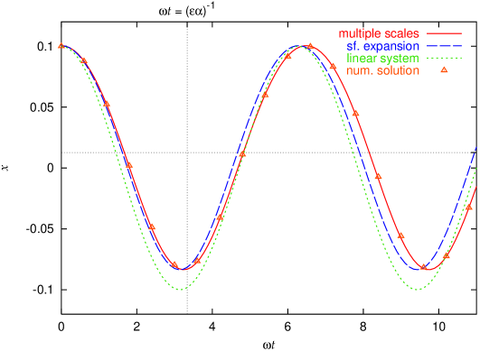
Figure 1: Oscillations of the system with quadratic nonlinearity governed by the equation (1). We compare results of the multiple scales method (solid curve), a simple straightforward expansion method (dashed curve) and the direct numerical integration of the governing equation (points). The initial condition is $x(0)=0.1$, $\dot{x}(0)=0$ and the strength of nonlinearity is $\alpha=3$. The horizontal dotted line shows the shifted ‘equilibrium position’ and the vertical one denotes the value $(\omega t)=(\epsilon\alpha)^{-1}$ at which the straightforward expansion becomes nonuniform. The solution corresponding to the linear system is also shown (dotted curve).

We close this section summarizing main properties of nonlinear oscillations. The equation (25) is very helpful for this purpose.

The leading term of the expansion (25) describes oscillations with frequency close to eigenfrequency of the system. Both the amplitude and the frequency are constant in time, but they are not independent (as in case of the linear approximation). The frequency correction given by (26) is proportional to the square of the amplitude. This fact is sometimes called the amplitude-frequency interaction and – as was mentioned above – it causes the non-uniformity of the expansion (2) (see the figure 1).

The second term oscillates with twice as large frequency and provides the second-order correction to the leading term. The presence of higher harmonics is another particular feature of nonlinear oscillations and the fact that it has been reported in several sources of QPOs, points to nonlinear nature of this phenomena.

The third term describes constant shift from the equilibrium position and is related to the asymmetry of the potential energy about the point $x=0$. In the linear analysis, this effect is not present because the potential energy depends on $x^{2}$, and therefore is symmetric with respect to the point $x=0$. Hence, the drift is the third characteristic feature of nonlinear oscillations.

3 Parametric resonances in conservative systems

Let us study nonlinear oscillations of the system having two degrees of freedom, i.e., the coordinate perturbations $\delta r$ and $\delta\theta$. The oscillations are described by two coupled differential equations of the very general form

$$\ddot{\delta r}+\omega_{r}^{2}\;\delta r = \omega_{r}^{2}\;f_{r}(\delta r,\delta\theta,\dot{\delta r},\dot{\delta\theta}),$$ (27)

$$\ddot{\delta\theta}+\omega_{\theta}^{2}\;\delta\theta = \omega_{\theta}^{2}\;f_{\theta}(\delta r,\delta\theta,\dot{\delta r},\dot{\delta\theta}).$$ (28)

Suppose that the functions $f_{r}$ and $f_{\theta}$ are nonlinear, i.e., their Taylor expansions start in the second order. Another assumption is that these functions are invariant under reflection of time (i.e., the Taylor expansion does not contain odd powers of time derivatives of $\delta r$ and $\delta\theta$). As we see later, this assumption is related to the conservation of energy in the system. Many authors studied such systems with a particular form of functions $f$ and $g$ (Nayfeh & Mook, 1979), however, in this paper we keep discussion fully general.

We seek the solutions of the governing equations in the form of the multiple-scales expansions

$$\delta r(t,\epsilon)=\sum_{n=1}^{4}\epsilon^{n}r_{n}(T_{\mu}), \delta\theta(t,\epsilon)=\sum_{n=1}^{4}\epsilon^{n}\theta_{n}(T_{\mu}),$$ (29)

where $T_{\mu}=\epsilon^{\mu}t$ are independent time scales, $\mu=0,1,2,3$ (we finish the discussion in the fourth order, however, it is possible to proceed to higher orders in suggested way). We expand the time derivatives according to eqs. (12) and (13) and equate terms of the same order in $\epsilon$ on both sides of the governing equations.

In the first order we obtain equations corresponding to the linear approximation

$$(D_{0}^{2}+\omega_{r}^{2})r_{1}=0, (D_{0}^{2}+\omega_{\theta}^{2})\theta_{1}=0.$$ (30)

with the solutions

$$x_{1}=\widehat{A}_{r}+\widehat{A}_{-r}, \theta_{1}=\widehat{A}_{\theta}+\widehat{A}_{-\theta},$$ (31)

where we denoted $\widehat{A}_{x}=A_{x}e^{i\omega_{x}T_{0}}$, $\widehat{A}_{-x}=A_{x}^{\ast}e^{-i\omega_{x}T_{0}}$, and $x=r$, $\theta$, respectively (since many considerations are independent of the mode of oscillations, we keep this notation through the whole section). The complex functions $\widehat{A}_{x}$ generally depend on the time-scales $T_{1}$, $T_{2}$, $T_{3}$.

Having solved the linear approximation, we can proceed to higher orders. The terms proportional to $\epsilon^{2}$ in the expanded left-hand side of the governing equation (27) resp. (28) are

$$\left[\ddot{\delta x}+\omega_{x}^{2}x\right]_{2}=(D_{0}^{2}+\omega_{x}^{2})x_{2}+2i\omega_{x}D_{1}\widehat{A}_{x}-2i\omega_{x}D_{1}\widehat{A}_{-x},$$ (32)

On the right-hand side there are second-order terms of the Taylor expansion of the nonlinearity $f(\delta r,\delta\theta,\dot{\delta r},\dot{\delta\theta})$, with $r_{1}$, $\theta_{1}$, $D_{0}r_{1}$ and $D_{0}\theta_{1}$ in the place of $\delta r$, $\delta\theta$, $\dot{\delta r}$ and $\dot{\delta\theta}$, respectively. Since the derivative with respect to $T_{0}$ only adds the coefficient $i\omega_{x}$, the second-order terms on the right-hand sides can be expressed as linear combinations of quadratic terms constructed from $\widehat{A}_{\pm r}$ and $\widehat{A}_{\pm\theta}$

$$\left[f_{x}(\delta r,\delta\theta,\dot{\delta r},\dot{\delta\theta})\right]_{2}=\omega_{x}^{2}\sum_{|\alpha|=2}C_{\alpha}^{(2,x)}\widehat{A}_{r}^{\alpha_{1}}\widehat{A}_{\theta}^{\alpha_{2}}\widehat{A}_{-r}^{\alpha_{3}}\widehat{A}_{-\theta}^{\alpha_{4}},$$ (33)

where $\alpha=(\alpha_{1},\ldots,\alpha_{4})$ and $|\alpha|=\alpha_{1}+\ldots+\alpha_{4}$. The constants $C_{\alpha}^{(2,x)}$ are combinations of $\omega_{x}$ and the coefficients in the Taylor expansion of functions $f$ and $g$, respectively. The coefficients coming from the terms containing time derivatives are generally complex, since each time derivative produces one “$i$”. However, if we suppose that the Taylor expansion does not contain odd powers of time derivatives, all of the constants $C_{\alpha}^{(2,x)}$ must be real. Equating right-hand sides of equations (32) and (33) we have

$$(D_{0}^{2}+\omega_{x}^{2})x_{2}=-2i\omega_{x}D_{1}\widehat{A}_{x}+2i\omega_{x}D_{1}\widehat{A}_{-x}+\omega_{x}^{2}\sum_{|\alpha|=2}C_{\alpha}^{(2,x)}\widehat{A}_{r}^{\alpha_{1}}\widehat{A}_{\theta}^{\alpha_{2}}\widehat{A}_{-r}^{\alpha_{3}}\widehat{A}_{-\theta}^{\alpha_{4}}.$$ (34)

$\omega_{\theta}:\omega_{r}$	Secular terms	Solvability condition
Outside	$D_{1}\widehat{A}_{r}$	$D_{1}\widehat{A}_{r}=0$
resonance	$D_{1}\widehat{A}_{\theta}$	$D_{1}\widehat{A}_{\theta}=0$
$1:2$	$\widehat{A}_{-r}\widehat{A}_{\theta}$	$-2iD_{1}\widehat{A}_{r}+\omega_{r}K\widehat{A}_{-r}\widehat{A}_{\theta}=0$
	$\widehat{A}_{r}^{2}$	$-2iD_{1}\widehat{A}_{\theta}+\omega_{\theta}L\widehat{A}_{r}^{2}=0$
$2:1$	$\widehat{A}_{\theta}^{2}$	$-2iD_{1}\widehat{A}_{r}+\omega_{r}K\widehat{A}_{\theta}^{2}=0$
	$\widehat{A}_{r}\widehat{A}_{-\theta}$	$-2iD_{1}\widehat{A}_{\theta}+L\widehat{A}_{r}A_{-\theta}=0$

Table 1: Possible resonances and appropriate solvability conditions in the second order of approximation. We substitute constants $C^{(n,x)}_{\alpha}$ by $K$ and $L$ for simplicity. The first record is related to the case when the system is far from any listed resonance. In this case only strictly secular terms are present. The first resp. second row in the record of each resonance is related to the equation for the radial resp. vertical oscillations. In that case, we list only nearly secular terms in the 2nd column, however strictly secular terms are included in the solvability conditions.

The right-hand side of equation (34) contains one secular term independently of the eigenfrequencies $\omega_{r}$ and $\omega_{\theta}$. However, in some particular cases, additional secular terms appear. For example, when $\omega_{r}\approx 2\omega_{\theta}$ the terms proportional to $\widehat{A}^{2}_{\theta}$ in the radial equation ($x\rightarrow r$) and $\widehat{A}_{r}\widehat{A}_{-\theta}$ in the meridional equation ($x\rightarrow\theta$) become nearly secular and they should be included in the solvability conditions. The analogical situation happens when $\omega_{r}\approx\omega_{\theta}/2$. These cases show qualitatively different behavior, and we speak about parametric or internal resonance. Possible resonances in the second order of approximation and appropriate solvability conditions are listed in the table 1. At this moment, let us assume that the system is far from the resonance and require

$$D_{1}A_{x}=0.$$ (35)

In this case the frequencies and the amplitudes are constant and the behavior of the system is almost the same as in the linear approximation. The only difference is the presence of the higher harmonics oscillating with the frequencies $2\omega_{r}$, $2\omega_{\theta}$ and $|\omega_{r}\pm\omega_{\theta}|$. They are given by a particular solution of equation (34) after elimination of secular term and can be expressed as a linear combination

$$x_{2}=\sum_{|\alpha|=2}Q_{\alpha}^{(2,x)}\widehat{A}_{r}^{\alpha_{1}}\widehat{A}_{\theta}^{\alpha_{2}}\widehat{A}_{-r}^{\alpha_{3}}\widehat{A}_{-\theta}^{\alpha_{4}}.$$ (36)

Under the assumption of invariance under the time reflection, constants $Q_{\alpha}^{(2,x)}$ are real and their relation to $C_{\alpha}^{(2,x)}$ becomes obvious, by substituting $x_{2}$ into equation (34).

When we proceed to the higher order, the discussion is analogical in many respects. The terms proportional to $\epsilon^{3}$, which appear on the left-hand side of the governing equations, are given by

$$\left[\ddot{\delta x}+\omega_{x}^{2}x\right]_{3}=(D_{0}^{2}+\omega_{x}^{2})x_{3}+2i\omega_{x}D_{2}\widehat{A}_{x}-2i\omega_{x}D_{2}\widehat{A}_{-x}.$$ (37)

The terms containing $D_{1}x_{1}$ and $D_{1}x_{2}$ vanish in consequence of the solvability condition (35). The right-hand side contains cubic terms of the Taylor expansion combined using first-order approximations $r_{1}$, $\theta_{1}$ and quadratic terms combined using one first-order – $r_{1}$ or $\theta_{1}$ – and one second-order quantity – $r_{2}$ or $\theta_{2}$. Since the second-order terms must be linear combinations of $\widehat{A}_{\pm r}$ and $\widehat{A}_{\pm\theta}$, the governing equations take the form

$$(D_{0}^{2}+\omega_{x}^{2})x_{3}=-2i\omega_{x}D_{2}\widehat{A}_{x}+2i\omega_{x}D_{2}\widehat{A}_{-x}+\omega_{x}^{2}\sum_{|\alpha|=3}C_{\alpha}^{(3,x)}\widehat{A}_{r}^{\alpha_{1}}\widehat{A}_{\theta}^{\alpha_{2}}\widehat{A}_{-r}^{\alpha_{3}}\widehat{A}_{-\theta}^{\alpha_{4}},$$ (38)

where all constants $C_{\alpha}^{(3,x)}$ are real.

$\omega_{\theta}:\omega_{r}$	Secular terms	Solvability condition
Outside	$D_{2}\widehat{A}_{r}$, $|A_{r}|^{2}\widehat{A}_{r}$, $|A_{\theta}^{2}|\widehat{A}_{r}$	$2iD_{2}\widehat{A}_{r}-\omega_{r}\left[\kappa_{r}|A_{r}|^{2}+\kappa_{\theta}|A_{\theta}|^{2}\right]\widehat{A}_{r}=0$
resonance	$D_{2}\widehat{A}_{\theta}$, $|A_{r}|^{2}\widehat{A}_{\theta}$, $|A_{\theta}^{2}|\widehat{A}_{\theta}$	$2iD_{2}\widehat{A}_{\theta}-\omega_{\theta}\left[\lambda_{r}|A_{r}|^{2}+\lambda_{\theta}|A_{\theta}|^{2}\right]\widehat{A}_{\theta}=0$
$1:3$	$\widehat{A}_{\theta}^{3}$	$2iD_{2}\widehat{A}_{r}-\omega_{r}\left[\kappa_{r}|A_{r}|^{2}+\kappa_{\theta}|A_{\theta}|^{2}\right]\widehat{A}_{r}+\omega_{r}K\widehat{A}_{\theta}^{3}=0$
	$\widehat{A}_{r}\widehat{A}_{-\theta}^{2}$	$2iD_{2}\widehat{A}_{\theta}-\omega_{\theta}\left[\lambda_{r}|A_{r}|^{2}+\lambda_{\theta}|A_{\theta}|^{2}\right]\widehat{A}_{\theta}+\omega_{\theta}L\widehat{A}_{r}\widehat{A}_{-\theta}^{2}=0$
$1:1$	$|A_{r}|^{2}\widehat{A}_{\theta}$, $|A_{\theta}|^{2}\widehat{A}_{\theta}$,	$2iD_{2}\widehat{A}_{r}-\omega_{r}\left[\kappa_{r}|A_{r}|^{2}+\kappa_{\theta}|A_{\theta}|^{2}\right]\widehat{A}_{r}+\omega_{r}\times\qquad$
	$\widehat{A}_{r}^{2}\widehat{A}_{-\theta}$, $\widehat{A}_{-r}\widehat{A}_{\theta}^{2}$	$(K_{1}|A_{r}|^{2}\widehat{A}_{\theta}+K_{2}|A_{\theta}|^{2}\widehat{A}_{\theta}+K_{3}\widehat{A}_{r}^{2}\widehat{A}_{-\theta}+K_{4}\widehat{A}_{-r}\widehat{A}_{\theta}^{2})=0$
	$|A_{r}|^{2}\widehat{A}_{r}$, $|A_{\theta}|^{2}\widehat{A}_{\theta}$,	$2iD_{2}\widehat{A}_{\theta}-\omega_{\theta}\left[\lambda_{r}|A_{r}|^{2}+\lambda_{\theta}|A_{\theta}|^{2}\right]\widehat{A}_{\theta}+\omega_{\theta}\times\qquad$
	$\widehat{A}_{-r}\widehat{A}_{\theta}^{2}$, $\widehat{A}_{r}^{2}\widehat{A}_{-\theta}$	$(L_{1}|A_{r}|^{2}\widehat{A}_{r}+L_{2}|A_{\theta}|^{2}\widehat{A}_{\theta}+L_{3}\widehat{A}_{-r}\widehat{A}_{\theta}^{2}+L_{4}\widehat{A}_{r}^{2}\widehat{A}_{-\theta})=0$
$3:1$	$\widehat{A}_{-r}^{2}\widehat{A}_{\theta}$	$2iD_{2}\widehat{A}_{r}-\omega_{r}\left[\kappa_{r}|A_{r}|^{2}+\kappa_{\theta}|A_{\theta}|^{2}\right]\widehat{A}_{r}+\omega_{r}K\widehat{A}_{-r}^{2}\widehat{A}_{\theta}=0$
	$\widehat{A}_{r}^{3}$	$2iD_{2}\widehat{A}_{\theta}-\omega_{\theta}\left[\lambda_{r}|A_{r}|^{2}+\lambda_{\theta}|A_{\theta}|^{2}\right]\widehat{A}_{\theta}+\omega_{\theta}L\widehat{A}_{r}^{3}=0$

Table 2: Possible resonances in the third order of approximation.

The secular terms together with possible resonances are summarized in the table 2. Far from any resonance, we eliminate the terms which are secular independently of $\omega_{r}$ and $\omega_{\theta}$. Multiplying by $e^{-i\omega_{x}t}$, the solvability conditions take the form

$$D_{2}A_{r}=-\frac{i\omega_{r}}{2}\left[\kappa_{r}|A_{r}|^{2}+\kappa_{\theta}|A_{\theta}|^{2}\right]A_{r},$$ (39)

$$D_{2}A_{\theta}=-\frac{i\omega_{\theta}}{2}\left[\lambda_{r}|A_{r}|^{2}+\lambda_{\theta}|A_{\theta}|^{2}\right]A_{\theta},$$ (40)

where we denoted $\kappa_{r}=C^{(3,r)}_{2010}$, $\kappa_{\theta}=C^{(3,r)}_{1101}$ , $\lambda_{r}=C^{(3,\theta)}_{1110}$ and $\lambda_{\theta}=C^{(3,\theta)}_{0201}$ because of simpler notation. A particular solution of equation (38) is given by linear combination of cubic terms constructed from $\widehat{A}_{\pm r}$ and $\widehat{A}_{\pm\theta}$

$$x_{3}=\sum_{|\alpha|=3}Q_{\alpha}^{(3,x)}\widehat{A}_{r}^{\alpha_{1}}\widehat{A}_{\theta}^{\alpha_{2}}\widehat{A}_{-r}^{\alpha_{3}}\widehat{A}_{-\theta}^{\alpha_{4}},$$ (41)

where all coefficients $Q_{\alpha}^{(3,x)}$ are real.

The terms proportional to $\epsilon^{4}$ in the expanded left-hand side of the equations (27) and (28) are

$$\left[\ddot{\delta x}+\omega_{x}^{2}x\right]_{4}=(D_{0}^{2}+\omega_{x}^{2})x_{3}+2D_{3}D_{0}x_{1}+2D_{0}D_{2}x_{2}.$$ (42)

The operator $D_{0}D_{2}$ acts on $x_{2}$ given by (36). The result is found using the solvability conditions (39), (40) and can be written in the form

$$2D_{0}D_{2}x_{2}=\omega_{x}^{2}\sum_{|\alpha|=4}J_{\alpha}^{(x)}\widehat{A}_{r}^{\alpha_{1}}\widehat{A}_{\theta}^{\alpha_{2}}\widehat{A}_{-r}^{\alpha_{3}}\widehat{A}_{-\theta}^{\alpha_{4}}.$$ (43)

where constants $J^{(x)}_{\alpha}$ are real because both $D_{0}$ and $D_{2}$ produce one “$i$”. The right-hand side is expanded similarly. We obtain

$$(D_{0}^{2}+\omega_{x}^{2})x_{4}=-2i\omega_{x}D_{3}\widehat{A}_{x}+2i\omega_{x}D_{3}\widehat{A}_{-x}+\omega_{x}^{2}\sum_{|\alpha|=4}C_{\alpha}^{(4,x)}\widehat{A}_{r}^{\alpha_{1}}\widehat{A}_{\theta}^{\alpha_{2}}\widehat{A}_{-r}^{\alpha_{3}}\widehat{A}_{-\theta}^{\alpha_{4}},$$ (44)

with real $C_{\alpha}^{(4,x)}$. On the right-hand side there is only one secular term $-2i\omega_{x}D_{3}\widehat{A}_{x}$ independently of $\omega_{r}$ and $\omega_{\theta}$, the sum contains only terms which becomes secular near a resonance. These terms and solvability conditions are listed in the table 3.

$\omega_{\theta}:\omega_{r}$	Secular terms	Solvability condition
Outside	$D_{3}\widehat{A}_{r}$	$D_{3}\widehat{A}_{r}=0$
resonance	$D_{3}\widehat{A}_{\theta}$	$D_{3}\widehat{A}_{\theta}=0$
$1:4$	$\widehat{A}_{\theta}^{4}$	$2iD_{3}\widehat{A}_{r}-\omega_{r}K\widehat{A}_{\theta}^{4}=0$
	$\widehat{A}_{r}\widehat{A}_{\theta}^{3}$	$2iD_{3}\widehat{A}_{\theta}-\omega_{\theta}L\widehat{A}_{r}\widehat{A}_{\theta}^{3}=0$
$2:3$	$\widehat{A}_{r}\widehat{A}_{-\theta}^{3}$	$2iD_{3}\widehat{A}_{r}-\omega_{r}K\widehat{A}_{r}\widehat{A}_{-\theta}^{3}=0$
	$\widehat{A}_{r}^{2}\widehat{A}_{-\theta}^{2}$	$2iD_{3}\widehat{A}_{\theta}-\omega_{\theta}L\widehat{A}_{r}^{2}\widehat{A}_{-\theta}^{2}=0$
$3:2$	$\widehat{A}_{-r}^{2}\widehat{A}_{\theta}^{2}$	$2iD_{3}\widehat{A}_{r}-\omega_{r}K\widehat{A}_{-r}^{2}\widehat{A}_{\theta}^{2}=0$
	$\widehat{A}_{r}^{3}\widehat{A}_{-\theta}$	$2iD_{3}\widehat{A}_{\theta}-\omega_{\theta}L\widehat{A}_{r}^{3}\widehat{A}_{-\theta}=0$
$4:1$	$\widehat{A}_{r}^{3}\widehat{A}_{\theta}$	$2iD_{3}\widehat{A}_{r}-\omega_{r}K\widehat{A}_{r}^{3}\widehat{A}_{\theta}=0$
	$A_{r}^{4}$	$2iD_{3}\widehat{A}_{\theta}-\omega_{\theta}L\widehat{A}_{r}^{4}=0$

Table 3: Possible resonances in the fourth order of approximation.

One general feature of an internal resonance $k:l$ is that $k\omega_{r}$ and $l\omega_{\theta}$ need not to be infinitesimally close. Consider, for example, resonance $1:2$. The resonance occurs when $\omega_{\theta}\approx 2\omega_{r}$. Suppose that the system departs from this exact ratio by small (first-order) deviation $\omega_{\theta}=2\omega_{r}+\epsilon\sigma$, where $\sigma$ is called detuning parameter. Then the terms $\widehat{A}_{-r}\widehat{A}_{\theta}$ and $\widehat{A}_{r}^{2}$ in the equations (34) remain still secular in $T_{0}$ since

$$\widehat{A}_{-r}\widehat{A}_{\theta}=A_{r}^{\ast}A_{\theta}e^{i(\omega_{\theta}-\omega_{r})T_{0}}=A_{r}^{\ast}A_{\theta}e^{i(\omega_{r}+\epsilon\sigma)T_{0}}=A_{r}^{\ast}A_{\theta}e^{i\sigma T_{1}}e^{i\omega_{r}T_{0}}$$ (45)

and analogically for $\widehat{A}_{r}^{2}$.

4 The 3:2 parametric resonance

Let us study oscillations of the conservative system which eigenfrequencies $\omega_{r}$ and $\omega_{\theta}$ are close to $3:2$ ratio. The time behavior of the observed frequencies $\omega^{\star}_{r}$ and $\omega^{\star}_{\theta}$ and amplitudes $a_{r}$ and $a_{\theta}$ of the oscillations is given by the solvability conditions (35), (39) and (40). In the fourth order we eliminate terms which become nearly secular. For this purpose let us introduce detuning parameters $\sigma_{2}$ and $\sigma_{3}$ according to

$$3\omega_{r}=2\omega_{\theta}+\epsilon^{2}\sigma_{2}+\epsilon^{3}\sigma_{3},$$ (46)

where the term $\epsilon\sigma_{1}$ is missing, because the complex amplitude $A$ depends only on time-scales $T_{2}$ and $T_{3}$. The secular terms in eq. (44) are eliminated if (see table 3)

$$2iD_{3}A_{r}-\omega_{r}\alpha(A_{r}^{2})^{\ast}A_{\theta}^{2}e^{-i(\sigma_{2}T_{2}+\sigma_{3}T_{3})} = 0,$$ (47)

$$2iD_{3}A_{\theta}-\omega_{\theta}\beta A_{r}^{3}A_{\theta}^{\ast}e^{i(\sigma_{2}T_{2}+\sigma_{3}T_{3})} = 0,$$ (48)

where $\alpha$ and $\beta$ are real constants depending on properties of the system. Since $A_{r}$ and $A_{\theta}$ are complex, the conditions (47) and (48) together with (35) and (39) represents 8 real equations. This can be seen by substituting the polar forms $A_{r}=\frac{1}{2}\tilde{a}_{r}e^{i\phi_{r}}$ and $A_{\theta}=\frac{1}{2}\tilde{a}_{\theta}e^{i\phi_{\theta}}$, and by separating real and imaginary parts. We obtain

$$D_{2}\tilde{a}_{r} = 0,$$ (49)

$$D_{2}\tilde{a}_{\theta} = 0,$$ (50)

$$D_{2}\phi_{r} = -\frac{\omega_{r}}{8}\left[\kappa_{r}\tilde{a}_{r}^{2}+\kappa_{\theta}\tilde{a}_{\theta}^{2}\right],$$ (51)

$$D_{2}\phi_{\theta} = -\frac{\omega_{\theta}}{8}\left[\lambda_{r}\tilde{a}_{r}^{2}+\lambda_{\theta}\tilde{a}_{\theta}^{2}\right],$$ (52)

$$D_{3}\tilde{a}_{r} = \frac{\alpha\omega_{r}}{16}\tilde{a}_{r}^{2}\tilde{a}_{\theta}^{2}\sin(-3\phi_{r}+2\phi_{\theta}-\sigma_{2}T_{2}-\sigma_{3}T_{3}),$$ (53)

$$D_{3}\tilde{a}_{\theta} = \frac{\beta\omega_{\theta}}{16}\tilde{a}_{r}^{3}\tilde{a}_{\theta}\sin(3\phi_{r}-2\phi_{\theta}+\sigma_{2}T_{2}+\sigma_{3}T_{3}),$$ (54)

$$D_{3}\phi_{r} = -\frac{\alpha\omega_{r}}{16}\tilde{a}_{r}\tilde{a}_{\theta}^{2}\cos(-3\phi_{r}+2\phi_{\theta}-\sigma_{2}T_{2}-\sigma_{3}T_{3}),$$ (55)

$$D_{3}\phi_{\theta} = -\frac{\beta\omega_{\theta}}{16}\tilde{a}_{r}^{3}\cos(3\phi_{r}-2\phi_{\theta}+\sigma_{2}T_{2}+\sigma_{3}T_{3}).$$ (56)

The amplitudes $\tilde{a}_{r}$ and $\tilde{a}_{\theta}$ of the oscillations change slowly, because they depend only on $T_{3}$. Phases $\phi_{r}$ and $\phi_{\theta}$ of oscillations are modified on both time scales $T_{2}$ and $T_{3}$. The number of equations can be reduced by introducing the phase function $\gamma(T_{2},T_{3})=2\phi_{\theta}-3\phi_{r}-\sigma T_{2}-\sigma_{3}T_{3}$. Then we get

$$D_{3}\tilde{a}_{r} = \frac{\alpha\omega_{r}}{16}\tilde{a}_{r}^{2}\tilde{a}_{\theta}^{2}\sin\gamma,$$ (57)

$$D_{3}\tilde{a}_{\theta} = -\frac{\beta\omega_{\theta}}{16}\tilde{a}_{r}^{3}\tilde{a}_{\theta}\sin\gamma,$$ (58)

$$D_{2}\gamma = -\sigma_{2}+\frac{\omega_{\theta}}{4}\left(\mu_{r}\tilde{a}_{r}^{2}+\mu_{\theta}\tilde{a}_{\theta}^{2}\right),$$ (59)

$$D_{3}\gamma = -\sigma_{3}+\frac{\omega_{\theta}}{8}\tilde{a}_{r}\left(\alpha\tilde{a}_{\theta}^{2}-\beta\tilde{a}_{r}^{2}\right)\cos\gamma,$$ (60)

were we used the fact that near the resonance $\omega_{r}\approx(2/3)\omega_{\theta}$ and we defined $\mu_{r}=\kappa_{r}-\lambda_{r}$ and $\mu_{\theta}=\kappa_{\theta}-\lambda_{\theta}$. The situation can be further simplified if we come back to unique physical time $t$. Then equations for evolution of $\gamma$ are merged using $d/dt=\epsilon^{2}D_{2}+\epsilon^{3}D_{3}.$ We obtain

$$\dot{a}_{r} = \frac{\alpha\omega_{r}}{16}a_{r}^{2}a_{\theta}^{2}\sin\gamma,$$ (61)

$$\dot{a}_{\theta} = -\frac{\beta\omega_{\theta}}{16}a_{r}^{3}a_{\theta}\sin\gamma,$$ (62)

$$\dot{\gamma} = -\sigma+\frac{\omega_{\theta}}{4}\left[\mu_{r}a_{r}^{2}+\mu_{\theta}a_{\theta}^{2}+\frac{a_{r}}{2}\left(\alpha a_{\theta}^{2}-\beta a_{r}^{2}\right)\cos\gamma\right],$$ (63)

where we defined $a=\epsilon\tilde{a}$ and $\sigma=\epsilon^{2}\sigma_{2}+\epsilon^{3}\sigma^{3}$.

4.1 Steady-state solutions

Steady-state solutions are characterized by constant amplitudes and frequencies of oscillations. Such solutions represent singular points of the system governed by equations (61)–(63).

It is obvious from equations (61) and (62) that the condition $\dot{a}_{r}=\dot{a}_{\theta}=0$ can be satisfied (with nonzero amplitudes) only if $\sin\gamma=0$ (identically at all times), and thus also $\dot{\gamma}=0$. In that case equation (63) transforms to the algebraic equation

$$\frac{\sigma}{\omega_{\theta}}=\frac{1}{4}\left[\mu_{r}a_{r}^{2}+\mu_{\theta}a_{\theta}^{2}\pm\frac{a_{r}}{2}\left(\alpha a_{\theta}^{2}-\beta a_{r}^{2}\right)\right].$$ (64)

The left-hand side can be expressed using the eigenfrequency ratio $R=\omega_{\theta}/\omega_{r}$ as

$$\frac{\sigma}{\omega_{\theta}}=-\frac{2}{R}\left(R-\frac{3}{2}\right).$$ (65)

Then we get

$$R=\frac{3}{2}-\frac{3}{16}\left(\mu_{r}a_{r}^{2}+\mu_{\theta}a_{\theta}^{2}\right)\pm\frac{3}{32}a_{r}\left(\alpha a_{\theta}^{2}-\beta a_{r}^{2}\right),$$ (66)

were we neglected terms of order $a^{4}$. Note that the lowest correction to eigenfrequencies is of order of $a^{2}$ – for given amplitudes $a_{r}$, $a_{\theta}$ steady-state oscillations occur when the ratio of eigenfrequencies departs from $3/2$ by deviation of order of $a^{2}$.

The relation between observed frequencies of oscillations $\omega^{\star}_{r}$, $\omega^{\star}_{\theta}$ and eigenfrequencies $\omega_{r}$, $\omega_{\theta}$ are given by the time derivative of phases $\phi_{r}$ and $\phi_{\theta}$

$$\omega_{r}^{\star}=\omega_{r}+\dot{\phi}_{r}, \omega_{\theta}^{\star}=\omega_{\theta}+\dot{\phi}_{\theta}.$$ (67)

We can find simple relation between observed frequencies and the phase function

$$3\omega^{\star}_{r}-2\omega^{\star}_{\theta}=3\omega_{r}-2\omega_{\theta}+(3\dot{\phi}_{r}-2\dot{\phi}_{\theta})=\sigma+(3\dot{\phi}_{r}-2\dot{\phi}_{\theta})=-\dot{\gamma}.$$ (68)

For steady state solutions $\dot{\gamma}=0$, and thus observed frequencies are adjusted to exact $3:2$ ratio even if eigenfrequencies depart from it.

Finally, let us derive explicit relations for $\omega^{\star}_{r}$ and $\omega^{\star}_{\theta}$ up to to the second order in amplitudes. Using the equations (51) and (52) we find

$$\omega^{\star}_{r}=\omega_{r}\left[1-\frac{1}{8}\left(\kappa_{r}a_{r}^{2}+\kappa_{\theta}a_{\theta}^{2}\right)\right], \omega^{\star}_{\theta}=\omega_{\theta}\left[1-\frac{1}{8}\left(\lambda_{r}a_{r}^{2}+\lambda_{\theta}a_{\theta}^{2}\right)\right].$$ (69)

4.2 Integrals of motion

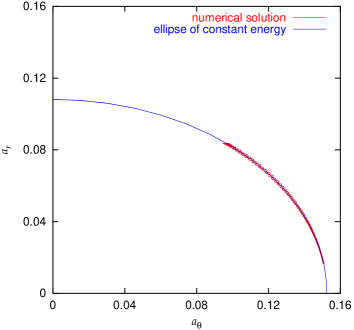
Figure 2: Comparison between an analytical constraint (71) and the corresponding numerical solution of the system Abramowicz et al., (2003). Each point corresponds to the amplitudes of the oscillations at a particular time. On the other hand, from the discussion of equation (71) we know that these points must lay on an ellipse, whose shape is determined by the multiple-scales method.

Behavior of the system is described by three variables $a_{r}(t)$, $a_{\theta}(t)$ and $\gamma(t)$ and three first-order differential equations (61), (62) and (63). However, the number of differential equations can be reduced to one because it is possible two find two integrals of motion of the system. Our discussion will be analogical to case of $1:2$ resonance of systems with quadratic nonlinearity, as examined by Nayfeh & Mook, (1979).

Consider equations (61) and (62). Eliminating $\sin\gamma$ from both equations we find

$$\frac{d}{dt}(a_{r}^{2}+\nu a_{\theta}^{2})=0$$ (70)

and thus

$$a_{r}^{2}+\nu a_{\theta}^{2}=\mathrm{const}\equiv E,$$ (71)

where we defined

$$\nu=\frac{\alpha\omega_{r}}{\beta\omega_{\theta}}\approx\frac{2\alpha}{3\beta}.$$ (72)

When $\nu>0$, the both amplitudes of oscillations are bounded. The curve $[a_{r}(t),a_{\theta}(t)]$ is a segment of an ellipse. The constant $E$ is proportional to the energy of the system. On the other hand, when $\nu<0$, one amplitude of oscillations can grow without bounds while the second amplitude vanishes. This case corresponds to the presence of an regenerative element in the system (Nayfeh & Mook, 1979). The corresponding curve in the $(a_{r},a_{\theta})$ plane is a hyperbola. In further discussion we assume that $\nu>0$.

In order to verify that the the energy of the system is conserved, we numerically integrated governing equation (27) and (28) for the one particular system discussed by Abramowicz et al., (2003). The comparison is in figure 2. The numerical and analytical results are in very good agreement.

The second integral of motion is found in following way. Let us multiply the equation (63) by $a_{\theta}$. Then we obtain

$$a_{\theta}\dot{\gamma}=-\sigma a_{\theta}+\frac{\omega_{\theta}}{4}\mu_{r}a_{r}^{2}a_{\theta}+\frac{\omega_{\theta}}{4}\mu_{\theta}a_{\theta}^{3}+\frac{\omega_{\theta}}{8}\alpha a_{r}a_{\theta}^{3}\cos\gamma-\frac{\omega_{\theta}}{8}\beta a_{r}^{3}a_{\theta}\cos\gamma.$$ (73)

Changing the independent variable from $t$ to $a_{\theta}$ and multiplying the whole equation by $da_{\theta}$ we find

$$a_{r}^{3}a_{\theta}^{2}d(\cos\gamma)+\frac{8\sigma}{\beta\omega_{\theta}}d(a_{\theta}^{2})-\frac{4\mu_{r}}{\beta}a_{r}^{2}a_{\theta}d(a_{\theta}^{2})-\frac{\mu_{\theta}}{\beta}d(a_{\theta}^{4})-$$

$$-\frac{2\alpha}{\beta}a_{r}a_{\theta}^{3}\cos\gamma da_{\theta}+2a_{r}^{3}a_{\theta}\cos\gamma da_{\theta}=0.$$ (74)

The equation (71) implies

$$a_{\theta}da_{\theta}=-\frac{a_{r}da_{r}}{\nu}.$$ (75)

With aid of this relation the equation (4.2) takes the form

$$3a_{r}^{2}a_{\theta}^{2}\cos\gamma da_{r}+2a_{r}^{3}a_{\theta}\cos\gamma da_{\theta}+a_{r}^{3}a_{\theta}^{2}d(\cos\gamma)+$$

$$+\frac{8\sigma}{\beta\omega_{\theta}}d(a_{\theta}^{2})+\frac{\mu_{r}}{\beta\nu}d(a_{r}^{4})-\frac{\mu_{\theta}}{\beta}d(a_{\theta}^{4})=0.$$ (76)

The first three terms express the total differential of function $-a_{r}^{3}a_{\theta}^{2}\cos\gamma$. Hence, the above equation can be arranged to the form

$$d\left(a_{r}^{3}a_{\theta}^{2}\cos\gamma+\frac{8\sigma}{\beta\omega_{\theta}}a_{\theta}^{2}+\frac{\mu_{r}}{\beta\nu}a_{r}^{4}-\frac{\mu_{\theta}}{\beta}a_{\theta}^{4}\right)=0.$$ (77)

In other words,

$$a_{r}^{3}a_{\theta}^{2}\cos\gamma+\frac{8\sigma}{\beta\omega_{\theta}}a_{\theta}^{2}+\frac{\mu_{r}}{\beta\nu}a_{r}^{4}-\frac{\mu_{\theta}}{\beta}a_{\theta}^{4}=\mathrm{const}\equiv L$$ (78)

is another integral of equations (61)–(63).

4.3 Analytical results

Knowing two integrals of motion, we should be able to find one differential equation which governs behavior of the system.

First, the amplitudes $a_{r}$ and $a_{\theta}$ are not independent because they are related by equation (71). To satisfy this relation, let us define new variable $\xi(t)$ by

$$a_{r}^{2}=\xi E, a_{\theta}^{2}=(1-\xi)\frac{E}{\nu}.$$ (79)

The equation describing an evolution of $\xi(t)$ is derived as follows. Let us multiply equation (61) by $2a_{r}$ and integrate it. We obtain

$$\frac{d(a_{r}^{2})}{dt}=\frac{\alpha}{8}\omega_{r}a_{r}^{3}a_{\theta}^{2}\sin\gamma.$$ (80)

Then we express $a_{r}^{2}$ using $\xi$, and square it. We find

$$\left(\frac{8E}{\alpha\omega_{r}}\right)^{2}\dot{\xi}^{2}=\left(a_{r}^{3}a_{\theta}^{2}\sin\gamma\right)^{2}.$$ (81)

The right-hand side of this equation can be expressed using (78)

$$\left(a_{r}^{3}a_{\theta}^{2}\sin\gamma\right)^{2}=\left(a_{r}^{3}a_{\theta}^{2}\right)^{2}-\left(L-\frac{8\sigma}{\beta\omega_{\theta}}a_{\theta}^{2}-\frac{\mu_{r}}{\beta\nu}a_{r}^{4}+\frac{\mu_{\theta}}{\beta}a_{\theta}^{4}\right)^{2}.$$ (82)

After the substitution into the equation (81) and using the relations (79), we get

$$\frac{1}{E^{3}}\left(\frac{8}{\beta\omega_{\theta}}\right)^{2}\dot{\xi}^{2}=(1-\xi)^{2}\xi^{3}-\frac{\nu^{2}}{E^{5}}\left[L-\frac{8\sigma E}{\beta\nu\omega_{\theta}}(1-\xi)-\frac{\mu_{r}E^{2}}{\beta\nu}\xi^{2}+\frac{\mu_{\theta}E^{2}}{\beta\nu^{2}}(1-\xi)^{2}\right]^{2}.$$ (83)

The equation of motion has very familiar form

$$\mathcal{K}^{2}\dot{\xi}^{2}=F^{2}(\xi)-G^{2}(\xi),$$ (84)

where the $\mathcal{K}^{2}$ is a positive constant, $F(\xi)=(1-\xi)\xi^{3/2}$ and $G(\xi)$ is a quadratic function which coefficients depend on initial condition through $E$ and $L$. For example, the equation with an effective potential, which governs motion of test particle around a massive body, has the same form. Therefore the following discussion is identical as in that case.

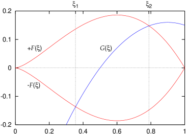
Figure 3: The functions $\pm F(\xi)=\pm(1-\xi)\xi^{3/2}$ and the quadratic function $G(\xi)$ which second powers are first and second terms on the right-hand side of the equation (83). The behavior of the system corresponds to $\xi$ in the interval $[\xi_{1},\xi_{2}]$ (denoted by the two dotted vertical lines) where the condition $|F(\xi)|\geq|G(\xi)|$ is satisfied.

In general, the motion occurs only when $\dot{\xi}^{2}$ is positive and thus for $\xi$ which satisfy $|F(\xi)|\geq|G(\xi)|$. The turning points, where $\dot{\xi}$ changes its signature, are determined by the condition

$$|F(\xi)|=|G(\xi)|.$$ (85)

The functions $\pm F(\xi)$ and $G(\xi)$ are plotted in figure 3. Generally, the function $G$ intersects functions $\pm F$ in two points which corresponds to $\xi(t)$ oscillating between two bounds $\xi_{1}$ and $\xi_{2}$ given by condition (85). In that case the radial and vertical mode of oscillations will periodically exchange the energy. The exchanged energy is given by $\Delta E/E=\xi_{2}-\xi_{1}$. However, for some particular values of $L$ and $E$ only one intersection of $\pm F$ and $G$ can be found. These stationary oscillations correspond to the steady-state solutions discussed above.

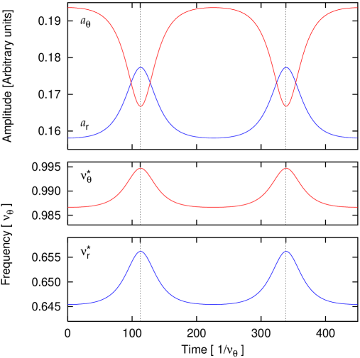
Figure 4: Time evolution of the amplitudes (top panel) and the observed frequencies, $\nu_{\theta}^{\star}=\omega^{\star}_{\theta}/(2\pi)$ (middle panel) and $\nu_{r}^{\star}=\omega^{\star}_{r}/(2\pi)$ (bottom panel). All quantities are rescaled with respect the higher eigenfrequency $\nu_{\theta}$. Amplitudes of the oscillations are anticorrelated because the energy is conserved. Observed frequencies are correlated because the system is in parametric resonance.

The period of the energy exchange can be find by integration of the equation (83)

$$T=\frac{16}{\beta\omega_{\theta}}E^{-3/2}\int_{\xi_{1}}^{\xi_{2}}\frac{d\xi}{\sqrt{F^{2}(\xi)-G^{2}(\xi)}}.$$ (86)

The integral on the right-hand side can be estimated in the following way. Since $P_{5}=F^{2}(\xi)-G^{2}(\xi)$ is a polynomial of the fifth order in $\xi$ having two roots $\xi_{1}$ and $\xi_{2}$ in the interval $[0,1]$, we can write it as $-(\xi-\xi_{1})(\xi-\xi_{2})P_{3}(\xi)$, where $P_{3}(\xi)$ is a polynomial of the third order positive in the interval $[0,1]$. Using the mean-value theorem we get

$$\int_{\xi_{1}}^{\xi_{2}}\frac{d\xi}{\sqrt{-(\xi-\xi_{1})(\xi-\xi_{2})P_{3}(\xi)}}=\frac{1}{p}\int_{\xi_{1}}^{\xi_{2}}\frac{d\xi}{\sqrt{-(\xi-\xi_{1})(\xi-\xi_{2})}}=\frac{\pi}{p},$$ (87)

where $p>0$ is a value of $P_{3}$ for some $\xi$ in the interval $[\xi_{1},\xi_{2}]$. Since $P_{5}\sim F^{2}\sim 0.01$ and $(\xi_{2}-\xi_{1})^{2}\sim 0.01$ typically, the values of $P_{3}(\xi)$ are of order of unity, and therefore $p\sim 1$. The period of the energy exchange can be roughly approximated by

$$T\sim\frac{16\pi}{\beta\omega_{\theta}}E^{-3/2}.$$ (88)

However, near the steady state $(\xi_{2}-\xi_{1})^{2}$ approaches to zero and the period becomes much longer.

The observed frequencies $\omega^{\star}_{r}$ and $\omega^{\star}_{\theta}$, given by relations (69), depend on squares of amplitudes $a_{r}$ and $a_{\theta}$. Since both $a_{r}^{2}$ and $a_{\theta}^{2}$ depend linearly on $\xi(t)$, also observed frequencies are linear functions of $\xi$ and are linearly correlated. The slope of this correlation $\omega^{\star}_{\theta}=K\omega^{\star}_{r}+Q$ is independent of the energy of oscillations and is given only by parameters of the system,

$$K=\frac{\omega_{\theta}}{\omega_{r}}\frac{\lambda_{r}\nu-\lambda_{\theta}}{\kappa_{r}\nu-\kappa_{\theta}}.$$ (89)

The slope of the correlation differs from $3:2$, however the observed frequencies are still close to it.

4.4 Numerical results

The equations (61)–(63) were solved numerically using the fifth-order Runge-Kutta method with an adaptive step size. One of the solutions is shown in figure 4. The top panel of the figure 4 shows the time behavior of the amplitudes of two modes of oscillations. Since energy of the system is constant, amplitudes are anticorrelated and the two modes are continuously exchanging energy between each other. The middle and the bottom panels show the two observed frequencies that are mutually correlated. They are also correlated to one of the amplitudes. The frequency ratio varies with time and it differs from the exact $3:2$ ratio, however, it always remains very close to it. The numerical solution is in agreement with the general results obtained analytically in the previous section.

5 Conclusions

Although this paper was originally motivated by observations and models connected to high-frequency QPOs, our results are very general and can be applied to any system with governing equations of the form (27) and (28). Moreover, the solvability conditions, which are derived for all resonances up to the fourth order and summarized in tables 1, 2 and 3, are valid also for non-conservative systems. In the latter case, the only difference is that constants $C^{(n,x)}_{\alpha}$ that appear in the multiple scale expansion are generally complex. However, the results discussed in section 4 were derived under the assumption that the system is conservative and thus all the constants $C^{(n,x)}_{\alpha}$ are real.

The main result of this calculation is the prediction of low-frequency modulation of the amplitudes and frequencies of oscillations. The characteristic timescale is approximately given by equation (88). In a separate paper by Horák et al., (2004) we pointed to possible connection of this modulation with the ‘normal branch oscillations’ (NBOs) that are often present together with QPOs. Specifically, we suggest that the correlation between the higher frequency and the lower amplitude, evident in figure 4, is the same as was recently reported in Sco X-1 by Yu et al., (2001).

It is a pleasure to thank Vladimír Karas, Marek Abramowicz, Wlodek Kluźniak, Paola Rebusco, Michal Bursa and Michal Dovčiak for helpful discussions. This work was supported by the GACR grant 205/03/0902 and GAUK grant 299/2004.

References

- Abramowicz et al., (2002) Abramowicz M.A., Bulik T., Bursa M., Kluźniak W., 2002, A&A, 404, L21
- Abramowicz et al., (2003) Abramowicz M.A., Karas V., Kluźniak W., Lee W.H., Rebusco P., 2003, PASJ, 55, 467
- Abramowicz & Kluźniak, (2001) Abramowicz M.A., Kluźniak W., 2001, A&A, 374, L19
- Abramowicz & Kluźniak, (2003) Abramowicz M.A., Kluźniak W., 2003, GReGr, 35, 69
- Abramowicz et al., (2004) Abramowicz M.A., Kluźniak W., Stuchlík S., Török G., 2004, astro-ph/0401464
- Horák et al., (2004) Horák J., Abramowicz M.A., Karas V., Kluźniak W., 2004, PASJ, in press
- Karas, (1999) Karas V., 1999, PASJ, 51, 317
- Kato, (2003) Kato S., 2003, PASJ, 55, 801
- Kato, (2004) Kato S., 2004, PASJ, 56, 559
- Kluźniak & Abramowicz, (2000) Kluźniak W., Abramowicz M.A., 2001, Acta Phys. Pol. B, B32, 3605
- Lai, (1999) Lai D., 1999, ApJ, 524, 1030
- Li & Narayan, (2004) Li Li-Xin, Narayan R., 2004, ApJ, 601, 414
- Nayfeh, (1973) Nayfeh A.H., 1973, ‘Perturbation methods’ (John Wiley & sons, New York)
- Nayfeh & Mook, (1979) Nayfeh A.H., Mook D.T., 1979, ‘Nonlinear oscillations’ (John Wiley & sons, New York)
- Rebusco, (2004) Rebusco P., 2004, PASJ, 56, 553
- Remillard et al., (2002) Remillard R.A., Muno M.P., McClintock J.E., Orosz J.A., 2002, ApJ, 580, 1030
- Rezzola et al., (2003) Rezzolla L., Yoshida S’i., Zanotti O., 2003, MNRAS, 344, 978
- Schnittman & Bertchinger, (2004) Schnittman J.D., Bertschinger E., 2004, ApJ, 606, 1098
- Titarchuk, (2002) Titarchuk L., 2002, ApJ, 578, L71
- Yu et al., (2001) Yu W., van der Klis M., Jonker P.G., 2001, ApJ, 559, L29