Star count analysis of the interstellar matter in the region of L1251

We studied the ISM distribution in and around the star forming cloud L1251 with optical star counts. A careful calculation with a maximum likelihood based statistical approach resulted in B, V, R, I extinction distributions from the star count maps. A distance of $330\pm 30$pc was derived. The extinction maps revealed an elongated dense cloud with a bow shock at its eastern side. We estimated a Mach number of $M\approx 2$ for the bow shock. A variation of the apparent dust properties is detected, i.e. the $R_{V}=A_{V}/E_{B-V}$ total to selective extinction ratio varies from 3 to 5.5, peaking at the densest part of L1251. The spatial structure of the head of L1251 is well modelled with a Schuster-sphere (i.e. n=5 polytropic sphere). The observed radial distribution of mass fits the model with high accuracy out to 2.5pc distance from the assumed center. Unexpectedly, the distribution of $NH_{3}$ 1.3 cm line widths is also well matched by the Schuster solution even in the tail of the cloud. Since the elongated head-tail structure of L1251 is far from the spherical symmetry the good fit of the linewidths in the tail makes it reasonable to assume that the present cloud structure has been formed by isothermal contraction.

1 Introduction

The Cepheus Flare is an extended complex of molecular clouds, where luminous stars are clearly absent, and it harbors dark clouds forming low mass stars (for details see the comprehensive study of Kun (1998) on this region). L1251 ($\alpha_{2000}=22^{h}36^{m}\!\!.1;\delta_{2000}=+75\degr 16\arcmin$) is a dark cloud in this region at a distance of $300\pm 50pc$ (Kun & Prusti 1993) and apparently belongs to this complex. Already at the advent of molecular radio astronomical studies in the late sixties the cloud was detected among the ten brightest OH emission sources on the sky by Cudaback & Heiles (1969). The cloud was also listed among sources of strong formaldehyde emission (Dieter 1973; Sume et al. 1975).

After these early successes of molecular radio observations L1251 apparently escaped the attention of radio observers. Although Kun (1982) discovered a number of $H\alpha$ emission stars associated with L1251, only appeared again in molecular radio studies in the late eighties (Sato & Fukui 1989; Zhou et al. 1989; Benson & Myers 1989). Zhou et al. (1989) recognized an ammonia core in the dense part of the cloud and comparing the large number of $H\alpha$ objects associated with the cloud, Sato & Fukui (1989) concluded that the star formation efficiency is anomalously high in L1251. From all of these facts it was obvious that the star formation processes in this region needed further detailed investigations. This motivated Kun & Prusti (1993) to study the properties and distribution of faint IRAS point sources along with the $H\alpha$ emission objects. Their study indicated that L1251 has been forming low-mass stars with an efficiency higher than usually encountered in dark clouds. The eastern, head region of the cloud has been found to contain more evolved YSOs than the western (tail) side.

A census of dense cores carried out by Tóth & Walmsley (1996) based on the $NH_{3}$ 1.3 cm line using the 100 m dish at Effelsberg resulted in detection of eight ammonia cores with typical size of $FWHM\approx 2\arcmin$ (0.2pc at 350pc distance). Five of the cores were found to be gravitationally bound. L1251 was recently surveyed in several mm lines, the structure and kinematics of the cores were studied e.g. by Caselli et al. (2002), Lee et al. (1999), Lee et al. (2001) and Nikolić et al. (2003). Both infall and outward motions were detected in the gravitationally unstable cores.

Tóth et al. (1995) tried to explain the shape of the cloud, as seen in the CO observations (Goodman et al. 1993; Sato et al. 1994), by hydrodynamical modelling assuming an encounter of a dense molecular cloud with an external shock, probably originating from a nearby supernova explosion. The reality of this assumption is supported by the detection of a soft X-ray excess region east of the cloud by Grenier et al. (1989). Further confirmation of an SN explosion comes from the space motion of the runaway star HD203854 (Kun et al. 2000).

Although the dense gas component of the cloud is well studied, much less is known about the distribution and properties of interstellar dust in and around L1251. Recently Kandori et al. (2003) studied the extinction of the dust component using B, V, R, I star counts and found high $R_{V}$ values indicating grain growth in the head of the cloud.

In the present paper we study the spatial distribution of dust, the mass, and the basic physical properties in the cloud by means of new optical extinction maps in B, V, R, I colors. In a subsequent paper the thermal emission of the dust grains in the dense regions of the cloud will be analyzed on the basis of far-infrared (120 and 200$\mu m$) maps obtained from the Infrared Space Observatory (Tóth et al. in prep.). The two complementary studies will clarify the spatial distribution of dust with respect to the distribution of the dense gas, and indicate how the star formation activity and the encounter with the external shock has modified the properties of the dust particles. To obtain direct information on the spatial distribution of dusty material the study of star counts is still one of the most reliable approaches. The basic aim of this paper is to carry out such analysis.

2 Input data

To study the surface distribution of the optical extinction we obtained star counts in B, V, R, I colors based on photographic observations with the 60/90/180 cm Schmidt telescope of the Konkoly Observatory. The plates were digitized with a pixel size of 20 microns in a $1.5\times 1.5$ degree field around L1251 using the PDS microdensitometer of the Vienna Observatory in 1991. We scanned 4, 3, 3, and 2 plates in $B,V,R_{J},I_{J}$ colors, respectively. The scans were processed with the ROMAPHOT photometric programme integrated into the MIDAS data analysis package. The plates were calibrated via CCD observations performed with the 1.23 m Ritchey-Chretien telescope of the German-Spanish Observatory, Calar Alto (Balázs et al. 1992). The limiting magnitude of the photographic survey was 19.0, 18.5, 17.5, and 16.5 in $B,V,R_{J},$ and $I_{J}$, respectively. Although these figures are less than could be obtained from the Digitized Sky Survey maps (see e.g. the extinction maps of Cambrésy (1999)), the well defined color system, the much better photometric calibration and four colors, however, support using our data. The estimated completeness of star counts was about 1.5 magnitude above the detection limit of the plates. The final star count maps of the region were obtained by counting the stars in each color on pixels of $6\arcmin\times 6\arcmin$ size and a $2\arcmin$ mesh of the star count maps was selected in both directions. (This resolution approximately corresponds to those of the 100 $\mu m$ IRAS maps). Kun (1982) and Kun & Prusti (1993) lists 12 $H\alpha$ objects (candidate pre-main sequence stars) apparently associated with the cloud. Their effect on the $R$ and $I$ star counts might be significant. Consequently, we have omitted them from further analysis.

3 Extinction maps from star counts

Several studies indicated empirically that the surface distribution of star counts is an excellent tracer of optical extinction. (e.g. Dickman (1978); Cernicharo et al. (1985)). This means that there is a simple linear relationship between the logarithmic star counts and the $a_{cl}$ extinction of a dust cloud:

$$a_{cl}=a\times\log(N(m))+b(m)$$ (1)

where $N(m)$ is the cumulative star count up to a given $m$ limiting magnitude, the $a$ constant and $b(m)$ depend on the Galactic longitude and latitude; $-b/a=\log(N_{0}(m))$ measures the logarithmic star count in an extinction-free region (Dickman 1978).

In the following we calibrate this expression using a multivariate statistical method, the $k$-means clustering, and a maximum likelihood procedure. Based on this calibrated relationship we assign extinction values to each star count pixel yielding an extinction map of the cloud. The procedure gives as a byproduct the distance of L1251 which enables us to calculate the mass of the cloud. Since we derive the extinction of the cloud in different colors we also discuss the ratio of the selective to total extinction.

3.1 Definition of areas of similar extinction

The B, V, R, I star count data on the pixels defined above represent a distribution of points in a four dimensional B, V, R, I parameter space. Following the relationships between star counts and extinction we assumed that the regions of equal extinction have equal star counts on the maps. In other words, looking for areas of equal extinction means searching for points of similar coordinates, i.e. lying close to each other in the four dimensional parameter space, made up of the pixel values of the star count maps.

The linear relationship between the logarithmic star counts and interstellar extinction predicts a one dimensional manifold in the four dimensional parameter space, stretched by the extinction, and there is a Poisson noise superimposed on it by the star counts. Therefore, to convert star counts into optical extinction we had to divide the whole star count map into regions of equal counts. According to Equation (1) the logarithms of the star counts scale linearly with the extinction; therefore we used the logarithmic B, V, R, I star counts in this procedure.

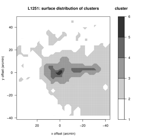
Figure 1: Result of the clustering, reprojected onto the celestial sphere. The areas of same grey level represent pixels in the map belonging to the same cluster and have similar extinction. We displayed the cloud in rectangular coordinates in a plane tangential to the celestial sphere. North is at the top and East is to the left. The (0,0) position corresponds to $\alpha_{2000}=22^{h}36^{m}\!\!.1;\,\delta_{2000}=+75\degr 16\arcmin$.

In order to divide the points into groups of similar extinction in the parameter space we invoked the technique of $k$-means clustering (see e.g. Murtagh & Heck (1987)). K-means clustering orders the points in the parameter space into $k$ groups. The $k$ number of the groups should be specified before running the clustering procedure. Assigning the points to any of the groups proceeds on the basis of some distance measure between the points. We used squared Euclidean distance.

There are no definite criteria for fixing the value of $k$. By trial we selected $k=5$ enabling clear separation of the high extinction regions from those of low extinction and ensuring enough stars in each cluster for reliable analysis. Figure 1 shows the result of the clustering, reprojected onto the celestial sphere. Areas of same grey level in the map represent pixels belonging to the same cluster and consequently, having similar extinction. Table  1 summarizes the number of stars in each subregion (cluster) in each color. One can infer from the data of this table that the 5th cluster is scarcely populated, therefore we excluded it from further analysis.

Table 1: Summary of the star count analysis of L1251, number of stars in each cluster and in each color

$FIELD$	$AREA(SqD)$	$N_{B}$	$N_{V}$	$N_{R}$	$N_{I}$
1.	0.9880	3982	3929	3939	2723
2.	0.8770	1883	2045	2186	1530
3.	0.1515	101	143	146	138
4.	0.0605	7	13	14	15
5.	0.0090	1	2	4	4

The central, densest part of L1251 is clearly separated from the surrounding lower extinction region. It resembles a bullet moving at supersonic speed with respect to the ambient medium. The less dense area surrounding the bullet-like main body of the cloud has a form of a bow shock. Accepting this view one can estimate the speed of the cloud relative to the ambient medium. The interaction of the cloud with its surroundings is probably the key issue in understanding the history of star formation. We will return to this problem in Sect. 4.

3.2 Modelling the effect of extinction on the star counts

3.2.1 Modelling differential star counts

To calibrate star counts in terms of optical extinction we attempted to model the observed apparent magnitude distribution of the stars. The starting point of our approach was the Galactic model of Wainscoat et al. (1992). Following the basic ideas of this model we assumed that the spatial distribution of the stars in the region investigated can be satisfactorily described by superposition of exponential disks, corresponding to different types of stars, and a spheroidal component. The exponential disks were defined by their scale heights and local stellar densities near the Sun. We used the data of Wainscoat et al. (1992) for the characteristic values of the exponential disks in the model.

To model the effect of the absorbing cloud on the star counts we assumed that besides the obscuring matter associated with L1251 there is no other significant dust cloud in the line of sight. This assumption is quite reasonable due to the high ($+15\degr$) galactic latitude of L1251. As in the Wainscoat et al. (1992) model we assumed that the diffuse component of interstellar extinction has the form

$$a_{diff}(r)=a_{0}\sec(b)(1-\exp(-r\sin(b)/h))$$ (2)

where $a_{0}$ is a constant depending on the color selected, $b$ is the Galactic latitude of the cloud and $h$ is the scale height of the obscuring material. We added to the extinction described above a further component in the form of a step function.

$$a(r)=a_{diff}(r)+a_{cl}(r);\quad a_{cl}(r)=\cases{0,&if $r<r_{cl}$\cr a_{cl},&if $r>r_{cl}$}$$ (3)

The distance of the cloud, $r_{cl}$, and the cloud extinction, $a_{cl}$, are constants to be estimated within a cluster obtained by the k-means clustering in the star count parameter space.

3.2.2 Maximum likelihood estimation of the distance and extinction

The model described in the previous section allows us to get the distance and extinction of the cloud using the maximum likelihood (ML) estimation. According to our model assumption the probability density of the apparent magnitude of stars in our observed sample is given by

$$A(m|a_{cl},r_{cl})=$$ (4)

$$\omega\sum_{sp}\int_{0}^{\infty}D_{sp}(r)\Phi(m-5\log(r)-5-a(r|a_{cl},r_{cl}))r^{2}dr$$

In the above formula $\omega$ is a suitably chosen normalizing constant, $D_{sp}(r)$ is spatial density, $\Phi$ is the luminosity function assumed to have a Gaussian form and $sp$ runs over the spectral types represented in the Wainscoat et al. (1992) model. We used a Monte Carlo simulation to get a distribution of apparent magnitudes corresponding to the probability density of $A(m|a_{cl},r_{cl})$. We used the MC simulated data to calculate the numerical values of $A$ for the ML procedure.

The likelihood function in our case can be written as

$$L(a_{cl},r_{cl})=\sum_{i=1}^{n}\log(A(m_{i}|a_{cl},r_{cl}))$$ (5)

where $m_{i}$-s are the observed apparent magnitudes in one of the colors in our sample. Maximization of $L(a_{cl},r_{cl})$ with respect to $a_{cl}$ and $r_{cl}$ yields the ML estimation of the extinction and the distance of the cloud.

Table 2: Summary of the star count analysis of L1251, extinction

$FIELD$	$AREA(SqD)$	$a_{B}$	$\sigma_{a_{B}}$	$a_{V}$	$\sigma_{a_{V}}$	$a_{R}$	$\sigma_{a_{R}}$	$a_{I}$	$\sigma_{a_{I}}$
1.	0.9980	0.45	0.05	0.30	0.05	0.12	0.05	0.10	0.03
2.	0.8770	1.55	0.10	1.25	0.07	0.85	0.07	0.63	0.07
3.	0.1515	3.30	0.15	2.65	0.15	2.20	0.15	1.75	0.2
4.	0.0605	6.5	0.80	5.2	0.80	$>5.3$	-	4.5	0.4

Performing the ML estimation within all groups given by the $k$-means clustering and in all colors separately, we obtained the results summarized in Tables 2 and 3. The results summarized in Table 2 enable us to convert the star counts in different colors into extinction. We return to this calibration in the following subsection.

Table 3: Summary of the star count analysis of L1251, distance moduli; the weighted mean of the data gives $7.58\pm 0.2$

$FIELD$	$AREA(SqD)$	$r_{B}$	$\sigma_{r_{B}}$	$r_{V}$	$\sigma_{r_{V}}$	$r_{R}$	$\sigma_{r_{R}}$	$r_{I}$	$\sigma_{r_{I}}$
1.	0.9880	7.45	0.60	$>$8.50	-	-	-	-	-
2.	0.8770	7.50	0.35	7.75	0.55	$<$7.6	-	$<$7.4	-
3.	0.1515	7.75	0.30	7.65	0.45	7.65	0.45	$<$7.4	-
4.	0.0605	7.05	0.7	$<$7.4	-	$<$7.4	-	$<$7.3	-

One may use the calculated distance moduli in Table 3 to get an estimate for the distance of L1251. We computed a weighted mean of the data in the table using weights inversely proportional to $\sigma$. It resulted in a distance modulus of $7.58\pm 0.2$ corresponding to $330\pm 30$ pc.

3.2.3 Confidence interval for the parameters estimated

The ML estimation provides a straightforward way to obtain the confidence interval for the estimated parameters, the extinction and distance. Denoting the value of the parameters maximizing the likelihood function with $a_{cl}^{max}$, $r_{cl}^{max}$ and with $a_{cl}^{true}$ , $r_{cl}^{true}$ their true values we have asymptotically, if the sample size goes to infinity,

$$2[L(a_{cl}^{max},r_{cl}^{max})-L(a_{cl}^{true},r_{cl}^{true})]=\chi^{2}_{k};\quad k=2$$ (6)

In general, k equals the number of parameters estimated and $\chi^{2}_{k}$ is a $\chi$-square variable with k degrees of freedom (for the proof of this theorem see Kendall & Stuart (1976, 1979)). The probability that the true values of the parameters are within a certain region in the k dimensional parameter space is given by

$$P(\chi^{2}_{k}\leq{\chi_{0}^{2}}_{k})=1-\delta$$ (7)

The projection of this k dimensional domain which is given by the $\chi^{2}_{k}\leq{\chi_{0}^{2}}_{k}$ inequality yields the confidence interval of the individual parameter values estimated by the ML procedure. The ${\chi_{0}^{2}}_{k},\delta$ pairs are tabulated in the literature (see e.g Kendall & Stuart (1976, 1979)). The confidence intervals corresponding to the $1\sigma$ levels are given in the $\sigma$ columns of the tables. In the case of $Field$ 4, due to the small numbers of stars the confidence interval is not closed towards higher extinctions and lower distances.

3.3 Star count - extinction conversion

3.3.1 Verifying the linear $\log N(m)$ - extinction relationship

The results yielded by the ML analysis enabled us to verify the star count - extinction relationship in each color in our study. Assuming the functional form of the formula given by Eq. (1) one can get its constants by a linear least squares fitting of the star counts versus extinction given in Table 2. We summarized the results of the least squares fitting in Table 4.

Table 4: Linear least squares fitting of the $a_{cl}=a\times\log(N(m))+b(m)$ extinction - star count relation

$color$	$a$	$\sigma_{a}$	$b(m)$	$\sigma_{b}$
$B$	$-$4.08	0.23	5.78	0.21
$V$	$-$4.08	0.16	5.67	0.15
$R$	$-$4.39	0.30	5.86	0.28
$I$	$-$4.52	0.18	5.31	0.16

Table 4 clearly demonstrates that the linear relationship fits the data obtained from the ML analysis. This means that the postulated linearity was convincingly recovered from the ML analysis performed.

In the $B$ and $V$ colors the slope of the relationship is the same while in $R$ and in $I$, in particular, it significantly differs. In the literature the inverse value of $a$ is usually given. Using the value of $a$ obtained for $B$ would give a bias of about $0.44\,\log[N_{0}(m)/N(m)]$ $mag$ in the estimation of the optical extinction, in the $I$ color.

3.4 Surface distribution of the obscuring material

Based on the calibration procedure one may assign extinction to each pixel in the star count maps, in all of the four colors studied. Fig. 2 shows the contour maps of the extinction obtained in this way. The main body of the cloud stands out with a contrast of several magnitudes from the less obscured region behind the bow shock.

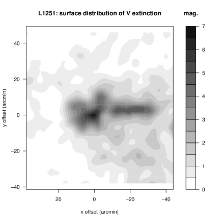
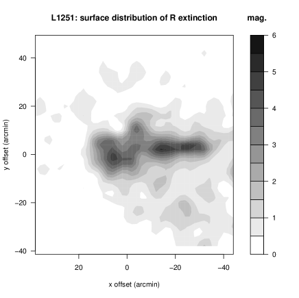
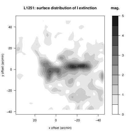
Figure 2: Contour maps of the extinction in the $B,V,R$ and $I$ color. The ‘flying bullet’ form of the main body and the bow shock displayed in Fig. 1 is clearly visible. The coordinates of the (0,0) position are same as in Fig. 1.

The overall distribution of the obscuring material, obtained from our study and that of Kandori et al. (2003), has a reasonably good correlation. There are, however, remarkable differences between them, in particular in the densest part of the cloud. The probable reason for these discrepancies lies in the different ways used in obtaining extinction maps from the surface distribution of the stars in the region of L1251. Both studies had a mesh of 2’ resolution but applied different kind of smoothing. We used a boxcar of 6’x 6’ size while the other study was a Gaussian filtering of 6’ resolution. It is probably important to note that the tails of the Gaussian filter give contributions from much wider areas, in particular in the densest part where the star counts have low values.

A further reason for the discrepancy might originate from the method of converting the star count maps into extinction. Our method accounts for the foreground stars whose contribution increases the counts and decreases correspondingly the estimated extinction values. We made simulations of the Wainscoat et al. (1992) model assuming a limiting magnitude of about 19 mag and 6 mag of extinction at the distance of L1251. The conventional method of star count extinction conversion resulted only in a 5 mag. value, i.e. one magnitude less than the true (6 mag.) extinction.

4 Discussion

4.1 Shape of the cloud

We have already indicated above that the extinction map derived from the star counts resembles a body flying at hypersonic speed across an ambient medium.

The shape of L1251 was accounted by Tóth et al. (1995) for a shock wave passing the cloud and produced by a nearby supernova. They showed that the cooling by the $H_{2}$ molecules plays an important role in the formation of the observable shape of the cloud.

The presence of a bow shock as indicated by the extinction maps suggests another type of cloud-environment interactions. The blunt body solutions of hypersonic flows are standard topics in textbooks (see e.g. Hayes & Probstein (1959). For the astrophysical context of the problem see the works of Rózyczka & Tenorio-Tagle (1985) and Canto & Raga (1998)). One can identify the tail of L1251 with a wake of the head of the cloud, typical of blunt body hypersonic streaming patterns.

In the following we do not try to fit the form of the bow shock using a solution of the blunt-body problem. This solution would allow a better understanding of the role of different significant physical parameters defining a particular fit, however this is beyond the scope of the present paper. An obvious significant parameter would be the Mach number of the flow which is easy to calculate from the angle between the two asymptotes of the bow shock (Hayes & Probstein 1959). The Mach number is given by $M=\sin(\alpha/2)^{-1}$ where $\alpha$ is the angle between the asymptotes. It yielded $M\approx 2$ in our case.

The symmetry axis of the bow shock has a tilt of about 10 deg to the main axis of L1251. The symmetry axis of the bow shock points toward the center of the bubble discovered by Grenier et al. (1989). Kun et al. (2000) found a runaway star which also might have been caused by the SN explosion that was probably responsible for the bubble and derived an age of $10^{6}$ yrs. According to this picture the bow shock resulted from an encounter of the cloud with the wind coming from the interior of the bubble.

4.2 Properties of the obscuring material

The estimation of the total extinction in different colors makes it possible to get the value of the total to selective extinction $R_{V}=a_{V}/E_{B-V}$ . The scatterplot between $a_{V}$ and $a_{B}$ is displayed in Fig. 3. The relationship between $a_{V}$ and $a_{B}$ can be written in the form of $a_{B}=(1+1/R_{V})\times a_{V}$. We marked with lines (labelled with the corresponding $R_{V}$ values) in Fig. 3 the relationships between $a_{V}$ and $a_{B}$ assuming that $R_{V}=3$ (close to the canonical value for the general interstellar matter) and $R_{V}=6$. The line assuming that the interstellar absorption does not depend on the color (grey approximation) is also marked with $R_{V}=inf$.

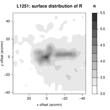
Figure 3: Scatterplot between $a_{V}$ and $a_{B}$ (left panel). The relationship between $a_{V}$ and $a_{B}$ can be written in the form of $a_{B}=(1+1/R)\times a_{V}$. We marked with lines (labelled with the corresponding $R$ values) the relationships between $a_{V}$ and $a_{B}$ assuming that $R=3$ (close to the canonical value for the general interstellar matter) and $R=6$. The line assuming that the interstellar extinction does not depend on the color (grey approximation) is also marked with $R=inf$. Assigning $R_{V}$ to each pixel we obtained a map of the total to selective extinction (right panel). One may infer from this map that the high values of $R_{V}$ are concentrated only in the densest parts of L1251. The coordinates of the (0,0) position are same as in Fig. 1.

Figure 3 clearly demonstrates that above $a_{V}=3$ (i.e. within the main central body of L1251) the points depart from the $R_{V}=3$ line and approach the lines of higher $R_{V}$ as one moves to higher extinction. Departure from the canonical $R_{V}=3.1$ towards higher values is a common behavior of dense clouds (see the review by Mathis (1990)).

Postulating a relationship in the form of $a_{B}=\alpha\times a_{V}$, where $\alpha=(1+1/R_{V})$, and substituting $R_{V}$ values between 3-6, we can infer that $\alpha$ depends only weakly on $a_{V}$ and may have approximately a form of $\alpha(a_{V})=\alpha_{0}+\alpha_{1}\times a_{V}$. Assuming that $R_{V}=1+1/\alpha_{0}=3.1$ we made a least squares fitting to get $\alpha_{1}$. In this way we obtained $R_{V}(a_{V})=1/(0.32-0.019\times a_{V})$ and $a_{B}=\alpha(a_{V})\times a_{V}$ gave a reasonably good fit to the points in Fig. 3.

Based on this result we may assign a value of $R_{V}$ to each pixel in the $a_{V}$ extinction map of L1251. We obtained a map of the total to selective extinction as given in Fig. 3. One may infer from this map that the high values of $R_{V}$ are concentrated only in the densest parts of L1251.

The canonical dependence of the interstellar extinction on the wavelength is realized by the standard relation of Savage & Mathis (1979) which can be well represented by a linear function of the extinction on $1/\lambda$ in the range of the B, V, R, I colors used in our study.

Departure from the standard $R_{V}=3.1$ value above $a_{V}=3$ in dense interstellar clouds, as we found in the case of L1251, was also obtained by Whittet et al. (2001) in the Taurus region. They claimed that for extinctions $a_{V}>3$ real changes in grain properties may occur, characterized by observed $R_{V}$ values in the range of 3.5-4.0. A simple model for the development of $R_{V}$ with $a_{V}$ suggested that $R_{V}$ may approach values of 4.5 or more in the densest regions of the cloud. According to Whittet et al. (2001) the transition between “normal” and “dense cloud” extinction occurs at $a_{V}\approx 3.2$, a value coincident with the threshold extinction above which $H_{2}O$-ice is detected on grains within the cloud.

The $R_{V}$ values derived in our analysis correspond to those obtained by Kandori et al. (2003) within the limits of the statistical errors. There are differences, however, in the surface maps between the two studies. To obtain $R_{V}$ values we used the relationship between the $a_{B}$ and $a_{V}$ values so our surface map reflects that of the extinction in the $V$ color. On the contrary, Kandori et al. (2003) applied an adaptive averaging of $B-V$ and $V-I$ color indices by varying the size of the smoothing window, keeping constant the number of stars in it but at the cost of the spatial resolution, in particular in the densest part of the cloud.

4.3 Mass of the cloud

Knowing the distance of L1251 we converted the $a_{V}$ extinction values into the mass using the empirical formula given by Dickman (1978). According to this formula

$$M=(\alpha d)^{2}\mu{N_{H}\over a_{V}}\sum_{i}a_{V}(i)$$ (8)

where $M,\alpha,d,\mu,a_{V}(i)$ are the mass of the cloud, the angular size of a pixel, the distance, the mean molecular mass and the extinction of a pixel, respectively; $N_{H}/a_{V}=1.87\times 10^{21}cm^{-2}mag^{-1}$ and $N_{H}=N_{HI}+2N_{H_{2}}$. Based on Dickman formula we computed the mass of the different subregions of the cloud as given in Table 5.

Table 5: Mass of the cloud (using the formula of Dickman (1978))

FIELD	AREA (SQD)	MASS ($M_{\odot}$)	NO. OF PIX.
1.	0.9880	153.34	887
2.	0.8770	490.48	784
3.	0.1515	212.60	136
4.	0.0601	132.05	54
5.	0.0089	26.07	8

Fields 3, 4 and 5 represent the main body of L1251. Based on Table 5 the total mass of this part of the cloud is 371 $M_{\odot}$. This value can be compared with the figure obtained by Sato et al. (1994) based on $C^{18}O$ measurements, taking into account that the field occupied by our main body lies completely inside the region covered by the $C^{18}O$ study and contains only 85 % of the mass calculated from it. Re-scaling this fraction of mass to the distance we obtained in this paper one gets 422$M_{\odot}$, surprisingly close to our estimated value. Studying a somewhat larger area than ours, Lee (1994) obtained $610\,M_{\odot}$ from his ${}^{12}CO$ and ${}^{13}CO$ measurements.

4.4 Mass model of the head of L1251

In the following we try to model the head of the cloud assuming spherical symmetry.

Figure 4: Fitting the radial distribution of the surface mass density by a Schuster sphere. Up to 2.5 pc distance from the center the fit is very good. Beyond this distance, however, there is an excess of the observed mass density due to the tail of the cloud.

Using the data obtained with VLT of the ESO Alves et al. (2001) modelled the spatial structure of the Bok globule Barnard 68. They supposed the globule to be an isothermal Bonnor-Ebert sphere (Bonnor 1956; Ebert 1955) in pressure equilibrium with the external, much hotter and less dense interstellar medium.

We have not required isothermality in our analysis. The isothermal solution is a specific case of the class of polytropic spheres studied extensively by Emden (1907). The isothermal solution represents the case when the polytropic index $n=\infty$. Actually, the mass of an isothermal sphere is infinite and the limit between the finite and infinite mass solutions is $n=5$. Although the mass is finite in this case the size of the sphere is infinite. One obtains finite size solutions only in the $n<5$ case. Recently, Medvedev & Rybicki (2001) studied the properties of polytropic spheres near $n=5$ and found them very suitable to characterize the structure of molecular cloud cores.

We fixed the mass center of the sphere at the maximum value of $a_{V}$. This choice is quite reasonable in view of Equation (8). We then averaged the $a_{V}$ values over concentric annuli. This procedure gave a radial profile of the extinction of the head of L1251. This profile can be converted into the surface mass density by Equation (8).

Evaluating the radial profile obtained from the observed data we projected the $n=5$ polytropic sphere (Schuster 1883) to get its surface mass density distribution. The Schuster sphere has two free parameters to be adjusted: the central mass density and a scale parameter. We get the fit displayed in Fig. 4. Up to 2.5pc distance from the center the fit is very good. Beyond this distance, however, there is an excess of the observed mass density due to the tail of the cloud which significantly distorts the spherical symmetry of the head.

The density parameter of the fitted Schuster sphere, $45M_{\odot}pc^{-3}$ ($3.06\times 10^{-21}{\rm gcm}^{-3}$), gives an estimate of the central mass density of the head of L1251. Comparing the finite size polytropic solutions of $n<5$ with those of the Schuster sphere (i.e. $n=5$) one can infer that they concentrate more mass at finite distances and give a much worse fit to the points observed.

Assuming a polytropic gas sphere one can compute the radial velocity dispersion profile from the fitted density profile, based on the polytropic equation of state. The $p/\rho$ ratio of the pressure and mass density gives the $T$ temperature, i.e. the velocity dispersion. The velocity dispersion projected onto the celestial sphere can be directly compared with that observed. The projected $FWHM$ of the V-profile of a Schuster sphere is displayed in Fig. 5, along with those of the $NH_{3}$ molecule measured by Tóth & Walmsley (1996).

There is a considerable scatter of the measured line widths in the head of the cloud around the mean which is well matched by the Schuster solution. The Schuster curve, however, gives an unexpectedly good fit in the tail region. This good fit is not expected far from the head since due to the tail the mass distribution drastically differs from the spherical symmetry. However, we may assume that our predicted FWHMs of the NH3 line refers to the initial stage and those measured by Tóth & Walmsley (1996) to the final stage of the formation of density enhancements in the tail region. We conclude therefore that the formation of structures in the tail left the linewidth practically unchanged. This indicates an isothermal contraction. However, the question remains open: what kind of instability played a significant role in forming the density enhancements in the tail? We note that according to Tóth & Walmsley (1996) the thermal energy is dominant over the turbulent energy in the NH3 cores of the tail region and thus we cannot exclude the scenario that thermal instability played a significant role in the cloud fragmentation.

Figure 5: $FWHM$ of the projected velocity profile of a Schuster sphere (dashed line) and the $NH_{3}$ molecule measured by Tóth & Walmsley (1996). There is a considerable scatter of the line widths in the head of the cloud around the mean which is well matched by the Schuster solution. The Schuster curve gives an unexpectedly good fit in the tail region.

5 Summary and conclusions

In this paper we studied the $B,V,R,I$ star count maps of L1251 to derive the spatial structure of the obscuring matter in the cloud. We assumed that the pixel values in the star count maps form a one dimensional manifold in the $BVRI$ four dimensional parameter space and defined areas of similar extinction by means of multivariate $k-means$ clustering. After defining areas of equal extinction we derived the amount of obscuration using a maximum likelihood procedure based on a Monte Carlo simulation of the Wainscoat et al. (1992) model. As a byproduct of the model fitting we obtained the $330\pm 30\,pc$ distance of the cloud.

The extinction maps clearly showed the main body of the cloud and a less dense region having a form of a bow shock of a blunt body. The form of the bow shock allowed us to calculate the approximate Mach number ($M\approx 2$) of the streaming around the head of L1251.

Comparing the obscuration of the dust in different colors we calculated the dependence of the total to selective extinction ($R_{V}$ value) on the visual extinction. The total to selective extinction exceeded $R_{V}=5$ in the densest part of the cloud.

Using Equation (8) to convert the optical extinction distribution into surface mass density we obtained the mass of 371 $M_{\odot}$ for the cloud, in reasonably good agreement with the 410 $M_{\odot}$ obtained by Sato et al. (1994), based on $C^{18}O$ measurements.

Assuming a spherical symmetry for the head of L1251 we computed the radial distribution of the mass and compared it with a polytropic model of $n=5$ (Schuster sphere). Up to $r=2.5\,pc$ from the center of the mass the fit is excellent but beyond this distance the observed points start to depart remarkably from the fit due to the drastic distortion of the spherical symmetry by the tail of L1251.

In the head of L1251 the Schuster model fit matches well the mean FWHM of the 1.3 cm NH3 line measured by Tóth & Walmsley (1996). It gives an unexpectedly good fit in the tail region indicating that isothermal contraction played a significant role in forming the density enhancements.