Prospects for ACT: simulations, power spectrum, and non-Gaussian analysis

Abstract

A new generation of instruments will reveal the microwave sky at high resolution. We focus on one of these, the Atacama Cosmology Telescope, which probes scales $1000<l<10000$, where both primary and secondary anisotropies are important. Including lensing, thermal and kinetic Sunyaev-Zeldovich (SZ) effects, and extragalactic point sources, we simulate the telescope’s observations of the CMB in three channels, then extract the power spectra of these components in a multifrequency analysis. We present results for various cases, differing in assumed knowledge of the contaminating point sources. We find that both radio and infrared point sources are important, but can be effectively eliminated from the power spectrum given three (or more) channels and a good understanding of their frequency dependence. However, improper treatment of the scatter in the point source frequency dependence relation may introduce a large systematic bias. Even if all thermal SZ and point source effects are eliminated, the kinetic SZ effect remains and corrupts measurements of the primordial slope and amplitude on small scales. We discuss the non-Gaussianity of the one-point probability distribution function as a way to constrain the kinetic SZ effect, and we develop a method for distinguishing this effect from the CMB in a window where they overlap. This method provides an independent constraint on the variance of the CMB in that window and is complementary to the power spectrum analysis.

1 Introduction

Several survey telescopes (SPT, APEX, ACT) will open a poorly probed regime of the microwave background: arcminute scales at frequencies up to a few hundred GHz. The sensitivities of these instruments will be a few micro-Kelvin. These efforts will provide a large amount of high-quality data, but face a different set of challenges than lower resolution surveys, such as WMAP. For lower resolution experiments the primary anisotropies of the CMB are the principal signal. The major contaminant is the galaxy, whose emission is diffuse and drops off rapidly away from the galactic center. By contrast, for higher resolution experiments, secondary anisotropies dominate at small scales. Assuming the observations are away from the galaxy at high frequencies, the major contaminant is extragalactic point source emission. For a wide range of interesting scales, point sources contribute substantially more power than the instrument noise.

The statistical properties of the primary CMB differ from those of these signals. Primary anisotropies, from the surface of last scattering, dominate the CMB on degree scales. The fluctuations are Gaussian, so the power spectrum sufficiently describes the anisotropy. Secondary anisotropies, such as lensing and the Sunyaev-Zeldovich (SZ) effect, depend on the late-time, nonlinear evolution of the universe. Their imprints need not be Gaussian.

In this work, we investigate the prospects of these experiments to extract the power spectrum and other statistical information for the components that contribute at these angular scales and frequencies. We are particularly interested in determining the primordial power spectrum from the primary CMB. Such a determination would enable one to determine the amplitude and slope of the fluctuations on small scales and, in combination with large scale observations, would allow one to place powerful constraints on models of structure formation. We model our investigations on the Atacama Cosmology Telescope (ACT), a 6 meter off-axis telescope to be placed in the Atacama desert in the mountains of northern Chile [1]. ACT’s bolometer array will measure in three bands from 145–265 GHz, with beams sized 1–2 arcminutes. (See Table 1.) ACT will survey about 100 square degrees of the sky with high signal to noise. In section 2, we simulate observations based on the specifications of ACT.

The first problem in extracting the primary CMB information from observations is separating the components on the sky with distinct frequency dependences. Although many signals at these scales are not Gaussian, the power spectrum is still the most important of the statistics, and in section 3 we extract the power spectrum with a multifrequency analysis. The power spectrum analysis requires knowledge of the frequency dependence of the signals and of the scatter in that relation. Our knowledge is presently incomplete, and any error biases the estimated power spectra. Our discussion explores the impact of estimating some of this frequency information from the data itself.

The second problem in extracting the primary CMB information is that one of the secondary anisotropies, the kinetic Sunyaev-Zeldovich (kSZ) effect (and its analogs like the Ostriker-Vishniac effect and patchy reionization effect), has the same frequency dependence as the primary CMB. This complicates their separation, requiring an explicit template for the kSZ power spectrum. Again our knowledge is incomplete, and any error biases the primary CMB power spectrum. We address in detail the impact of secondary anisotropies on the estimation of the amplitude and slope of primordial fluctuations.

Non-Gaussian information can help distinguish between the components which cannot be separated using frequency information. It is difficult to make non-Gaussian analysis fully exhaustive, so one must choose some simple statistics. Here we explore the one-point probability distribution function, in section 4. This can provide a consistency check on a kSZ template and can assist in signal separation. Finally, in section 5 we present our conclusions.

Band (GHz)	Beam FWHM (arcmin.)	Sensitivity per pixel ($\mu$K)
145	1.7	2
210	1.1	3.3
265	0.93	4.7

Table 1: Frequency channels, beam full-width at half maximum, and detector noise (thermodynamic temperature) of mock ACT survey.

2 Simulations

We simulate the sky as five astrophysical components (CMB, kSZ, SZ, and two types of point sources) plus noise. The CMB is a Gaussian random field. The density field (used for lensing of CMB), kSZ, and SZ are produced from hydrodynamical simulations [2]. Point sources are Poisson distributed from source count models. We add the appropriate detector noise and convolve with the telescope beam (assumed Gaussian).

We briefly examine the simulations in general, before addressing each signal in turn. The simulation contains forty fields, each $1.19^{\circ}\times 1.19^{\circ}$, totaling $\sim 57$ square degrees, somewhat smaller than the ACT survey. The results will therefore be appropriate for a smaller, more conservative mock survey. Throughout, we have used the following cosmological parameters in a flat, $\Lambda$CDM model: $\Omega_{c}=0.32$, $\Omega_{b}=0.05$, $\Omega_{\Lambda}=0.63$, $\sigma_{8}=1.0$, with $H_{0}=70$ km/s/Mpc.

We express our fields in temperature units, or as a temperature perturbation $\Theta(\hat{\mathbf{n}})=\Delta T(\hat{\mathbf{n}})/T_{\rm CMB}$ for line of sight $\hat{\mathbf{n}}$. Sample temperature perturbation maps of each signal are shown in Figure 1. We will refer to each image as we discuss the signals in greater detail. Signals which have a blackbody frequency dependence (CMB, kSZ) have the same temperature perturbation at all observed frequencies. For all other signals, the temperature perturbation will depend on the observation frequency.

In Fourier space, we use the flat sky approximation,

$$\Theta(\hat{\mathbf{n}})=\frac{1}{(2\pi)^{2}}\int d^{2}{\mathbf{l}}\ \Theta_{\mathbf{l}}\exp(i\hat{\mathbf{n}}\cdot{\mathbf{l}}).$$ (1)

The symbol $\mathbf{l}$ is a two dimensional wavevector. The power spectrum of a signal or channel is defined by $\langle\left|\Theta_{\mathbf{l}}\right|^{2}\rangle=C_{l}$. For each signal, figure 2 displays the power spectra and cross-correlations between the bands. Below we include a more detailed look at these spectra.

ACT will have channels near 145, 217, and 265 GHz, which in simulations we take to have delta function frequency responses. These bands are typical of ground based experiments because they lie in windows between atmospheric lines. The band at 217 GHz also takes advantage of the thermal SZ “null,” described below in section 2.3. Figure 3 show a simulated patch of sky observed by ACT in these three bands. We discuss this image further below.

In the next section, we discuss the hydrodynamical simulations which were the source of several of our signals. Then we study the signals and noise in more detail. Section 2.7 list caveats to our simulations. Section 2.8 summarizes the discussion of the simulations.

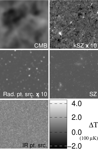
Figure 1: These simulated signals contribute to one of forty $1.2^{\circ}\times 1.2^{\circ}$ fields. All fields are in temperature units with a common gray scale, although kSZ and radio source signals have been multiplied by 10 for visibility. SZ is shown at $-T_{RJ}=2y$. The CMB, SZ, and kSZ are not convolved with any beam. For visibility, radio and infrared point sources are convolved with the beam of the channel in which are most prominent, respectively a 1.7 arcminute (145 GHz channel) and a 0.9 arcminute (265 GHz) full-width at half-maximum Gaussian beam.

2.1 Hydrodynamical simulations

Hydrodynamical simulations provide the density field for lensing, the SZ and kSZ effects. These simulations are described in more detail elsewhere [3, 4, 2, 5]. A 100 $h^{-1}$ Mpc periodic box was simulated at $512^{3}$ resolution with a moving mesh. At several redshift slices, the contents are projected onto a plane parallel to one of the box faces. These projections are stacked with random horizontal and vertical offsets to form maps which look back through a cone of the sky. The benefit to this method is that only one box must be simulated to create a much larger set of maps. In our case, we have forty maps from one simulation box. The obvious downside to this technique is that a single structure in the simulation may be seen several times, at different orientations and stages of development, in different fields. Thus the family of rare objects in the maps may not be truly representative.

We use the same simulations to obtain the convergence maps for CMB lensing, the comptonization parameter maps for thermal SZ, and $\Delta T/T$ maps for kinetic SZ. These are discussed below for each effect.

2.2 Lensed CMB

We employed CMBFAST [6] to generate the unlensed CMB power spectrum to $l=20\ 000$. This power spectrum was used to create a Gaussian random field, which is the unlensed CMB map. Lensing bends light from one part of the sky to another, so that the light observed from line-of-sight $\hat{\mathbf{n}}$ in reality came from $\hat{\mathbf{n}}+\delta\hat{\mathbf{n}}$. The real space displacement vector $\delta\hat{\mathbf{n}}$ may be calculated via the Fourier space relation, $\delta\hat{\mathbf{n}}(\mathbf{l})=2i\mathbf{l}\kappa(\mathbf{l})/l^{2}$. The convergence map for CMB lensing $\kappa(\hat{\mathbf{n}})$ is defined as a line-of-sight projection of the density perturbation $\delta\equiv\rho/\bar{\rho}-1$:

$$\kappa(\hat{\mathbf{n}})=\frac{3H_{0}^{2}\Omega_{m}}{2c^{2}}\int_{0}^{\chi_{\rm LS}}{r(\chi)r(\chi_{\rm LS}-\chi)\over r(\chi_{\rm LS})}{\delta({\mathbf{n}})\over a}d\chi.$$ (2)

The integral is over the comoving radial coordinate $\chi$. Here $\chi_{\rm LS}$ is the coordinate of the CMB’s surface of last scattering at recombination, the line element radial function $r(\chi)$ is simply $\chi$ for a flat universe, $\Omega_{m}$ is the matter density parameter, ${\mathbf{n}}$ describes position $(\hat{\mathbf{n}},\chi)$, and $a$ is the expansion factor of the universe. Software from [7] computes the lensed maps from unlensed maps and the convergence (See also [8]). Hydrodynamical simulations provided the convergence calculated from the gas density, $\delta_{g}$. Here we assume assume gas traces matter, which should be valid on scales of interest here. The primary CMB has Gaussian fluctuations, but lensing introduces non-Gaussianities by correlating the CMB with the nonlinear matter field.

A sample lensed CMB map is shown in Figure 1. The lensing has negligible visible effect on the maps. The CMB power spectrum is shown in Figure 2. Because we examine the temperature perturbation power spectrum, any signal with a blackbody frequency dependence will contribute equally in the three bands. This is the case for the CMB. Since the maps are only $1.2^{\circ}$ on a side the power spectrum bins have a width $\Delta l\approx 300$, so the acoustic peaks are not resolved. The CMB is the dominant signal on scales larger than $l\sim 1000$. The major features are the damping tail, where the power falls exponentially at $1000\mathrel{\hbox to0.0pt{\lower 4.0pt\hbox{\hskip 1.0pt$\sim$}\hss}\raise 1.0pt\hbox{$<$}}l\mathrel{\hbox to0.0pt{\lower 4.0pt\hbox{\hskip 1.0pt$\sim$}\hss}\raise 1.0pt\hbox{$<$}}4000$, and the contribution from lensing, which dominates the power at $l\mathrel{\hbox to0.0pt{\lower 4.0pt\hbox{\hskip 1.0pt$\sim$}\hss}\raise 1.0pt\hbox{$>$}}4000$.

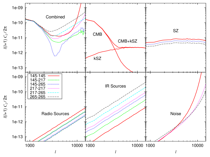
Figure 2: Auto- and cross-power spectra from the ACT bands, in bins of width $\Delta l\approx 300$. $C_{l}$ measures the power in temperature perturbation. Line type describes the frequency dependence of the signals. “145-145” denotes the power spectrum in the 145 GHz channel. “145-217” denotes the cross correlation between the 145 GHz and 217 GHz channels. Others correlations are labeled similarly. Each signal is depicted in a separate panel. ACT measures the sum of all signals and noise, shown in the panel marked “combined.” At each frequency in the combined signal, the CMB dominates at large scales. Small scales are dominated by experimental noise and infrared point sources. Effects with a Planck spectrum (CMB/kSZ) do not vary with frequency. The SZ 145 GHz-265 GHz cross correlation is negative, and is shown in absolute value.

2.3 Sunyaev-Zeldovich effect

The SZ (or thermal SZ) effect is a change in the spectrum of the CMB due to scattering off of hot gas in the potential wells of large structures (see [9, 10] for comprehensive reviews). Scattered CMB photons are preferentially raised in energy. This distorts the energy spectrum: in the direction of the hot gas, the CMB has fewer low-energy photons and more high-energy photons. The number of scatterings for a photon passing through a cluster is low, so the CMB photons do not achieve thermal equilibrium with the electrons. Therefore, the SZ effect does not follow a blackbody spectrum. If the electrons are not relativistic then the frequency dependence is

$$\Theta^{\rm SZ}(\hat{\mathbf{n}})=-2y(\hat{\mathbf{n}})\left[2-\frac{x/2}{\tanh(x/2)}\right],$$ (3)

where $x=h\nu/k_{B}T_{\rm CMB}$ and the comptonization parameter $y$ is given by the integral of the electron pressure along the line of sight:

$$y(\hat{\mathbf{n}})=\int\sigma_{T}n_{e}({\mathbf{n}}){k_{B}T_{e}({\mathbf{n}})\over m_{e}c^{2}}ad\chi.$$ (4)

Here $\sigma_{T}$ is the Thomson scattering cross section, $n_{e}$ is the electron density, and $T_{e}$ is the electron temperature. This expression is derived in the single scattering, non-relativistic limit. In the low frequency (Rayleigh-Jeans) regime, $x\ll 1$ and $\Theta^{\rm SZ}=-2y$. At roughly 217 GHz, the SZ effect is absent. This is known as the SZ null. At frequencies lower than the null, the spectrum is underpopulated relative to a blackbody, and the effect is seen as a temperature decrement. At higher frequencies, the spectrum is overpopulated, and the effect is a temperature increment. This very specific deviation from a thermal spectrum is SZ’s signature, and is vital for extracting the effect. At high electron temperatures, the formula for the frequency dependence needs relativistic corrections. These corrections in particular displace the SZ null. However, this effect has a minor impact for the application here: even if the electron temperature was increased everywhere to $T_{e}=20\ 000$ K (holding the $y$-parameter constant), the SZ power spectrum remains a minor addition to the 217 GHz band.

A sample SZ map, showing negative Rayleigh-Jeans temperature, is depicted in Figure 1. The SZ effect is most striking in clusters. The resulting signal is non-Gaussian.

The SZ effect has been studied extensively with simulations (e.g. [2, 11, 12, 4, 13, 14]) and semi-analytic methods [15, 16]. There are some differences in the results between different simulations and halo model predictions (see [15] for a discussion), but these are most prominent on very small scales, while in the relevant range around $l\sim 3000$ the agreement in the power spectrum is quite good. The SZ power spectrum from simulations used here [2] is shown in Figure 2. The effect of observation frequency is apparent. The SZ effect is most prominent, and negative, in the 145 GHz channel, absent at 217 GHz, and is substantial at 265 GHz. At very large scales, the discrete nature of clusters is apparent, and the power spectrum is like shot noise, with $C^{\rm SZ}_{l}$ constant. At smaller scales, the power goes as $C^{\rm SZ}_{l}\propto l^{-2}$ for scales of $2000\mathrel{\hbox to0.0pt{\lower 4.0pt\hbox{\hskip 1.0pt$\sim$}\hss}\raise 1.0pt\hbox{$<$}}l\mathrel{\hbox to0.0pt{\lower 4.0pt\hbox{\hskip 1.0pt$\sim$}\hss}\raise 1.0pt\hbox{$<$}}10000$. At yet higher $l$, the power falls faster.

2.4 Kinetic Sunyaev-Zeldovich effect

The kinetic SZ effect is due to the scattering of photons off gas with a radial peculiar velocity. It may be expressed as an integral over the density weighted gas velocity projected in the line of sight direction.

$$\Theta^{\rm kSZ}(\hat{\mathbf{n}})=\int\sigma_{T}X_{e}({\mathbf{n}})n_{e}({\mathbf{n}})\frac{\mathbf{v}({\mathbf{n}})\cdot\hat{\mathbf{n}}}{c}\exp[\tau(\chi)]ad\chi.$$ (5)

Here $X_{e}$ is the ionization fraction of the gas and $\tau(\chi)$ is the optical depth to comoving radius $\chi$. As a Doppler shift, this fluctuation affects only the radiation temperature, so the spectrum of this effect is still blackbody. Photons scattering from electrons with radial velocity away from us show a temperature decrement and vice versa. In our simulations, we assume a spatially homogeneous ionization fraction $X_{e}$. We discuss this assumption in section 2.7. Figure 1 shows an example kSZ map. Note the association between the kSZ effect and SZ effect. The same gas causes both the kSZ and the SZ effect, but the cross-spectrum vanishes because, on average, half of clusters have a peculiar velocity towards us, and half away from us. The equivalent of kSZ at higher redshifts is called the Ostriker-Vishniac effect. The second order term dominates over the linear effect, which is strongly suppressed. This effect is thus also expected to be non-Gaussian. Figure 2 shows the kSZ power spectrum. Like the CMB, kSZ is equally represented in all three channels. At higher $l$, we have roughly $C^{\rm kSZ}_{l}\propto l^{-2}$ for $4000\mathrel{\hbox to0.0pt{\lower 4.0pt\hbox{\hskip 1.0pt$\sim$}\hss}\raise 1.0pt\hbox{$<$}}l\mathrel{\hbox to0.0pt{\lower 4.0pt\hbox{\hskip 1.0pt$\sim$}\hss}\raise 1.0pt\hbox{$<$}}15000$ [17] before falling off at high $l$ (see [18, 12] for other simulations of the kSZ). Modeling the kSZ remains quite uncertain. It is sensitive to the details of reionization which are not yet well understood and the power spectrum is probably uncertain to an order of magnitude [19].

2.5 Point sources

Two populations of extragalactic point sources are the main source of astrophysical contamination for the survey. These are radio galaxies, brightest in the lowest frequency channel, and dusty galaxies, brightest in the highest frequency channel. Dusty infrared point sources are the more serious contaminant. Point sources dominate the secondary anisotropies in the two higher frequency bands, and obey Poisson statistics (assuming no correlations). Thus the statistics are non-Gaussian. In the following, we discuss each family of sources, point source removal by masking, and the frequency coherence of the source population as a whole.

2.5.1 Radio point sources

Synchrotron emitting point sources feature prominently in the WMAP maps. They are less prominent here because of the frequency dependence, but still make a contribution. We model radio sources using a fit to the source count model of [20] based on [21]. For each flux level, we compute the number of sources per field according to a Poisson distribution, where the average density is given by the source counts. We place the point sources without spatial correlation, as this is simplest, and any correlations, particularly for faint sources, are diminished by projection. The flux of these radio sources decreases with increasing frequency, typically scaling as $\nu^{-0.5}$ to $\nu^{-1}$. For our simulations, we use a uniform random deviate for the exponent of the frequency dependence for each source, and compute the flux in each of the ACT bands, converting to temperature units.

The power in uncorrelated point sources is given by

$$C^{\rm ps}_{l}=\frac{1}{T_{\rm CMB}^{2}}\left[\frac{dB}{dT}\right]_{T_{\rm CMB}}^{-2}\int_{0}^{S_{\rm cut}}\frac{dN}{dS}S^{2}\ dS$$ (6)

where the derivative of the Planck spectrum $dB/dT$ is used to convert into temperature units, and $dN/dS$ is the differential source counts. After masking of bright sources, described below in section 2.5.3, the radio point source power spectrum is plotted in Figure 2. The radio power decreases with frequency. Since the sources are assumed to be spatially uncorrelated, the power spectrum is white: $C^{\rm rad}_{l}$ is constant. Radio point sources do not dominate in any of the bands at any scale, but proper treatment of them is important to get unbiased power spectrum results.

2.5.2 Infrared point sources

Dusty galaxies reprocess starlight to emit strongly in the infrared. To model these sources, we use source counts at 353 GHz. These source counts are based on a model of the optical emission of galaxies combined with a model for interstellar dust re-emission in the far infrared of absorbed optical light [22]. This model’s counts are within a factor of $\sim 2$ of the SCUBA counts at the same frequency. We place them in the fields in the same manner as the radio sources, with no spatial correlations. The flux of these sources depends on frequency roughly as $\nu^{3.5}$, with some scatter. Thus infrared sources become more prominent at higher frequency. For our simulation, we chose frequency dependences of $\nu^{3}$–$\nu^{4}$.

After masking out the bright sources (section 2.5.3) the infrared point source power spectrum is plotted in Figure 2. The IR power increase with frequency. Again the power spectrum is white, since the sources are assumed to be spatially uncorrelated. Infrared point sources are more contaminating than the radio sources in the higher frequency bands, and are the major contaminant in these bands until the instrument noise dominates at high $l$. At 145 GHz, infrared sources are dimmer than the radio sources, but there are many more of them, so the power in each is about the same. The power in infrared sources increases with frequency.

2.5.3 Source Masking

To some extent, the brightest point sources can be removed individually by thresholding, frequency modeling, and masking. We explore this procedure. At what level may we reasonably (and conservatively) detect and remove point sources? What is the impact on a power spectrum analysis? Is information from surveys outside the ACT survey helpful in constraining the point source contribution?

For simplicity in our simulations, we do not attempt to extract or mask point sources individually. Rather we impose a flux limit in our simulation, imagining that the most offending point sources have been already excluded.

Our strategy for identifying point sources focuses on the 145 and 265 ACT bands, where radio and infrared sources are most prominent, respectively. We spatially filter the maps to emphasize point sources and de-emphasize the CMB and detector noise. As a side effect, this also enhances SZ clusters in the maps. The filter we use is the reciprocal of the channel’s power spectrum (Figure 2), but any similar broad filter would work. We set a flux thresholds, and identify sources.

A $+5\sigma$ threshold at 145 GHz identified radio point sources down to 4 mJy. At 145 GHz SZ clusters are negative, so there is no chance to confuse SZ sources as point sources. (We ignore the possible correlation between sources and clusters, which may lead to the unintended elimination of some of the SZ clusters and thus reducing the SZ signal.) At 265 GHz, a $+5\sigma$ threshold identifies infrared point sources to 5.5 mJy. This threshold is sufficiently high that only the very brightest SZ clusters could be misidentified. Source shape and frequency information should eliminate any confusion. Thus we adopt these flux cuts in our simulations.

As point sources are masked out, we reduce the survey area. The masked area can be calculated from the source counts. We assume the largest beam ($1.7$ arcmin) as the rough scale of a mask. The fraction of the survey remaining unmasked after $N$ sources are excised is roughly $(1-({\rm mask})/4\pi f_{\rm sky})^{N}$, assuming masks can overlap. The radio and point source cuts described above will remove about 2 percent of the survey area.

Might we make a more aggressive flux cut to reduce the power in power sources, using multifrequency information or a different point source detection scheme? Yes, but to do so is not always useful. In a power spectrum analysis, a measured signal has variance like

$${\rm var}(C^{\rm signal}_{l})\propto\frac{(C^{\rm signal}_{l}+C_{l}^{\rm ps}+C_{l}^{\rm noise})^{2}}{f_{\rm sky}}.$$ (7)

The purpose of masking sources is to reduce $C_{l}^{\rm ps}$, thus reducing the variance of our measured signal. Note, however, that masking also reduces $f_{\rm sky}$, which can serve to increase the variance if we mask too many sources. We shall see that for infrared sources, even simple methods for identifying point sources identifies so many sources that masking them all would be counterproductive.

This can be understood visually in Figure 3. A simple multifrequency combination can readily identify infrared point sources below the 5 mJy flux cut at 265 GHz applied that image. For example, compare the 265 and 145 GHz channels and imagine masking every visible point source. The bulk of the survey would be consumed by the mask.

As a more concrete example, lowering the flux cut on infrared sources from 5.5 mJy to 1.6 mJy at 265 GHz removes $\sim 35$ percent of the survey area. Such a flux cut reduces the power in such sources by $\sim 20$ percent. For a signal whose variance is dominated by faint point sources, this aggressive flux cut improves the variance only slightly. For a signal comparable in amplitude to the point source noise, the variance actually worsens. At these flux levels the power in point sources is not dominated by a few bright sources, but by a mass of background sources.

Thus it may be sufficient, or even advantageous, to use a more conservative point source removal. Whether or not to aggressively pursue point source removal depends on the particular application. Given a model for the signal and the source counts, one could in principle minimize the variance using expressions 6 and 7. Since we are examining signals over a wide range in $l$, and the relative power in point sources and other signals varies greatly, we will simply use the more conservative cut for infrared sources.

The differential counts for radio sources at the level of our flux cut are shallower, so masking is useful. It would also be helpful to compare the ACT survey at 145 GHz to radio surveys covering the same area, to assist in identification and masking of radio sources. This could reduce the variance caused by radio sources, if such information were available. However, we will proceed as if the fields from ACT are the only measurements of those sources available to us. Information from outside surveys to identify and mask offending radio point sources is helpful, but not necessary for a power spectrum analysis with ACT.

2.5.4 Frequency Coherence

For some purposes, it is useful to treat all sources as a single population. In this case, the details of the multiple source populations, frequency dependence, and scatter, may all be subsumed under a set of correlation coefficients which describe the frequency coherence across bands. If the correlation coefficient for point sources between two bands is unity, then one band is a scaled version of the other. In our point source model, the correlation coefficient between the 217 and 265 GHz bands is $0.99$, close to unity. The deviation from unity is dominated by scatter in the scaling of the IR sources. However, the point source population in the 145 band has a significant contribution from radio sources. We find the correlation coefficient between 145 and 217 GHz is $0.83$. Between 145 and 265 GHz the correlation is $0.76$. Ignoring this frequency incoherence has serious consequences when estimating the power spectrum, as we note below.

2.6 Detector noise

We add Gaussian distributed detector noise to these simulated fields. In reality, the cosmic signals will be convolved with the beam of the telescope, and the detector will add white noise. Here we find it more convenient to take the mathematically equivalent approach of de-convolving the beams from the three channels. Thus the cosmic signals are untouched and the noise is correlated, with noise power increasing at small scales. Assuming the noise and Gaussian beams in Table 1, the power spectrum of noise is given by:

$$C_{l\alpha}^{\rm noise}=(\sigma_{\alpha}b_{\alpha})^{2}\exp\left(\frac{(l{b}_{\alpha})^{2}}{\sqrt{8\log 2}}\right)$$ (8)

Where $\alpha$ stands for the channel, $\sigma_{\alpha}$ is the RMS noise per beam-sized pixel, and the beam full width at half maximum $b_{\alpha}$ must be converted to radians. Figure 2 shows the noise power spectrum in the three channels. At large scales the noise is similar in the three channels. At smaller scales, the noise dominates in the 145 GHz channel first, then at 217 GHz, then 265 GHz.

2.7 Caveats and other signals not included

Here we list several caveats and further possible improvements that we did not include in our simulations. One caveat is that the simulations have $\sigma_{8}=1$ normalization, which is at the high end of what is currently favored. In particular, this may make the SZ fluctuations larger than in reality, since SZ is rapidly increasing with the matter power spectrum amplitude.

The hydrodynamical simulations we incorporate into our mock survey assume a spatially uniform transition at reionization. In reality, the ionized fraction will depend on where ionizing photons are produced, their ability to propagate, and their efficiency to ionize. Since these quantities probably vary from place to place, reionization is not likely to be uniform. Modeling of this so-called patchy reionization is difficult, and the impact remains somewhat uncertain. Thus we have not included it in this analysis. However, its impact may be significant: in recent modeling by [19], patchy reionization typically increased the power in the kSZ effect by an order of magnitude (see also [23]).

The modeling of point sources is still quite uncertain. Source number counts, clustering, frequency dependences and possible correlations with SZ all require improvements as better information becomes available.

Additionally, the infrared point sources may be correlated with CMB lensing, with this cross-correlation possibly detectable by Planck [24] using the 545 GHz band. We have not included this effect and do not consider it. The peak scale of the effect at $l\sim 150$, frequency scaling of point sources, and $f_{\rm sky}$ of the experiments favor Planck, not ACT, to detect this effect.

We have not included any galactic contaminants in these simulations. Because the survey covers a small fraction of the sky, we have assumed that a clean enough window could be found to look out of the galaxy with minimum contamination or that a slowly varying galactic component can be projected out of the analysis.

Finally, the model of the instrument we include is simplistic. The actual survey will have a nontrivial geometry, non-uniform noise with a $1/f$ component, and non-Gaussian beams.

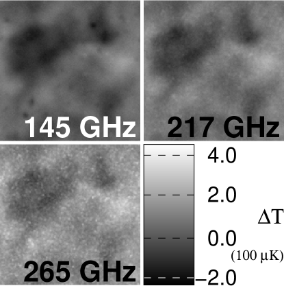
Figure 3: A simulated $1.2^{\circ}\times 1.2^{\circ}$ field in the bands of the ACT telescope. Pixel value indicates the difference in temperature from $T_{\rm CMB}$. The mean flux increases with frequency because of the increasing background of galaxies shining in the far infrared. Small scale temperature decrements at 145 GHz indicate the SZ effect.

2.8 Summary of simulations

We have constructed a 57 square degree mock CMB survey according to the specifications of ACT. It includes five astrophysical components. The CMB is a Gaussian random field, lensed by a convergence map from hydrodynamical simulations. The same simulations produced the gas pressure (for SZ) and momentum (for kSZ). Both SZ and kSZ have well defined frequency dependences. SZ is negative in the 145 GHz channel, zero in the 217 GHz channel, and positive in the 265 GHz channel. Kinetic SZ scales with frequency exactly as the primary CMB. The simulations include two types of point sources. Radio sources dim with frequency and have their greatest contribution at 145 GHz and little contribution at higher frequencies. Infrared point sources brighten with frequency, and are prominent in the 217 GHz and 265 GHz bands. We have conservatively removed the brightest radio and infrared sources. A more aggressive flux cut on radio sources can help a power spectrum analysis, if more information about the sources is available from other surveys, but we assume it is not. A more aggressive flux cut on infrared sources begins to degrade the survey area, and depending on the application may not improve the variance in a power spectrum analysis. We have to include infrared sources in any analysis because they are too numerous to excise. We include instrument noise and beam from Table 1. The instrument has highest resolution at 265 GHz and lowest at 145 GHz.

The assembled signals, convolved with the telescope beam and added to the noise, are depicted in the ACT channels in Figure 3. The striking features are the primary fluctuations on large scales, bright SZ clusters (as a decrement) at 145 GHz, and the substantial brightening of infrared point sources at higher frequencies.

The power spectra of these channels are shown in Figure 2. The power spectrum in each of the three channels is dominated by the CMB on the larger scales and instrumental noise on the smaller scales. At the intermediate scales of this survey, SZ is the most significant component in the 145 GHz band. In the bands at 217 GHz and 265 GHz, infrared point sources are the major contribution to the point sources at intermediate scales.

At this point we may draw several conclusions about these simulations. The CMB is sub-dominant on a wide range of scales accessible to this survey. The dominant cosmological features are secondary anisotropies, but these suffer from serious pollution from extragalactic point sources, particularly infrared sources in the high frequency bands. These astrophysical components exceed the noise over a wide range of interest. In section 3 we proceed with a power spectrum analysis and return to non-Gaussian features in 4.

3 Power spectrum analysis

From our simulated maps, we seek to measure the power spectra of our various cosmic signals. We use a minimum-variance quadratic estimator, which can also be viewed as an iterative procedure to find maximum-likelihood solution [25]. The power spectrum estimates are unbiased. For components that cannot be separated using the frequency information (formally in this case the Fisher matrix becomes singular and the errors infinite) it is better to treat them as a single component and then try to separate them using additional considerations such as a prior knowledge of the power spectrum shape for the signals. For some applications, power-spectrum estimators that involve the intermediate Wiener filtered maps are minimum variance [26]. However for this application, they are not necessarily minimum variance. Our approach here is a generalization of those treatments and should improve upon those estimators. As an added bonus, the effects of imperfect cleaning of one component on the mean and errors of other components are automatically included, for the estimator is unbiased and minimum variance (considering the imperfect cleaning, see [27]). For non-Gaussian signals, the estimator is unbiased, but not minimum variance. In this section, we discuss this estimator and its relation to the Wiener filter. We discuss the impact of scatter in the frequency dependence of signals. We measure the power spectra in several cases, making different assumptions about our knowledge of the point source frequency dependence. Finally, we discuss the importance of cleaning out kSZ in determining the amplitude and slope of primary fluctuations.

3.1 Multifrequency estimator

In this section we describe the power spectrum estimator we employ. We will reference a particular Fourier mode in the flat sky approximation by its wavevector $\mathbf{l}$. We use $l$ to denote the magnitude of this wavevector. We organize our data into a vector $\mathbf{e}=\{e^{\mathbf{l}}_{\alpha}\}$. The subscript $\alpha$ refers to which band the data comes from. We will reserve Greek indices to refer to the channels of the detector, $\alpha\beta\gamma$…. We say that the data is given by the sum of the response of the instrument to the signals and the noise. Dropping the mode index, we write the data in channel $\alpha$ as $e_{\alpha}$, the signal as $s_{\alpha}$, and the noise as $n_{\alpha}$. For a particular multipole, we characterize the data, signals, and noise by their covariances $\langle e_{\alpha}e_{\beta}^{*}\rangle=C_{\alpha\beta}$, $\langle s_{\alpha}s_{\beta}^{*}\rangle=S_{\alpha\beta}$ and $\langle n_{\alpha}n_{\beta}^{*}\rangle=N_{\alpha\beta}$. Note that we could additionally assume the noise between channels is uncorrelated, but it is not necessary to do so. We assume that the signal and noise are uncorrelated, and that the signal depends on a set of parameters $\mathbf{Z}=Z_{p}$. Thus, restoring the multipole dependence, the covariance matrix is

$$\mathbf{C}=\langle\mathbf{ee}^{\dagger}\rangle=C^{l}_{\alpha\beta}\delta_{\mathbf{ll}^{\prime}}$$ (9)

where

$$C^{l}_{\alpha\beta}=S^{l}_{\alpha\beta}(\mathbf{Z})+N^{l}_{\alpha\beta}.$$ (10)

The covariance matrix $\mathbf{C}$ has both frequency channel and and multipole indices, and we have assumed that different multipoles are independent, hence the $\delta_{\mathbf{ll}^{\prime}}$.

In a Gaussian model, the likelihood function for the data is

$$L(\mathbf{e})=(2\pi)^{-N/2}\det(\mathbf{C})^{-1/2}\exp(-{1\over 2}\mathbf{e}^{{\dagger}}\mathbf{C}^{-1}\mathbf{e}).$$ (11)

A second order expansion in $Z_{p}$ gives

$$\ln L(\mathbf{Z}+\delta\mathbf{Z}) = \ln L(\mathbf{Z})+\sum_{p}{\partial\ln L(\mathbf{Z})\over\partial Z_{p}}\delta Z_{p}$$ (12)

$$+{1\over 2}\sum_{pp^{\prime}}{\partial^{2}\ln L(\mathbf{Z})\over\partial Z_{p}\partial Z_{p^{\prime}}}\delta Z_{p}\delta Z_{p^{\prime}},$$

where

$$-2{\partial\ln L(\mathbf{Z})\over\partial Z_{p}} = {\rm tr\ }(\mathbf{e}^{{\dagger}}\mathbf{C}^{-1}{\partial\mathbf{C}\over\partial Z_{p}}\mathbf{C}^{-1}\mathbf{e}-\mathbf{C}^{-1}{\partial\mathbf{C}\over\partial Z_{p}})$$

$$-{\partial^{2}\ln L(\mathbf{Z})\over\partial Z_{p}\partial Z_{p^{\prime}}} = \mathbf{e}^{{\dagger}}\mathbf{C}^{-1}{\partial\mathbf{C}\over\partial Z_{p}}\mathbf{C}^{-1}{\partial\mathbf{C}\over\partial Z_{p^{\prime}}}\mathbf{C}^{-1}\mathbf{e}$$ (13)

$$-{1\over 2}{\rm tr\ }(\mathbf{C}^{-1}{\partial\mathbf{C}\over\partial Z_{p}}\mathbf{C}^{-1}{\partial\mathbf{C}\over\partial Z_{p^{\prime}}}).$$

The ensemble average of the second expression is the Fisher matrix

$$F_{pp^{\prime}}={1\over 2}{\rm tr\ }(\mathbf{C}^{-1}{\partial\mathbf{C}\over\partial Z_{p}}\mathbf{C}^{-1}{\partial\mathbf{C}\over\partial Z_{p^{\prime}}}).$$ (14)

Note that for a given value of $l$, the trace accounts for the sum over $(2l+1)f_{\rm sky}$ modes. At the maximum likelihood value the first derivative of the likelihood function vanishes, so we use the Newton-Raphson method to find the zero of the derivative. This leads to the minimum variance quadratic estimator for the parameters $\mathbf{Z}$ [28, 29, 26].

$$\hat{Z}_{p} = {1\over 2}\sum_{p^{\prime}}F^{-1}_{pp^{\prime}}[\mathbf{e}^{{\dagger}}\mathbf{C}^{-1}{\partial\mathbf{C}\over\partial Z_{p^{\prime}}}\mathbf{C}^{-1}\mathbf{e}-b_{p^{\prime}}]$$

$$b_{p} = {\rm tr\ }[\mathbf{C}^{-1}{\partial\mathbf{C}\over\partial Z_{p}}\mathbf{C}^{-1}\mathbf{N}].$$ (15)

We use $\hat{Z}_{p}$ to denote the estimate of $Z_{p}$.

In this formalism, the covariance matrix of the estimated parameters, written $\mathsf{C}_{pp^{\prime}}$, is given by the inverse Fisher matrix:

$${\mathsf{C}}_{pp^{\prime}}=\langle\hat{Z}_{p}\hat{Z}_{p^{\prime}}\rangle=F^{-1}_{pp^{\prime}}$$ (16)

This technique requires knowledge of the covariance $\mathbf{C}$. We may estimate this by taking a smoothed version of the data. If the covariance is incorrect, the estimator is still unbiased, but the error bars will be incorrect.

The parameters we desire to estimate are the power spectra of the signals, defined in a way which does not depend on the frequency channels of our instrument. We denote our signal with $\mathbf{s}=s^{\mathbf{l}}_{m}$. Here $m$ indicates which signal we are referring to. We will also use the (cross) power spectrum of signals, denoted $S^{l}_{mn}=\langle s^{\mathbf{l}}_{m}s^{\mathbf{l^{\prime}}}_{n}\rangle\delta_{\mathbf{ll}^{\prime}}$. We introduce the frequency response $\mathcal{R}_{\alpha\beta mn}$ to relate the spectra of the signals in the channels to the spectra of the signals $S^{l}_{mn}$, however we have chosen to define them. Note that $S^{l}_{mn}$ is symmetric in $m$ and $n$, so only one ordering of each pair is required. Then the cross power spectrum from the combination of channel $\alpha$ and channel $\beta$ will be given as:

$$S^{l}_{\alpha\beta}=\sum_{mn}\mathcal{R}_{\alpha\beta mn}S^{l}_{mn}.$$ (17)

We discuss the frequency response in more detail below. To estimate the power spectrum of the signals we set $Z_{p}=S^{l}_{mn}$. Note that in this case the index $p$ enumerates each combination of $lmn$. In this case the appropriate derivative of the covariance is given by

$${\partial C^{l^{\prime}}_{\alpha\beta}\over\partial Z_{p}}={\partial C^{l^{\prime}}_{\alpha\beta}\over\partial S^{l}_{mn}}=\sum_{m^{\prime}n^{\prime}}\mathcal{R}_{\alpha\beta m^{\prime}n^{\prime}}\delta_{ll^{\prime}}$$ (18)

$$\ \times\left[\delta_{mm^{\prime}}\delta_{nn^{\prime}}+\delta_{mn^{\prime}}\delta_{nm^{\prime}}-\delta_{mm^{\prime}}\delta_{nn^{\prime}}\delta_{mn^{\prime}}\delta_{nm^{\prime}}\right]$$

The final expression in the brackets is shorthand for:

$$[\dots]=\left\{\begin{array}[]{l l l}1&\parbox{108.405pt}{if ($m=m^{\prime}$ and $n=n^{\prime}$) or ($m=n^{\prime}$ and $n=m^{\prime}$),}\\ 0&\mbox{otherwise}.\end{array}\right.$$ (19)

If we know the shape of the cross spectra and wish to estimate the amplitude, we can write the signal power in the bands as

$$S^{l}_{\alpha\beta}=\sum_{mn}\mathcal{R}_{\alpha\beta mn}A_{mn}S^{l}_{mn}$$ (20)

where $A_{mn}$ encodes the information about the amplitude, and $S^{l}_{mn}$ is the shape. If we want to estimate this amplitude, then $Z_{p}=A_{mn}$. Thus the derivative of the covariance is given by

$${\partial C^{l}_{\alpha\beta}\over\partial Z_{p}}={\partial C^{l}_{\alpha\beta}\over\partial A_{mn}}=\sum_{m^{\prime}n^{\prime}}\mathcal{R}_{\alpha\beta m^{\prime}n^{\prime}}S^{l}_{mn}$$

$$\ \times\left[\delta_{mm^{\prime}}\delta_{nn^{\prime}}+\delta_{mn^{\prime}}\delta_{nm^{\prime}}-\delta_{mm^{\prime}}\delta_{nn^{\prime}}\delta_{mn^{\prime}}\delta_{nm^{\prime}}\right]$$

If we know the shape of some signals, but not others, we may use the two expressions (18) and (3.1) in combination. In these expressions we have assumed that the power spectra of the components are unknown, but that their frequency dependence is known (and hidden in $\mathcal{R}_{\alpha\beta mn}$ coefficients). If the parameters which determine the frequency scaling are not known then one can generalize this further, add these parameters to the estimate, and maximize the likelihood over them as well, provided the Fisher matrix does not become singular. The procedure of taking derivatives of the covariance matrix is similar, so we do not give such expressions here.

3.2 Relation to Wiener filter

If all signals have a spatially uniform frequency dependence, then $s^{\mathbf{l}}_{\alpha}=\sum_{m}R_{\alpha m}s^{\mathbf{l}}_{m}$ for all $\mathbf{l}$. The correlation coefficient of modes between frequency channels will be unity (neglecting noise). In this case we can factor the frequency response into a simpler form:

$$\mathcal{R}_{\alpha\beta mn}=R_{\alpha m}R_{\beta n}$$ (22)

We may put the components into a vector $\mathbf{R}_{m}=R_{\alpha m}$. This allows us to compactly express the Wiener-filtered estimates of the signal maps, which minimize the variance in reconstruction errors. The same expression holds for all modes, so we drop the mode index $\mathbf{l}$. The Wiener estimate is

$$\hat{s}_{m} = \sum_{m^{\prime}}S_{mm^{\prime}}y_{m^{\prime}}$$ (23)

$$y_{m} = \mathbf{R}_{m}^{\mathsf{T}}\mathbf{C}^{-1}\mathbf{e}.$$ (24)

The $\hat{s}_{m}$ are the Wiener filtered estimates of all signal maps. From these estimated maps of the signals, we can compute the power spectrum, taking into account the contamination from the other signals to the Wiener filtered maps. In the case of spatially uniform frequency dependence, this procedure is identical to the multifrequency estimate in the previous section. The Wiener estimate requires the power spectrum $S_{im}$, or we could use a power spectrum estimate and iterate.

For signals with non-uniform frequency dependence, it may not be possible to write a vector $\mathbf{R}_{m}$ which satisfies (22). A spatially-averaged frequency dependence may still be used to produce a Wiener-type estimate, but it is not guaranteed to be an unbiased or a minimum variance reproduction of the signal. In addition, the power spectrum obtained from these maps can be substantially biased. This is because a power spectrum estimate which uses a Wiener filtered map as an intermediate step does not account for the scatter in the frequency dependence. If this scatter is substantial, the Wiener filter may be inappropriate. (See [30] for making minimum variance maps of signals with good frequency coherence in the presence of incoherent foregrounds. To make a map of an incoherent signal, like a point source template, this approach may not be minimum variance. See [27] for a generic model of frequency incoherence.)

3.3 Frequency dependence and scatter

To apply the multifrequency filter, one needs the noise power spectra and signal frequency dependences. We assume the noise power spectrum in the three channels is well known. The frequency scalings of CMB and kSZ signals are constant in temperature units, so the relevant components of $\mathcal{R}_{\alpha\beta mn}$ are unity. For SZ, the frequency dependence is from equation 3. The frequency dependence of point sources are poorly known. Significant modeling or outside observations are needed to fill in the remaining components of $\mathcal{R}_{\alpha\beta mn}$. These cannot be completely determined from ACT alone in an unbiased way. If they are added to the parameter vector $Z_{p}$ without any additional assumptions, the Fisher matrix becomes singular. This means these parameters are completely degenerate with the power spectra: there exists a family of power spectra and frequency dependences which reproduces the covariance, and it is impossible to distinguish between individual members of this family.

It is possible, however, that for given models of the point source emission, the parameters of the model may be added to the estimate without forcing the Fisher matrix to be singular. Additionally, we can use the high $l$ part of the spectrum, which is dominated by point source emission, to help constraint frequency dependence, at the expense of biasing our estimator. We use this in the following section.

In our simulations, the frequency scaling differs substantially from point source to point source. The correlation coefficient between modes at different frequencies is less than unity, so the cross spectrum is less than predicted from the auto-powers. It may be senseless to produce a Wiener filtered signal estimate based on a spatially averaged frequency dependence. We do not use a spatially averaged frequency dependence in our power spectrum estimations, for we find it produces greater than $2\sigma$ biases in the power measurement. The conclusion is that it is crucial to address the scatter in the frequency dependence of point sources.

ACT and similar experiments will identify a population of bright sources, which may be used to study their frequency scaling. One should apply this information to a power spectrum analysis with some caution, because the sources which contaminate the power spectrum analysis are dimmer than the population which is convenient to study. This may mean that contaminating sources are a different population, more distant, younger and less evolved, or some combination. Dust emission is complicated, and the emission spectra of the point sources likely depends on the relative abundances of the dust species present. If the populations are different, it will be difficult to build an accurate model of the emission from these sources. In addition, bright sources may result from the confusion of two dimmer sources. Measurements of the scatter of source frequency dependence is then difficult to interpret.

High-resolution interferometric measurements would help in studying the source population. In particular, ALMA has frequency coverage in the ACT bands. It should have sufficient sensitivity to pick out sources which are confusing ACT, and sufficient angular resolution to resolve them. As mentioned, masking infrared sources to a low flux cut is not very promising, but ALMA would be useful as a tool to explore the frequency dependence and scatter of sources.

3.4 Measured signal power spectrum

We measure the power spectrum in several cases assuming differing prior knowledge. Our list of cases is not exhaustive, but illustrates techniques one might explore. We always assume the frequency dependence of CMB, kSZ, and SZ. We enumerate our assumptions, and the parameters to estimate in each case.

The first two cases assume we have perfect knowledge of the point source frequency scaling and scatter.

Case 1. We assume we know the frequency dependence of the point sources. The parameters to estimate are the power spectra, in bins, of CMB$+$kSZ, SZ, IR and radio point sources.

Case 2. We assume we know the power spectrum shape and frequency dependence of the point sources. The parameters to estimate are the binned power spectra of CMB$+$kSZ and SZ, and 2 amplitudes, for the IR and radio power spectra.

The next two cases assume nothing about the point source frequency dependence.

Case 3. We assume we know the shape of the point sources, and that the CMB$+$kSZ makes no contribution at $l>15000$. The final condition ensures a non-singular Fisher matrix. We treat the point sources as a single population. Parameters to estimate are the binned power spectra of CMB$+$kSZ and SZ, and 6 amplitudes, corresponding to the point source amplitude in the cross-correlations between the bands. This is equivalent to estimating the frequency dependence of the sources.

Case 4. Like case 3, but without assuming the shape of the point source power spectrum. We treat point sources as a single population, assuming that the scatter in the frequency dependence is constant as a function of scale, but we do not assume what it is. Parameters to estimate are the binned power spectra of CMB$+$kSZ and SZ, the 3 binned auto-power spectra of point sources in the three bands, and 3 correlation coefficients, which describe the scatter in the frequency relation.

The final two cases separate kSZ from the CMB using a template for the kSZ power spectrum.

Case 5. Like case 2, including point source frequency and power spectrum shape information, but with two more assumptions. First, we assume the shape of kSZ power spectrum. Second, we assume the CMB makes negligible contributions to the power for $l>6000$. The second additional assumption prevents a singular Fisher matrix. The parameters to estimate are the binned power spectra of CMB and SZ, and 3 amplitudes, for the kSZ, IR, and radio power spectra.

Case 6. Like case 3, including only point source power spectrum shape information, but with the additional assumptions of case 5. Parameters to estimate are the binned power spectra of CMB$+$kSZ and SZ, 6 point source amplitudes, and the amplitude of the kSZ spectrum.

If the parameters we choose to estimate can faithfully represent the real world, our estimate is unbiased. However, in any of our cases, an incorrect assumption can bias the estimate. Note that case 4 requires the least outside information.

Where we use a frequency dependence, we use 265 GHz as our reference frequency for SZ and infrared sources, and 145 GHz for radio sources. This choice is a convention, and has no bearing on the quality of the estimate.

We estimate the covariance on the measured power spectra in two ways. First we use the inverse Fisher matrix, so the error on the estimate of power bin $p$ is $(F_{pp}^{-1})^{1/2}$. Second, we computed the covariance from the estimates on our 40 realizations. In Figure 4, we show the errors on these power estimates as a function of $l$. In the regime where instrumental noise dominates (at sufficiently high $l$), the inverse Fisher matrix provides a good estimate of the errors. Elsewhere, we find the inverse Fisher matrix underestimates the error, due to the non-Gaussianities. Experiments of this type will likely need to rely on Monte Carlo simulations for their errors.

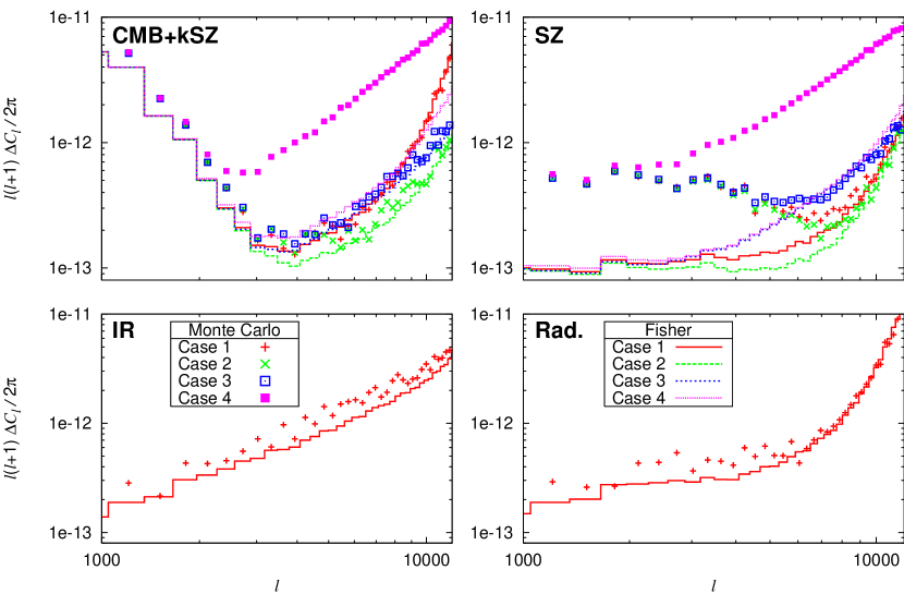
Figure 4: The errors on the estimated power spectrum. Lines indicate errors derived from the Fisher matrix: $(F_{pp}^{-1})^{1/2}$. Symbols indicate the measured standard deviation from 40 realizations. The errors in case 5 are similar to case 2, and the errors in case 6 are similar to case 3. The bottom panels show only case 1. For cases which assume the shape of the point source power spectrum, plotting the errors as a function of $l$ is not possible.

We now discuss each case in turn. The assumption in case 1 and 2 of point source frequency knowledge is probably dangerous if we do not have such knowledge. A poor model will bias the power spectrum in a way which may be hard to predict. On the other hand, if we do have a good understanding of the source population (from ALMA perhaps), cases 1 and 2 represent ideal situations. For case 1, the measured power spectrum is shown in Figure 5. In this plot we use the errors evaluated over our independent realizations. Except for radio sources, we recover the power spectra well. This provides information about the shape of the power spectrum, which we have not assumed. Our result in case 1 is unbiased.

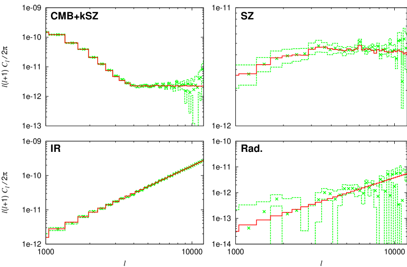
Figure 5: Estimates of the power spectra in case 1, where we assume frequency information, but no information about the shape of any power spectrum. The solid line is the true value of the power spectrum. The $\times$ symbols show the estimated value of the power spectrum. The dashed lines show 1 standard deviation above and below the estimate, evaluated over our 40 realizations. This estimate is unbiased. The width of the bins is $\Delta l\approx 300$.

We compared the inverse Fisher matrix and the covariance matrix from the realizations. In case 1, the inverse Fisher matrix is diagonal in $l$. However, we find that the actual covariance matrix is not. The covariance between the CMB+kSZ power bins is nearly diagonal in this case, but to $l$ of a few thousand, the SZ power bins are strongly correlated.

For case 2, assuming the shape of the point source power spectrum improved the errors on the CMB+kSZ power spectrum by a factor of $\sim 4$ relative to case 1. The errors on SZ are marginally improved. The power spectrum bins are somewhat correlated. In case 2, the error in the power spectrum amplitude in IR and radio point sources is $\Delta C_{l}/C_{l}=5.0\times 10^{-3}$ and $\Delta C_{l}/C_{l}=0.20$ respectively. Recall that this case combines all the information on the point source spectra into two amplitudes. The inverse Fisher matrix underestimates this error by a factor of 2. We do not plot case 2 because it is unbiased and similar to case 1, with smaller error bars, although the bins are more correlated.

Case 3 does not depend on prior frequency information, but has its own problems. Case 3 depends on an incorrect assumption that only point sources contribute at high $l$, while kSZ continues to have some small contribution at these $l$. Thus the power spectrum we deduce for point sources is slightly high, and this biases our measurement somewhat. This is relatively independent of the $l$ cutoff. We plot the measured power spectrum in Figure 6, where the bias is apparent. The power spectrum bins are also somewhat correlated. However, we needed no model for the point source frequency dependence. Our model is biased by as much as 1$\sigma$ at high $l$, but the bias is probably under better control than it would be for a model of frequency dependence, because at least we know in which direction our estimate is biased.

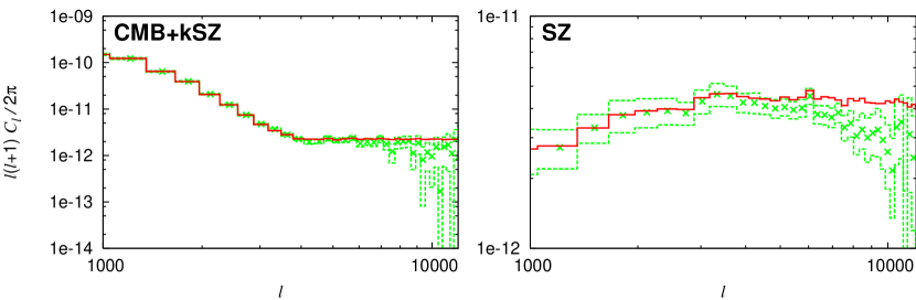
Figure 6: Estimates of the power spectra in case 3, where we assume the shape of the point source power spectrum, but assume nothing about frequency dependence.

Case 4 assumes less about the point sources than case 3, because it does not assume a shape for the power spectrum. We plot the power spectrum of CMB+kSZ and SZ in Figure 7. This case does not successfully recover kSZ. There is a systematic bias in the SZ, but statistical errors dominate. The bins are strongly correlated. Systematic biases dominate statistical errors in the recovery of the point source power spectrum. The relative bias is greatest at 145 GHz, where the point source contribution is the least, and decreases at higher frequencies. Note that in case 4 especially, the Fisher matrix characterizes the errors poorly.

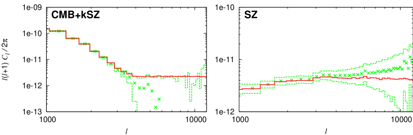
Figure 7: Estimates for case 4. Assuming no information about the power spectrum shape or frequency dependence of the point sources, we lose the ability to reliably detect kSZ. The estimate for SZ is biased, but the statistical errors are large. The bins are highly correlated.

In cases 5 and 6, the kSZ is separated from the CMB. This is necessary to allow parameter estimation based on the CMB. Because the CMB and kSZ are degenerate in frequency, this requires a model for the kSZ power spectrum. The estimator in this case uses the high $l$ portion of the kSZ spectrum, where CMB is not significant, to calibrate the model of kSZ. kSZ is then subtracted at low $l$. We use a 1-parameter model for the kSZ power spectrum where the shape is known but the amplitude is not. The approach generalizes to a multiparameter model. We do not plot case 5. For case 6, we plot the recovered power spectrum (Figure 8). We do not detect a bias on the CMB in either case, although the SZ power spectrum is biased in case 6 as it was in case 3. The CMB power bins for $l>3000$ are correlated by the kSZ template subtraction. SZ bins are also strongly correlated.

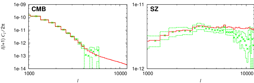
Figure 8: Estimates of the power spectra in case 6, where we assume the shape of the kSZ and point source power spectra, but assume nothing about the point source frequency dependence.

We now summarize our power spectrum analysis results. Given a good understanding of the frequency dependence of point sources, we may successfully estimate the power spectrum of each component, provided we treat the CMB and kSZ as a single component. With no prior knowledge of the frequency dependence of point sources, we may make a somewhat biased estimate of the power spectra if we know the shape of the point source power spectrum. Knowing neither the frequency dependence nor the shape of sources, we detect SZ, but cannot positively identify kSZ. For us to have confidence in our estimates, we must trust our knowledge of the point source frequency dependence. This prospect is unclear. If we do not have confidence in our frequency knowledge, we may still make an estimate of the power spectrum, but it will be somewhat biased. In our more optimistic cases, if we want to estimate CMB without kSZ, we require a parameterized model for kSZ. The power spectrum template will likely come from simulation. However, any parameterized fit to the power spectrum of the signal components may introduce a bias.

3.5 Measuring primordial amplitude and slope

In our model, the kSZ power is already comparable to the size of the CMB error bars at $l\sim 2000$, so if we do not know the kSZ power spectrum at all then we should not use the CMB power spectrum beyond there. With a model for the kSZ power spectrum we may use bins with higher $l$, as in our cases 5 and 6. To illustrate this difference, we compute the covariance matrix for primordial amplitude $A$ and slope $n$ about the fiducial values $A=1$ (COBE normalized) and $n=1$. To convert from errors on binned power to errors on parameters we use

$${\sf C}^{-1}_{qq^{\prime}}=\sum_{ll^{\prime}}\frac{dC_{l}}{dq}{\sf C}^{-1}_{ll^{\prime}}\frac{dC_{l}}{dq^{\prime}}$$ (25)

where ${\sf C}_{qq^{\prime}}$ is the covariance matrix for parameters $q$, ${\sf C}_{ll^{\prime}}$ is the covariance matrix for the binned power, consisting of the covariances computed for CMB. For this we use the CMB block of the covariance matrix for case 6. (The result using case 5 is similar.) We compute the derivatives of the power spectrum using CMBFAST. Then for primordial amplitude and slope, we have the following covariance matrix if we do not extract kSZ.

$${\bf\sf C}(l<2000)=\left\{\begin{array}[]{c|cc}&A&n\\ \hline\cr A&2\times 10^{-2}&-4\times 10^{-3}\\ n&&1\times 10^{-3}\\ \end{array}\right\}.$$ (26)

However, if we can extract the CMB, the covariance improves.

$${\bf\sf C}=\left\{\begin{array}[]{c|cc}&A&n\\ \hline\cr A&4\times 10^{-3}&-9\times 10^{-4}\\ n&&2\times 10^{-4}\\ \end{array}\right\}.$$ (27)

Thus the covariance increases by roughly a factor of 5 for $A$ and $n$ if the kSZ is not extracted. If inhomogeneous reionization raises the kSZ power, shortening further the lever arm of the CMB, it becomes more important to extract kSZ.

To gain this additional information from the CMB on scales $l>2000$ we need a template for kSZ. This template will come from simulations, and may be calibrated on the kSZ measured at higher $l$. However, there will be uncertainties in the template because of missing physics, such as patchy reionization. Therefore the power spectrum analysis should be checked in as many ways as possible against the data. One way we explore in the next section is using the non-Gaussian information.

4 One-point distribution function analysis

CMB and kSZ cannot be distinguished in a multifrequency analysis. We have seen this in our power spectrum analysis in the previous section, in which we could only estimate CMB separately from kSZ by knowing the shape of the kSZ power spectrum beforehand. However, if the data do not represent a Gaussian random field, and our data do not, then the power spectrum does not extract all the information available.

Statistics which highlight non-Gaussianity are also particularly interesting because in the standard picture, primary CMB fluctuations are Gaussian. Any non-Gaussianities indicate deviations from the standard picture for primary fluctuations, or in our case, indicate the presence of secondary sources of anisotropy.

In principle then, it is possible to use non-Gaussianities to tease apart the CMB and kSZ. In the following, we show this is possible, and explore one method for doing so. The statistic we choose is the histogram of pixel temperatures, that is, the 1-point probability distribution function (pdf). In the context of weak lensing, the pdf provides stronger constraints than simple statistics such as skewness [31]. This makes sense because the pdf incorporates all the moments of the field evaluated at a single point, such as variance, kurtosis, and so on. For a Gaussian field the pdf is Gaussian. For a highly non-Gaussian field, such as kSZ, the pdf function may show strong tails. The information in the pdf is complementary to the information in the power spectrum. The pdf contains information about non-Gaussianities, but not about spatial correlations, because it is evaluated at a single point. The power spectrum contains information about spatial correlations, but not about non-Gaussianities.

Below, we devise a method for examining the pdf of our maps to extract parameters of the component signals, given a set of templates. Then we apply this method. We want to separate CMB from kSZ, so we consider the sky at 217 GHz. This is simplest because it eliminates the signal from thermal SZ. We want to focus on scales where neither the CMB nor kSZ completely dominates the other. Thus, before evaluating the pdf, we spatially filter the maps. In Fourier space, we multiply the maps by a Gaussian centered at $l\approx 3600$ with standard deviation $\sigma_{l}\approx 750$. In figure 9, this filter is shown with the the power spectra of the various components of the sky at 217 GHz.

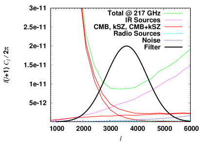
Figure 9: The spatial filter used for the non-Gaussian analysis and the components at 217 GHz. The vertical scale of the filter in this plot is arbitrary.

In the next sections, we describe the pdfs of the major signals at 217 GHz in this window, describe our method for separating kSZ from CMB, and apply it to our simulated maps.

We make no claim that this is an optimum method for separating CMB and kSZ. At this point, this method is intended as a demonstration of the power of using simple statistics which are sensitive to non-Gaussianities.

4.1 Signal one-point distribution functions

Here we examine the pdfs of the signals with the goal of identifying features that distinguish CMB and kSZ. In addition, the infrared sources will be an unavoidable contaminant at 217 GHz. The radio sources are not very significant, and as we have mentioned, may be helped by additional masking. The noise after spatial filtering is very low. After spatial filtering, we show the histograms for the major signals at 217 GHz in Figure 10.

The pdf of the unlensed CMB is Gaussian. After lensing, the distribution is still Gaussian because lensing simply remaps locations on the sky. After spatial filtering, the lensed CMB need not have a Gaussian distribution function, but we find the deviations in this case to be insignificant.

The distribution of kSZ should be symmetric, because there should be roughly as many clusters moving towards us as away. We expect the pdf of kSZ, or any signal sourced by discrete objects, to have a non-Gaussian point distribution function. This is because the signal strength is highly localized: the values of pixels are extreme in the direction of the object, and zero elsewhere. The kSZ histogram shows tails well beyond that expected from a Gaussian pdf of the same variance. A pdf with power law tails, such as Student’s $t$-distribution, is a much better fit, although we find the $t$-distribution to be too poor of a model to apply our method.

We might expect the point sources to have a non-Gaussian pdf, since they are positive definite, which would seem to argue for strong skewness. This is counteracted by two effects. For a high density of sources, several sources are included in each beam, and the non-Gaussianity is diminished due to central limit theorem considerations. In addition, our spatial filtering removes long wavelength modes, causing ringing about each source which can wash out skewness. We show the histogram for infrared point sources, after spatial filtering, in figure 10; it is nearly Gaussian. A wider window function reduces ringing, and produces a point source pdf which is more positively skewed.

We see that the tails of the kSZ distribution are a unique feature with which we can try to distinguish it from the other signals.

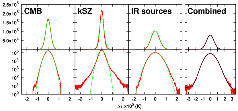
Figure 10: The histograms of the major signals at 217 GHz, after spatial filtering. Each pair of plots shows the same data, except the vertical axis above has a linear scale and below has a log scale. The distributions have been normalized to unity. The CMB is well fit by a Gaussian. kSZ is poorly fit by a Gaussian with the same variance. Infrared point sources are slightly skewed in the positive direction, compared to a Gaussian. At right we show the histogram of the sum of these maps, along with our best fit pdf from fitting and convolving the template pdfs, as described in the text.

4.2 Likelihood

Given a set of pixelized data, we want to examine the likelihood of a trial distribution function. Let $P_{\mathbf{a}}(\Delta T)$ be a trial pdf, which depends on a set of parameters $\mathbf{a}$. For now, think of it as an abstract parameterized model for our data histogram. We construct our trial pdf in the next section. For a set of independent pixels $\Delta T_{i}$, the likelihood of parameters $\mathbf{a}$ is given by

$$L(\mathbf{a})=\prod_{i}P_{\mathbf{a}}(\Delta T_{i}),$$ (28)

which is just the probability of the first pixel, times that of the second, and so on. Computationally it is more convenient to work with the logarithm of the likelihood. We also work with a binned pdf, so we combine all the pixels for each bin, and sum over bins:

$$\log L(\mathbf{a})=\sum_{j}N_{j}\log P_{\mathbf{a}}(\Delta T_{j}),$$ (29)

where $N_{j}$ is the number of pixels in histogram bin $j$, and $\Delta T_{j}$ is the value at the center of bin $j$. This gives us the likelihood of parameters $\mathbf{a}$ for model pdf $P_{\mathbf{a}}(\Delta T)$ in terms of the histogram of pixel values $N_{j}$.

If the pixels are not all independent, this is not the correct likelihood function. The true likelihood would take into account the covariance between pixels (or alternatively, between bins). However, we find in practice that the peak of the given likelihood function in (29) is a good enough estimate for this application. The correlation length of our maps after spatial filtering is much less than the size of the maps. Thus our maps contain a large number of uncorrelated patches. If these patches are thought of as larger, independent pixels, then the likelihood we have written has the right peak, but may have a wrong normalization and width. In our method, we use only the location of the likelihood peak, while the errors are assessed using Monte Carlo simulations.

Our goal is to find the set of parameters $\mathbf{a}$ which maximize the likelihood. We use Powell’s direction set method [32]. Because the data (the histogram of pixel temperatures) is noisy, the likelihood function is plagued by local maxima. We repeat our maximum likelihood search with randomized initial positions and search directions in parameter space, to ensure that the maximum we find is reliable.

We compute errors on our parameters by the bootstrap method. We sample our sky map realizations (with replacement) to generate synthetic data histograms. We find the maximum likelihood parameters for each of these synthetic histograms, and use the distribution of these to describe the probability distribution for the parameters.

4.3 Separation by distribution function

To evaluated the likelihood function (29), we need a parameterized model pdf for the data histogram at 217 GHz. To get unbiased estimates of the parameters, our model must faithfully reproduce the data. We proceed by making models of each signal in turn. The pdf of the sum of independent random variables is given by the convolution of the pdfs of the individual random variables. Therefore, by modeling the pdfs of the individual signals, we can produce a trial pdf for the total data by convolution. We use binned functions for our models, and evaluate the convolution with fast Fourier transforms. Our procedure is not very sensitive to the width of the bins unless the model pdfs contain sharp features. In this application, our pdfs are smooth functions, and we find that roughly one thousand bins covering the pdf suffices.

We make a 2 parameter model for the pdf. Our parameters are the quantities we seek to estimate, in this case the standard deviation of the CMB, which we label $\sigma_{\textrm{\scriptsize CMB}}$, and the standard deviation of the kSZ, which we label $\sigma_{\textrm{\scriptsize kSZ}}$. For the model pdf of the CMB we simply use a Gaussian with variance $\sigma_{\textrm{\scriptsize CMB}}^{2}$. For the kSZ pdf, we use the actual histogram of the kSZ as a template. In the real experiment, this would not be available, but could be based on simulations. To generate a distribution with a given standard deviation we rescale the template, preserving the distribution’s unit integral. For the model pdf of the point sources, we again use the actual point source histogram as a template. If we understand the point source population well enough to make a good power spectrum analysis, such that we wish to attempt a separation of CMB and kSZ, the we should be able to model the point source pdf. Note that our non-Gaussian analysis will provide a constraint on $\sigma_{\textrm{\scriptsize CMB}}$ and $\sigma_{\textrm{\scriptsize kSZ}}$ individually. Contrast this to the power spectrum analysis, which constrains only the total variance $\sigma_{\textrm{\scriptsize CMB}}^{2}+\sigma_{\rm kSZ}^{2}$, albeit in a narrower window of multipoles.

We apply our maximum likelihood parameter estimate to this model. The result is a $>10\sigma$ detection of the CMB and a $>7\sigma$ detection of the kSZ in our window (see Figure 11). The estimate is somewhat degenerate in the direction which preserves the total variance $\sigma_{\textrm{\scriptsize CMB}}^{2}+\sigma_{\rm kSZ}^{2}$.

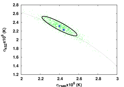
Figure 11: Separating CMB from kSZ using the pdf. This plot shows the result of our fitting procedure for the standard deviation of the kSZ and CMB. The “$+$” shows the best fit point. The “$\times$” marks the true value. The dots show the distribution of the fits for 1000 bootstrap realizations. The contour denotes the 68% region computed from the covariance of the bootstrap points ($\chi^{2}$ with 2 degrees of freedom). The fine dotted line shows the circle of constant total variance which passes through the true value.

The power of this method arises from the template for kSZ, which fixes the relation between the kSZ pdf’s variance and tails. If this relationship is not fixed, then a narrow kSZ distribution with wide tails could mimic a wide kSZ distribution with narrow tails, by adjusting the variance of the CMB pdf to compensate. Also, it is crucial to have the point source contribution constrained. Otherwise it would be degenerate with the CMB.

We must depend on simulations for the relationship between the variance and tails of kSZ. This non-Gaussian method may also be viewed as a consistency check for kSZ template simulations. A simulation of kSZ must both satisfy the power spectrum at high $l$, and provide the correct non-Gaussianity where kSZ and CMB overlap. If the measurements differ, one should not have confidence in the template power spectrum for kSZ provided by the simulation.

5 Conclusions

We have developed simulations of the ACT experiment in three frequency bands and analyzed the ability of ACT to extract the power spectrum and non-Gaussian statistics from it. The simulations include CMB, kSZ, SZ, and radio and infrared point sources. Secondary anisotropies dominate the CMB over a wide range of interest. These in turn are heavily polluted by point sources. Infrared point sources must be dealt with in the power spectrum, and cannot be completely dealt with by masking. While we included the latest constraints on the secondary anisotropies, significant uncertainties on the amplitude and correlation properties remain and could affect the conclusions reached in this paper. Particularly uncertain is the contribution of patchy reionization to kSZ.

An optimal multifrequency filter can extract the power spectrum, but the results are subject to assumptions put into the analysis. We considered several cases, making different assumptions about our knowledge of contaminating extragalactic point sources. For optimal extraction knowing both the mean and scatter of the frequency dependence of point sources is crucial. If we do not use a prior model for the frequency dependence of the point sources we may still extract the power spectrum assuming spatial correlations are known, but the results may still be biased. Furthermore, using only frequency information in a power spectrum analysis, kSZ and CMB cannot be separated using data alone. This degrades the ability to measure the CMB at $l>2000$ and to determine parameters from it.

We also explored the ability to use the non-Gaussian information to constrain further the individual components. Non-Gaussianities in the histogram of pixel temperatures at 217 GHz should be observable by ACT. Non-Gaussianities created by kSZ can allow one to distinguish it from Gaussian CMB on scales where the two cannot be separated with the power spectrum analysis, assuming that simulations are able to provide an accurate template of kSZ. It is unclear how well a kSZ template from simulations will work when applied to, for example, kSZ created by patchy reionization. Therefore, our results are preliminary and more investigation of these techniques is needed. Combining the power spectrum template analysis with the non-Gaussian template analysis allows one to perform consistency checks among these methods.

Our results suggest that extracting the primordial power spectrum information at high precision from small scale primary CMB will be challenging. Scatter in the frequency scaling of point sources, as well as their possible correlations, make the point source separation from CMB difficult. Assuming this is accomplished, removing kSZ is even more difficult and can only be done with reliable templates for the power spectrum and for non-Gaussian signals. The final precision is likely to be limited by the modeling uncertainties and not by the statistical precision of the observations. It is hard to prognosticate the final accuracy given how uncertain the kSZ amplitude from patchy reionization is. In this context it is worth mentioning that CMB polarization has fewer secondary anisotropies to worry about than the CMB temperature anisotropy itself and so may ultimately be more promising as a tool to study the primordial power spectrum fluctuations on small scales.

References

- [1] A. Kosowsky. The Atacama Cosmology Telescope. New Astronomy Review, 47:939–943, December 2003.
- [2] P. Zhang, U. Pen, and B. Wang. The Sunyaev-Zeldovich Effect: Simulations and Observations. ApJ, 577:555–568, October 2002.
- [3] U. Pen. A high-resolution adaptive moving mesh hydrodynamic algorithm. ApJS, 115:19+, March 1998.
- [4] U. Seljak, J. Burwell, and U. Pen. Sunyaev-Zeldovich effect from hydrodynamical simulations: Maps and low order statistics. Phys. Rev. D, 63:63001–+, March 2001.
- [5] P. Zhang, U. Pen, and H. Trac. Precision era of the kinetic Sunyaev-Zeldovich effect: simulations, analytical models and observations and the power to constrain reionization. ArXiv Astrophysics e-prints, pages 4534–+, April 2003.
- [6] U. Seljak and M. Zaldarriaga. A line-of-sight integration approach to cosmic microwave background anisotropies. ApJ, 469:437+, October 1996.
- [7] M. Zaldarriaga and U. Seljak. Reconstructing projected matter density power spectrum from cosmic microwave background. Phys. Rev. D, 59:123507–+, June 1999.
- [8] C. M. Hirata and U. Seljak. Analyzing weak lensing of the cosmic microwave background using the likelihood function. Phys. Rev. D, 67:43001–+, February 2003.
- [9] M. Birkinshaw. The sunyaev-zel’dovich effect. Phys. Rep., 310:97–195, March 1999.
- [10] J. E. Carlstrom, G. P. Holder, and E. D. Reese. Cosmology with the Sunyaev-Zel’dovich Effect. ARA&A, 40:643–680, 2002.
- [11] A. C. da Silva, D. Barbosa, A. R. Liddle, and P. A. Thomas. Hydrodynamical simulations of the Sunyaev-Zel’dovich effect. MNRAS, 317:37–44, September 2000.
- [12] V. Springel, M. White, and L. Hernquist. Hydrodynamic simulations of the sunyaev-zeldovich effect(s). ApJ, 549:681–687, March 2001.
- [13] M. White, L. Hernquist, and V. Springel. Simulating the Sunyaev-Zeldovich Effect(s): Including Radiative Cooling and Energy Injection by Galactic Winds. ApJ, 579:16–22, November 2002.
- [14] A. Refregier and R. Teyssier. Numerical and analytical predictions for the large-scale Sunyaev-Zel’dovich effect. Phys. Rev. D, 66(4):043002–+, August 2002.
- [15] E. Komatsu and U. Seljak. The Sunyaev-Zel’dovich angular power spectrum as a probe of cosmological parameters. MNRAS, 336:1256–1270, November 2002.
- [16] A. Cooray. Large scale pressure fluctuations and the Sunyaev-Zel’dovich effect. Phys. Rev. D, 62:103506+, 2000.
- [17] P. Zhang, U. Pen, and H. Trac. Precision era of the kinetic Sunyaev-Zel’dovich effect: simulations, analytical models and observations and the power to constrain reionization. MNRAS, 347:1224–1233, February 2004.
- [18] A. C. da Silva, D. Barbosa, A. R. Liddle, and P. A. Thomas. Hydrodynamical simulations of the Sunyaev-Zel’dovich effect: the kinetic effect. MNRAS, 326:155–163, September 2001.
- [19] M. G. Santos, A. Cooray, Z. Haiman, L. Knox, and C. . Ma. Small-scale CMB Temperature and Polarization Anisotropies due to Patchy Reionization. May 2003.
- [20] G. De Zotti, F. Perrotta, G. L. Granato, L. Silva, R. Ricci, C. Baccigalupi, L. Danese, and L. Toffolatti. Millimeter-band Surveys of Extragalactic Sources. ArXiv Astrophysics e-prints, pages 4038–+, April 2002.
- [21] L. Toffolatti, F. Argueso Gomez, G. de Zotti, P. Mazzei, A. Franceschini, L. Danese, and C. Burigana. Extragalactic source counts and contributions to the anisotropies of the cosmic microwave background: predictions for the Planck Surveyor mission. MNRAS, 297:117–127, June 1998.
- [22] T. Totani and T. T. Takeuchi. A Bridge from Optical to Infrared Galaxies: Explaining Local Properties and Predicting Galaxy Counts and the Cosmic Background Radiation. ApJ, 570:470–491, May 2002.
- [23] J. Miralda-Escudé, M. Haehnelt, and M. J. Rees. Reionization of the Inhomogeneous Universe. ApJ, 530:1–16, February 2000.
- [24] Y. Song, A. Cooray, L. Knox, and M. Zaldarriaga. The Far-Infrared Background Correlation with Cosmic Microwave Background Lensing. ApJ, 590:664–672, June 2003.
- [25] J. R. Bond, A. H. Jaffe, and L. Knox. Estimating the power spectrum of the cosmic microwave background. Phys. Rev. D, 57:2117–2137, February 1998.
- [26] U. Seljak. Cosmography and Power Spectrum Estimation: A Unified Approach. ApJ, 503:492–+, August 1998.
- [27] M. Tegmark, D.J̃. Eisenstein, W. Hu, and A. de Oliveira-Costa. Foregrounds and forecasts for the cosmic microwave background. ApJ, 530:133–165, February 2000.
- [28] A. J. S. Hamilton. Towards optimal measurement of power spectra - I. Minimum variance pair weighting and the Fisher matrix. MNRAS, 289:285–294, August 1997.
- [29] M. Tegmark. How to measure CMB power spectra without losing information. Phys. Rev. D, 55:5895–5907, May 1997.
- [30] A. Cooray, W. Hu, and M. Tegmark. Large-Scale Sunyaev-Zeldovich Effect: Measuring Statistical Properties with Multifrequency Maps. ApJ, 540:1–13, September 2000.
- [31] B. Jain, U. Seljak, and S. White. Ray-tracing simulations of weak lensing by large-scale structure. ApJ, 530:547–577, February 2000.
- [32] W. H. Press, B. P. Flannery, and S. A. Teukolsky. Numerical recipes. The art of scientific computing. Cambridge: University Press, 1986, 1986.