Gravitational lensing of the CMB by galaxy clusters

We adapt a non-linear filter proposed by Hu (2001) for detecting lensing of the CMB by large-scale structures to recover surface-density profiles of galaxy clusters from their localised, weak gravitational lensing effect on CMB fields. Shifting the band-pass of the filter to smaller scales, and normalising it such as to reproduce the convergence rather than the deflection angle, we find that the mean density profile of a sample of 100 clusters can be recovered to better than 10% from well within the scale radius to almost the virial radius. The kinetic Sunyaev-Zel’dovich effect is shown to be a negligible source of error. We test the filter applying it to data simulated using the characteristics of the Atacama Cosmology Telescope (ACT), showing that it will be possible to recover mean cluster profiles outside a radius of $1^{\prime}$ corresponding to ACT’s angular resolution.

1 Introduction

Future observations of large fractions of the sky in the sub-mm regime are expected to detect of order $10^{4}$ galaxy clusters through their thermal Sunyaev-Zel’dovich (tSZ) effect (da Silva et al., 2000; Bartelmann, 2001; Carlstrom et al., 2002). They appear projected on the CMB, which is relatively feature-less on the angular scales typical for galaxy clusters. The weak gravitational lensing caused by the clusters will distort the CMB pattern in a characteristic way (Seljak & Zaldarriaga, 2000). It appears unlikely that the lensing signal of individual clusters on the CMB will be detectable with current experiments, but it may be possible to extract statistical information on the cluster mass distribution by suitably combining the signal caused by large cluster subsamples. Future instruments like ALMA with high sensitivity and resolution should even be able to detect lensing by few or single clusters.

Various possibilities for detecting cluster lensing signals in the CMB were recently discussed. Holder & Kosowsky (2004) suggested to use Wiener filtering for estimating the unlensed temperature map, which is then subtracted from the measured lensed map to obtain the deflection field. Vale et al. (2004) proposed a conceptually similar technique based on subtracting an estimate of the unlensed CMB background, obtained by fitting a temperature gradient to the observed map.

We follow a different route, starting from a non-linear filter suggested by Hu (2001) for extracting the lensing signal of large-scale structure from CMB observations. Since the CMB on cluster scales can be locally approximated by a gradient, the cluster-lensed CMB temperature pattern is randomly oriented. Aiming at a technique which allows cluster-sized CMB images to be stacked in order to extract statistical information on cluster profiles, we thus require a filter which is non-linear in the signal. Hu’s filter essentially measures the squared gradient of the temperature map and thereby renders the filtered maps suitable for stacking. We modify the filter in two ways which turn out to improve it substantially when applied to lensing by clusters rather than large-scale structures.

The plan of the paper is as follows: We summarise CMB lensing and introduce the filter in Sect. 2. In Sect. 3, we describe simulations of clusters and cluster samples. In Sect. 4, we apply the filter to these simulations, taking the kinetic Sunyaev-Zel’dovich (kSZ) effect and instrumental noise into account. We summarise and discuss our results in Sect. 5.

2 Lensing of the CMB and filtering

Lensing by a thin mass distribution on a single plane can be described by the scalar lensing potential

$$\psi(\@vec{\theta})=\frac{2}{c^{2}}\frac{D_{\mathrm{ds}}}{D_{\mathrm{d}}D_{\mathrm{s}}}\int\Phi(D_{\mathrm{d}}\@vec{\theta},z)\mathrm{d}z\;,$$ (1)

where $D_{\mathrm{d,s,ds}}$ are the angular-diameter distances from the observer to the lens, the source, and from the lens to the source, respectively, and $\Phi$ is the Newtonian gravitational potential of the lensing mass distribution, which is integrated along the line-of-sight. The deflection angle $\@vec{\alpha}=\@vec{\nabla}\psi$, and the convergence $\kappa=\@vec{\nabla}^{2}\psi/2$ is the scaled surface-mass density (see e.g.  Schneider et al., 1992; Narayan & Bartelmann, 1999, for reviews).

Light rays propagating into a direction $\@vec{\theta}$ on the sky are deflected by the angle $\@vec{\alpha}(\@vec{\theta})$. Thus, the CMB temperature $T(\@vec{\theta})$ observed into direction $\@vec{\theta}$ is the intrinsic temperature $\tilde{T}$ at a slightly shifted position,

$$T(\@vec{\theta})=\tilde{T}[\@vec{\theta}-\@vec{\alpha}(\@vec{\theta})]\approx\tilde{T}(\@vec{\theta})-\@vec{\nabla}\tilde{T}(\@vec{\theta})\cdot\@vec{\alpha}(\@vec{\theta})$$ (2)

(Seljak & Zaldarriaga, 2000). The approximation used here is justified if the intrinsic CMB temperature does not vary much on angular scales which are characteristic for lensing by galaxy clusters. In fact, on the arc-minute scales of weak cluster lensing, the CMB is almost feature-less and can to first order be approximated by a gradient.

It is clear from Eq. (2) that all information on the lensing potential $\psi$ is contained in the lensed map through the deflection-angle field

$$\@vec{\alpha}(\@vec{\theta})=\@vec{\nabla}\psi(\@vec{\theta})=\int\frac{d^{2}\@vec{l}}{(2\pi)^{2}}i\@vec{l}\,\psi(\@vec{l})e^{i\@vec{l}\@vec{\theta}}\;,$$ (3)

thus it is in principle possible to recover all the information contained in $\psi$, like for instance the deflection-angle field itself or the lensing convergence.

The lensing deflection (2) gives rise to a characteristic distortion of the local CMB temperature gradients on which clusters happen to appear projected. However, the orientation of the signal reflects the random orientation of $\@vec{\nabla}\tilde{T}$. Stacking clusters, which we anticipate will be necessary because of the weak signal of a single cluster, thus tends to erase the signal if temperature maps or linear transformations thereof are used.

It is possible to estimate the lensing-induced distortion of the CMB temperature by smoothing over the cluster and fitting a gradient to the resulting field, or replacing the cluster area by a suitably adapted gradient or polynomial functions (Holder & Kosowsky, 2004; Vale et al., 2004). Apart from the fact that any estimate derived from fitting has to vanish at the field boundaries, orientation angles of $\@vec{\nabla}\tilde{T}$ estimated that way will be uncertain. Stacking cluster fields after lining them up according to their estimated temperature-gradient orientations is therefore still likely to erase a considerable fraction of the signal.

Hu (2001) suggested a non-linear filter which extracts a scalar measure for the lensing pattern from CMB observations. He started from an essentially Wiener-filtered CMB temperature gradient,

$$\@vec{G}(\@vec{\theta})=\int\frac{\mathrm{d}^{2}\@vec{l}}{(2\pi)^{2}}\frac{C_{l}}{C_{l}^{\mathrm{tot}}}\mathrm{i}\@vec{l}\,T(\@vec{l})\,\mathrm{e}^{\mathrm{i}\@vec{l}\@vec{\theta}}\;,$$ (4)

where $C_{l}$ is the CMB power spectrum, and $C_{l}^{\mathrm{tot}}=C_{l}+C_{l}^{\mathrm{noise}}$ is the sum of the power spectra of signal and noise. This is then multiplied with a suitably high-pass filtered temperature map $W(\@vec{\theta})$ to obtain the product

$$\tilde{\@vec{G}}(\@vec{\theta})=W(\@vec{\theta})\@vec{G}(\@vec{\theta})$$ (5)

of which the filtered divergence is taken in Fourier space to obtain the “deflection field”

$$D(\@vec{\theta})=-\int\frac{\mathrm{d}^{2}L}{(2\pi)^{2}}\frac{N_{L}}{L}\,\mathrm{i}\@vec{L}\cdot\tilde{\@vec{G}}(\@vec{L})\;.$$ (6)

Hu (2001) showed that the averaged deflection field $D(\@vec{L})$ can be written as

$$\langle D(\@vec{L})\rangle=L\psi(\@vec{L})\;,$$ (7)

provided $N_{L}$ is suitably chosen; $\psi(\@vec{L})$ is the Fourier transform of the lensing potential, whose gradient is the deflection angle, $\@vec{\alpha}=\@vec{\nabla}\psi$. In finding $N_{L}$, the first-order expansion of (2) was used.

As we shall demonstrate later, it is important for our purposes to change Hu’s original filter somewhat, modifying the definition of $W(\@vec{\theta})$ and aiming at filtering for the cluster convergence $\kappa$ rather than the deflection field $D(\@vec{\theta})$. We use

$$W(\@vec{\theta})=\int\frac{\mathrm{d}^{2}l}{(2\pi)^{2}}\frac{l}{C_{l}^{\mathrm{tot}}}\,T(\@vec{l})\,\mathrm{e}^{\mathrm{i}\@vec{l}\@vec{\theta}}\;,$$ (8)

which has an additional factor $l$ in the numerator compared to Hu’s definition. This makes the filter more sensitive to smaller scales, which is crucial for detecting cluster lensing, as will become obvious below.

We further introduce

$$K(\@vec{\theta})=-\int\frac{\mathrm{d}^{2}L}{(2\pi)^{2}}\frac{N_{L}^{\prime}}{L}\,\mathrm{i}\@vec{L}\cdot\tilde{\@vec{G}}(\@vec{L})$$ (9)

and require that $K$ on average reproduce the convergence, $\langle K(\@vec{\theta})\rangle=\kappa$. Using $L^{2}\psi(\@vec{L})=2\kappa(\@vec{L})$, a straightforward calculation shows that this can be achieved choosing

$$(N_{L}^{\prime})^{-1}=\frac{1}{L^{3}}\int\frac{\mathrm{d}^{2}\@vec{l}_{1}}{(2\pi)^{2}}\frac{(\@vec{l}\@vec{l}_{1}l_{2}C_{l_{1}}+\@vec{l}\@vec{l}_{2}l_{1}C_{l_{2}})(\@vec{l}\@vec{l}_{1}C_{l_{1}}+\@vec{l}\@vec{l}_{2}C_{l_{2}})}{C^{\mathrm{tot}}_{l_{1}}C^{\mathrm{tot}}_{l_{2}}}\;,$$ (10)

with $\@vec{l}_{2}:=\@vec{L}-\@vec{l}_{1}$. Aiming at the convergence, this normalisation has an additional factor $L^{2}$ compared to the normalisation required for filtering for the potential. Again, this modification turns out to be crucial for the success of filtering cluster signals. The convergence falls off more steeply than the deflection field, which greatly simplifies the application of fast-Fourier methods.

3 Simulations

We now describe simulations of filtering the weak cluster-lensing signal from CMB observations. For the cosmological background model, we adopted the standard, spatially-flat $\Lambda$CDM cosmology with present density contributions from dark matter, baryons and cosmological constant of $\Omega_{\mathrm{DM}}=0.276$, $\Omega_{\mathrm{B}}=0.024$, and $\Omega_{\Lambda}=0.7$, respectively. The Hubble constant was set to $H_{0}=100\,h\,\mathrm{km\,s^{-1}\,Mpc^{-1}}$ with $h=0.7$.

Using CMBEASY (Doran, 2003), we computed the CMB power spectrum to the multipole order $\ell=30000$, assuming a reionisation fraction of $0.1$ and a reionisation redshift of $6.2$, and adopting a present helium abundance of $0.24$. We used this spectrum to simulate two sets of CMB maps as Gaussian random fields. The first set has a high resolution of $4096^{2}$ pixels and a field side-length of $320^{\prime}$. We will use it in Sect. 4.1 for evaluating the estimation of the cluster convergence profile. We use the central quarter of these fields, i.e. maps with $2048^{2}$ pixels and side lengths of $160^{\prime}$. The second set consists of lower-resolution maps with side lengths of $280^{\prime}$ and $1024^{2}$ pixels, of which again only the central quarters are retained. These maps will be used for simulating observations with the ACT telescope in Sect. 4.3. The field sizes $S$ ensure adequate sampling of the CMB multipoles, and are large enough to allow multiplication of the data with the window function

$$F(\@vec{\theta})=\left\{\begin{array}[]{ll}1&(S/4\leq\theta\leq 3/4S)\\ \frac{1}{2}\left[1-\cos\left(\frac{4\pi\theta}{S}\right)\right]&(\hbox{elsewhere})\\ \end{array}\right.$$ (11)

which we apply before filtering to impose periodic boundary conditions for fast-Fourier transforms, leaving the central part unchanged.

Figure 1: Power spectra of the CMB (solid line), the instrumental noise (long-dashed line), Hu’s original filter function (short-dashed line) and our modified filter defined in Eq. (8, heavy dotted line). The noise was modelled such as to reproduce the 225 GHz ACT channel. It is obvious that $W$ is a band-pass filter centred on the minimum of the combined CMB and instrumental noise. Our modified version of $W$ suppresses more efficiently the large-scale CMB noise and has much improved power on smaller scales in the cluster regime.

While the tSZ effect can be ignored working at 217 GHz, the kSZ effect needs to be taken into account. In order to simulate it, we assume that the intracluster gas is isothermal and has a radial $\beta$ profile with $\beta=1$ (i.e. a King profile). The Compton-parameter profile is then

$$y(\theta)=y_{0}\left[1+\left(\frac{\theta}{\theta_{\mathrm{c}}}\right)^{2}\right]^{-1}\;,$$ (12)

where $\theta_{\mathrm{c}}$ is the core radius, and $y_{0}$ is determined by the integrated Compton parameter $Y$. For an isothermal cluster at an angular-diameter distance of $D(z)$ containing $N_{\mathrm{e}}$ electrons with temperature $T_{\mathrm{e}}$, it is

$$Y=\frac{kT_{\mathrm{e}}}{m_{\mathrm{e}}c^{2}}\frac{\sigma_{\mathrm{T}}}{D^{2}(z)}N_{\mathrm{e}}\;,$$ (13)

where $k$ is Boltzmann’s constant, $c$ is the speed of light, $m_{\mathrm{e}}$ is the electron rest mass, and $\sigma_{\mathrm{T}}$ is the Thomson scattering cross section. If the line-of-sight velocity of the cluster is $v_{\parallel}$, its kSZ effect gives rise to the temperature fluctuation

$$\frac{\Delta T}{T}=-\frac{m_{\mathrm{e}}c}{kT_{\mathrm{e}}}\,v_{\parallel}\,y(\theta)\;,$$ (14)

where we have assumed isothermal clusters without significant internal gas motion.

We adopt the NFW density profile (Navarro et al., 1997) for the dark-matter distribution of the clusters. An analytic equation for its deflection angle is given in Bartelmann (1996) and was used to compute the lensed CMB temperature maps using a linear expansion (2) of the lens equation.

Instrumental noise and resolution effects were included adding to the lensed temperature map a noise contribution computed as a Gaussian random field with the power spectrum

$$C_{l}^{\mathrm{noise}}=w^{-1}\exp\left[\frac{l(l+1)\,\mathrm{FWHM}^{2}}{8\ln 2}\right]\;,$$ (15)

where $w^{-1}:=(\Delta T/T\,\mathrm{FWHM})^{2}$ (Knox, 1995). The lensed temperature map with the noise added was finally convolved with a Gaussian kernel with the same FWHM. The instrumental effect was applied only in simulating the 225 GHz channel of the Atacama Cosmology Telescope (ACT, Kosowsky 2003) as explained in Sect. 4.3.

We show in Fig. 1 a comparison between the power spectra of the CMB (solid line), the instrumental ACT noise (long-dashed line), the filter $W$ as given in Eq. (8, heavy dotted line) and its original version suggested by Hu (long-dashed line). The amplitudes were arbitrarily rescaled in order to improve the graphical representation.

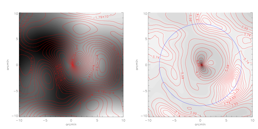
Figure 2: Left panel: Simulated CMB temperature map with overlaid iso-contours of the temperature distortion caused by the lensing effect of a single galaxy cluster. Right panel: Convergence estimated with the non-linear filter described in the text. The background grey-scale map has a linear scale, while the iso-contours are spaced logarithmically. The circle represents the virial radius of the cluster. The maps show results for an ideal instrument without noise and a resolution of $4.68$ arc sec. Note that the reconstructed convergence shows a spurious elongation perpendicular to the local CMB gradient, which arises because the lensing effect on the CMB vanishes in this direction.

4 Data analysis: Application of the filter

We demonstrate in this Section the filter’s capability to recover the convergence by first applying it to a single cluster in the ideal case without any instrumental noise (Subsect. 4.1) and then including the kSZ effect (Subsect. 4.2).

In Subsect. 4.3, we investigate whether and how it will be possible with the data from the 225-GHz ACT channel to obtain average cluster convergence profiles. The assumed observing strategy is to detect clusters through their tSZ signal and then to suitably stack CMB maps surrounding them in order to enhance the signal-to-noise ratio. We shall assume that a total area of $200$ square degrees will be covered with ACT.

4.1 Convergence estimation for a single cluster

For studying the filter’s capability to recover the convergence of a single cluster, we applied our filter to a CMB map with $2048^{2}$ pixels simulated as described in Sect. 3. This CMB map was lensed with an axially-symmetric galaxy cluster model with NFW density profile and with a mass of $10^{15}\,h^{-1}\,M_{\odot}$ placed at redshift $0.3$. No instrumental noise was added yet.

The left panel of Fig. 2 shows the CMB temperature map with overlaid iso-contours of the temperature distortion pattern caused by the lensing effect of the cluster. The characteristic dipole pattern is clearly visible. The right panel of the same figure shows the estimated cluster convergence. The grey-scale map has a linear scale, while the iso-contours are logarithmically spaced. The circle illustrates the virial radius of the cluster.

Figure 3: The convergence profile of the input cluster is plotted as the solid line. The dots with error bars show the reconstructed mean convergence profile determined from 10, 100, and 1000 replications of the same cluster on different realisations of the CMB. The error bars were determined by bootstrapping the cluster sample. While the input profile is well reproduced outside a few scale radii, the reconstructed profile is too flat in the core.

Figure 3 illustrates the cluster profile reconstruction after a straightforward application of our filter. The input cluster, whose profile is plotted as the solid curve, is placed in front of 10, 100, and 1000 different realisations of the CMB. The filter is applied, and the radial profile of the convergence estimate $K(\@vec{\theta})$ is determined and averaged across the cluster sample. Outside a few scale radii, the reconstructed profile flattens because the clusters disappear in the CMB. While approaching the input profile outside a few scale radii until the noise begins dominating, the reconstructed profile is evidently too flat in the core. This can be overcome by introducing a suitably weighted average, as we shall now describe.

Note that the reconstructed convergence shows a spurious elongation perpendicular to the local CMB gradient, which arises because lensing of the CMB by a cluster has no effect in this direction (cf. Eq. 2). This degeneracy is thus characteristic for lensing of the CMB temperature anisotropy rather than the filtering technique applied. It could be broken only with some additional information, like lensing of the polarisation anisotropy.

This suggests to determine the convergence profile not by a straight average in azimuthal bins, but after multiplying the observed map with a weight map

$$P(\@vec{\theta})=|\@vec{G}(\@vec{\theta})|^{2}\cos^{2}\xi(\@vec{\theta})\;,$$ (16)

where $\xi(\@vec{\theta})$ is the angle between the CMB gradient and the deflection field at the position $\@vec{\theta}$, under the assumption that it has radial symmetry. This is exact for our axially-symmetric analytical cluster model, but it can also be applied to the general case of asymmetric clusters because the deviation of the deflection-angle direction from the radial symmetry is small even for substructured clusters. Assuming therefore that the deflection-angle points towards the field centre, we have

$$\cos\xi(\@vec{\theta})=-\frac{\@vec{\nabla}T(\@vec{\theta})}{|\@vec{\nabla}T(\@vec{\theta})|}\cdot\@vec{e}_{r}=-\frac{\@vec{G}(\@vec{\theta})}{|\@vec{G}(\@vec{\theta})|}\cdot\@vec{e}_{r}$$ (17)

where $\@vec{e}_{r}$ is the radial unit vector. Note that we have used the Wiener-filtered temperature gradient $\@vec{G}(\@vec{\theta})$ introduced in Eq. 4 which has its noise component minimised.

Using $P(\@vec{\theta})$, we determine radial weight profiles $P_{i}(\theta)$ for each cluster $i$ by averaging azimuthally,

$$P_{i}(\theta)=\theta\int_{0}^{2\pi}\mathrm{d}\varphi P_{i}(\@vec{\theta})\;,$$ (18)

and then determine the averaged convergence profile across a cluster sample,

$$\langle\kappa\rangle(\theta)=\frac{\sum_{i}\kappa_{i}(\theta)P_{i}(\theta)}{\sum_{i}P_{i}(\theta)}\;.$$ (19)

Figure 4: True and reconstructed cluster convergence profiles are shown as in Fig. 3, but now using the weighted profile average described in the text. The profile is now accurately reproduced well into the cluster core. Averaging over 100 clusters, the profile is detected out to approximately ten scale radii, or roughly twice the virial radius.

As in Fig. 3 for the unweighted average, Fig. 4 shows the recovered cluster convergence profiles obtained after weighting the average as described in (19). Well into the cluster core, the profile is now accurately reproduced. Averaging over a sample of 100 clusters, the profile is detected out to approximately ten scale radii, roughly corresponding to two virial radii. In view of the persisting uncertainty of central cluster density profiles, it is promising that the slope of the core profile is accurately reproduced even from ten clusters only.

Clusters which happen to be superposed on extrema or saddle points of the CMB temperature contribute little or nothing to the average lensing signal. The weighting scheme introduced here takes this automatically into account by reducing their statistical weight according to the signal they contribute.

The power of this filtering method is evident and opens a new technique for analysing data from the next-generation, high-resolution sub-millimetre observatories like ALMA.

Figure 5: Cluster convergence profiles as recovered by Hu’s (2001) original filter (long-dashed curve) and our modification of it (short-dashed curve). The input profile is shown as the solid curve. Both reconstructed profiles are weighted averages over 100 clusters.

Hu (2001) originally proposed his filter for recovering the deflection-field of the large-scale structure. In order to filter for clusters, our modification (8) of the weight map $W(\@vec{\theta})$ is crucial because introducing the factor $l$ increases the filter’s sensitivity on small scales. As Fig. 5 shows, the resulting effect is dramatic. While Hu’s filter certainly detects the cluster, but fails in recovering its profile, our modified filter faithfully reproduces the input profile over almost two orders of magnitude in the radius.

4.2 Adding the kinetic Sunyaev-Zel’dovich effect

As described, this non-linear filtering procedure was optimised for filtering out the uncorrelated Gaussian noise, like the CMB itself, instrumental noise and residuals from foreground subtraction, but it turns out to be also quite powerful in filtering out the contribution from the kSZ effect. The latter has a characteristic which could lead to future further improvements, as we shall clarify below.

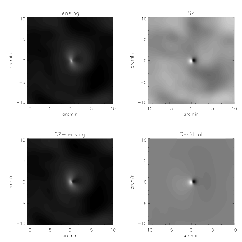
Figure 6: Processing of the kSZ effect: Results are shown for the cluster convergence reconstructed from a CMB field, to which only the lensing effect (top-left panel), only the kSZ effect (top-right panel), and the combination of both (bottom-left panel) was applied. The difference between the convergences recovered from the lensed CMB map and from the lensed CMB map with kSZ effect is shown in the bottom-right panel. The kSZ effect is processed like lensing by a hypothetical object with positive and negative convergence. The figure shows that the kSZ effect is well suppressed by the filter.

In order to understand how the filtering procedure processes the kSZ effect, we analysed a simulated map consisting only of the CMB and the kSZ effect. The result is shown in the top-right panel of Fig. 6. The top-left panel shows the same realisation of the CMB lensed by a cluster, the bottom-left panel combines both top panels, and the difference between the bottom-right and top-right panels is displayed in the bottom-right panel. The kSZ effect introduces an artefact in the recovered convergence field which has a maximum amplitude of only one tenth of the lensing signal and is characterised by a dipolar structure aligned with the CMB gradient, along which the lensing effect is also the strongest. Azimuthally averaging the recovered convergence, and stacking many cluster fields with random intrinsic orientations of the CMB gradient, further suppresses the kSZ signal in the lensing reconstruction.

Figure 7: Comparison of the recovered convergence profiles ignoring and including the kSZ effect (points with long- and short-dashed error bars, respectively). The solid curve shows the input cluster profile. Due to the various reasons detailed in the text, the kSZ effect leaves the lensing reconstruction essentially unaffected.

The dipolar pattern in the recovered convergence is caused by the fact that the filter interprets the entire secondary anisotropy as a lensing signal, and mimics it with a hypothetical lens with two adjacent positive and negative convergence peaks. Such a lens has a deflection-angle field reminiscent of an electric dipole, leading to a temperature signature identical to that of the kSZ effect. This peculiarity of the characteristic kSZ pattern could be used to further improve the filter including criteria for simultaneously minimising the kSZ effect.

Figure 7 illustrates the recovery of the cluster convergence profile in presence of the kSZ effect. Both curves with error bars were obtained placing the same cluster in front of 100 CMB realisations each and determining the weighted convergence profile as before. Evidently, the kSZ effect does not affect the lensing reconstruction in any significant way.

Figure 8: Relative deviation of the recovered cluster convergence profile averaging over three samples of 100 clusters each. The results were obtained weighting the average, ignoring or including the kSZ effect (solid and long-dashed error bars, respectively), and ignoring the kSZ effect and not weighting the average (short-dashed error bars). Weighting the average, the average profile is recovered to better than 10% near the scale radius.

Summarising this section, we show in Fig. 8 the relative deviation of the reconstructed cluster convergence profiles for three samples of 100 clusters each, without and with weighting the average, and without and with the kSZ effect included. Employing the weighted average, the recovered convergence is accurate to better than ten per cent near the scale radius, irrespective of the kSZ effect.

4.3 Example: Application to the cluster sample expected from ACT

For this Section, we simulated Gaussian CMB maps, including the lensing and the kSZ signal of clusters detectable through their tSZ effect, and also including the instrumental effects as explained in Sect. 3. We set the noise level to $6\,\mu\mathrm{K}$, and convolved the maps with a Gaussian beam with $1^{\prime}$ FWHM in order to investigate the expectations for estimating the average cluster convergence profile using data from the 225-GHz ACT channel.

We model the distribution of galaxy clusters in mass and redshift according to the mass function proposed by Sheth & Tormen (1999, 2002). Since galaxy clusters are detected through their tSZ effect at millimetre and sub-millimetre wavelengths, we truncate the cluster distribution where the solid-angle integrated Compton parameter $Y$ falls below a threshold

$$Y_{\mathrm{min}}=\frac{\Delta T}{T}\frac{\delta\Omega}{2}\;,$$ (20)

where $\Delta T/T$ is the instrumental sensitivity expressed in relative antenna temperature fluctuations, and $\delta\Omega$ is the effective solid-angle of the beam (Bartelmann, 2001). We choose $Y_{\mathrm{min}}=6.6\times 10^{-6}$ to approximate the sensitivity of the 225 GHz channel on ACT of $\Delta T/T=6\,\mu K$ and an angular resolution of $1^{\prime}$. We model the cluster distribution in the mass range from $10^{13}\,h^{-1}\,M_{\odot}$ to $10^{15}\,h^{-1}\,M_{\odot}$ between redshifts $0.01$ and $3$, obtaining in total $\approx 25000$ clusters. We assume that any foreground contamination can be removed with sufficient accuracy on a survey area of 200 square degrees. It is illustrated in Fig. 9.

Figure 9: The distribution of the galaxy-cluster sample used for this study is shown in the mass-redshift plane. The detection limit imposed by the ACT instrumentation is well visible as the sharp lower cut-off. The contours show the number density of detectable clusters per unit mass and redshift. They range from $(10^{-10}-5\times 10^{-10})\,hM_{\odot}^{-1}$ spaced by $5\times 10^{-11}\,hM_{\odot}^{-1}$.

In order to simulate the measurement error in the cluster positions on the sky, we randomly perturb their positions about the field centres by an amount drawn from a Gaussian distribution with a FWHM of one tenth of the angular resolution.

We apply the described technique to sets of CMB maps lensed by a cluster and superposed with the kSZ effect and instrumental noise, then compute the final weighted average convergence with the weight described in Eq. (16). Because of the poor resolution of cluster cores, the weighting scheme does not noticeably improve the results in this example, thus we show the unweighted results only.

Figure 10: Mass distribution of the clusters detectable for ACT. The lower mass cut-off is defined by beam smoothing and the detector sensitivity, the steep decrease towards high masses is due to the exponentially decreasing cluster mass function. The distribution peaks at $M\sim 5\times 10^{13}\,h^{-1}M_{\odot}$ and falls by one order of magnitude within $M\sim 4\times 10^{13}\,h^{-1}M_{\odot}$ and $M\sim 1.2\times 10^{14}\,h^{-1}M_{\odot}$.

Figure 11: Unweighted average estimated convergence obtained for the full simulated ACT cluster sample.

The sharp lower cut-off in the mass shown in Fig. 9, and the exponential upper cut-off due to the steep cluster mass function, leads to a very sharp peak in the distribution of clusters detectable for ACT (cf. Fig. 10). Also, the redshift distribution of the ACT cluster sample peaks near redshift unity, where the angular-diameter distance is almost independent of redshift. Averaging cluster profiles across the entire ACT sample is thus not expected to smooth the resulting profile by more than the beam smoothing. The result is shown in Fig. 11.

Figure 12: Unweighted mean convergence profile of a subsample of the clusters expected to be detected by ACT. The subsample was defined by requiring that the integrated Compton-$Y$ parameter falls within $7\times 10^{-6}\leq Y\leq 7.5\times 10^{-6}$.

Lacking information other than that derived from the tSZ effect, subsamples may be defined by imposing thresholds on the integrated Compton-$Y$ parameter. As an example, we show in Fig. 12 the unweighted mean profile of those clusters detected by ACT which have $7\times 10^{-6}\leq Y\leq 7.5\times 10^{-6}$. While the sample is now much better defined, the error bars increase considerably because of the much reduced number of clusters (2300 instead of 25000).

The instrumental resolution of $1^{\prime}$ is not small compared to the cluster size. Thus, most information is contained within a few resolution elements. This is evident in the reconstructed profiles of Figs. 11 and 12, where the measured points fall below the input profile within $1^{\prime}$, but well on the curve at larger radii. This implies that cluster mass estimates will suffer from the low resolution. The mean cluster mass determined from the mean convergence profile is typically a factor of two below the true mass of the input clusters. The lensing convergence can be converted to mass assuming a source redshift of $1100$, and adopting the mean redshift of the ACT clusters for the lens redshift.

5 Conclusions

Starting from a non-linear filter proposed by Hu (2001) for recovering the deflection-angle field of the large-scale structure from CMB temperature fluctuations, we have constructed a non-linear filter for extracting cluster-lensing signals from CMB maps. On the angular scales of galaxy clusters, the CMB is almost feature-less and can approximately be represented as a temperature gradient. Cluster lensing imprints a characteristic pattern on that gradient, which can be filtered for.

Since the signal obtained from a single cluster field will be weak, current instrumentation requires stacking many cluster fields in order to enhance the signal-to-noise ratio. Future instruments like ALMA may allow the lensing signal of individual clusters to be detected. Linear filtering would produce a signal aligned with the CMB gradient, so that the signal would be removed when averaging over cluster samples. Although other solutions are possible, this argues for a non-linear filter which effectively squares the signal.

Hu (2001) suggested to first take the Wiener-filtered temperature gradient, high-pass filter it in order to remove large-scale noise, take the divergence of the filtered gradient and normalise it such as to be proportional to the deflection-angle field. In order to detect small-scale cluster-lensing signals, we suggest to modify this procedure by shifting the high-pass filter to even higher frequencies, and to normalise the procedure such that the lensing surface-mass density, or convergence, will be recovered instead of the deflection-angle field. This has the further advantage of decaying much more rapidly away from cluster cores, which helps in applying fast-Fourier techniques.

We tested this non-linear filter under various assumptions. First, we showed that cluster convergence profiles are reasonably recovered from stacked cluster fields. Azimuthally averaging cluster fields, and averaging the resulting profiles, reproduces the input cluster convergence profile quite well, but the recovered profiles are too shallow in the core.

As the reason for that deviation, we identified the fact that the lensing signal is weak or absent in directions approximately perpendicular to the CMB temperature gradient. We thus introduced a weighting scheme for each individual cluster field which quantifies the alignment of the lensing deflection with the CMB gradient, and down-weights the signal in proportion to the cosine of the angle between the lensing deflection and the temperature gradient. Directions perpendicular to the temperature gradient and flat areas in the temperature map, along which and where the lensing signal vanishes, are thus effectively removed. Weighting the average of the recovered cluster profiles in that way substantially improves the agreement with the input profile. We found that an average over 100 cluster fields excellently recovers the mean cluster profile out to several scale radii, and detects it significantly beyond the virial cluster radius.

This filter is best applied on data taken at frequencies near 217 GHz in order to suppress noise introduced by the tSZ effect. The kSZ effect, however, cannot be avoided in that way. From the point of view of gravitational lensing, the kSZ effect can be mimicked by a dipolar lens consisting of a positive and a negative mass contribution. Filtering lensed CMB data including the kSZ effect thus adds a further source of noise to the recovered density profile. Including that in our simulations, we found however that the kSZ effect affects the results by a negligibly small amount. The three main reasons for that are that the specific dipolar signature of the kSZ effect tends to average away by stacking cluster fields, that mean radial cluster velocities also average to zero across a cluster sample, and that the spurious lensing signal produced by the kSZ effect is approximately one order of magnitude below the true lensing signal.

Finally, we tested what can be expected from filtering the data to be obtained from the Atacama Cosmology Telescope (ACT) for cluster lensing. Given ACT’s angular resolution of $1^{\prime}$, cluster lensing signals can only be detected in the innermost resolution elements surrounding the cluster cores. It will thus only be possible to recover mean cluster convergence profiles outside of $1^{\prime}$, and mean cluster masses will be underestimated. Those simulations took the instrumental noise expected for ACT’s 225-GHz detector into account.

These results are particularly encouraging in view of upcoming wide-field sub-mm surveys to be carried out with telescopes like APEX and ALMA. It appears realistic that non-linear filtering will allow mean cluster convergence profiles to be reliably recovered from their gravitational-lensing signature.