Star–disc interactions in a galactic centre and oblateness of the inner stellar cluster

Abstract

Structure of a quasi-stationary stellar cluster is modelled assuming that it is embedded in the gravitational field of a super-massive black hole. Gradual orbital decay of stellar trajectories is caused by the dissipative interaction with an accretion disc. Gravitational field of the disc is constructed and its effect on the cluster structure is taken into account as an axially symmetric perturbation. Attention is focused on a circumnuclear region ($r\la 10^{4}$ gravitational radii) where the effects of the central black hole and the disc dominate over the influence of an outer galaxy. It is shown how the stellar system becomes gradually flattened towards the disc plane. For certain combinations of the model parameters, a toroidal structure is formed by a fraction of stars. Growing anisotropy of stellar velocities as well as their segregation occur. The mass function of the inner cluster is modified and it progressively departs from the asymptotic form assumed in the outer cluster. A new stationary distribution can be characterized in terms of velocity dispersion of the stellar sample in the central region of the modified cluster.

1 Introduction

We discuss the impact of gaseous environment on the long-term stellar motion in central regions of active galactic nuclei (AGN). We adopt the view of galactic nuclei as composite systems with stars surrounding a super-massive black hole (with a typical mass of $10^{6}M_{\sun}\la M_{\bullet}\la 10^{9}M_{\sun}$) and forming a rather dense cluster (Begelman & Rees 1978; Norman & Silk 1983). Central number density of the cluster stands as one of the model parameters that can reach values of the order of $n_{\ast}\sim 10^{6}\div 10^{7}\,\mbox{pc}^{-3}$. We consider the stars of the cluster as satellites orbiting the central black hole. We also take into account the influence that the diluted interstellar environment exhibits on the motion of stars on time-scales exceeding $10^{4}$ dynamical periods. This allows us to address an important question whether or not the presence of such medium could increase the concentration of stars in certain regions of the nucleus.

Although we consider the region of direct gravitational influence, where the gravity of the central black hole dominates over non-gravitational forces, one should not neglect the impact of perturbing effects on individual stellar trajectories and the overall cluster structure. We assume that it is the gas in an accretion disc which acts as the main perturbation. The disc medium affects the motion of stars either directly by collisions between stars and gas particles at the point of transition through the disc slab (the case of inclined trajectories), or vicariously, via coupling between the stars and the disc medium (embedded trajectories). These processes will be discussed in combination with the effects of disc gravity.

Our present contribution follows a previous paper (Vokrouhlický & Karas 1998) where the long-term evolution of stellar orbits was studied including the case of an axially symmetric perturbation imposed on the gravitational field to mimic the presence of a disc. It was shown that the orbits experience abrupt changes of eccentricity and inclination even if the disc mass is a tiny fraction of the central mass, $M_{\rm{}d}\la 10^{-3}{M_{\bullet}}$. In that paper properties of individual orbits were investigated. A simplified approach to the evolution of the central cluster was adopted in Rauch (1999) and Karas, Šubr & Šlechta (2002). Stellar encounters were explored in this context by Vilkoviskij & Czerny (2002), using a semi-analytical approach to the dense and flattened cluster. Here we add an astrophysically more realistic description of the self-gravitating disc, especially of its gravitational field that superimposes with the central field, and we study dynamics of the cluster in terms of its overall characteristics (the shape and velocity dispersion).

The main new ingredients of the present investigation are threefold. Firstly, a more elaborate description of the disc accounts for different processes and corresponding time-scales that dominate the system evolution at different distances from the core. Orbit behaviour is governed mainly by the overall radial profile of the disc (especially its surface density and vertical thickness) and by stellar characteristics (mass and size). The interplay between these principal parameters determines the hydrodynamical mechanism driving the evolution – collisions with the disc, density waves, or formation of gaps in the disc.

Secondly, we introduce the distribution of stellar masses in the cluster, ${\cal{N}}(M_{\ast})$. The cluster is supplied with a Salpeter type initial mass function, but the resulting mass function is eventually different because of selective orbital decay. For our purposes, stars are characterized phenomenologically by their effective column density $\Sigma_{\ast}{\equiv}M_{\ast}/\left({\pi}R_{\ast}\right)^{2}$ as a key paramater that rules this effect.

Thirdly, we consider the distribution of stars in phase space. Simulations start with a spherically symmetric and stationary cluster whose dynamics is dominated by the central black hole mass (Bahcall & Wolf 1976, BW hereafter). This solution describes a gravitationally relaxed system of stars near a black hole with phase-space probability density $f_{0}(a)\,\propto\,a^{1/4}$ ($f_{0}(a)\,{{\mbox{d}}}a$ is the number of stars in a shell with semi-major axis $a$ and width ${{\mbox{d}}}a$). We assume that the modified distribution approaches $f_{0}(a)$ far away from the core, but it can be modified in the inner parts of the system where also the importance of the disc increases. Other self-consistent models have been discussed for a cluster with a central black hole (e.g. Young 1980; Quinlan, Hernquist & Sigurdsson 1995; Takahashi & Lee 2000; Alexander 2003) for which the radial density profile turns out to be different but also a power-law type at large radii. Furthermore, several authors (e.g. Rauch 1995; Freitag & Benz 2002; Alexander & Hopman 2003) have developed numerical approaches taking stellar collisions into account in a dense cluster near a black hole.

The paper is organized as follows. In the next section we describe the ingredients of the model and time-scales involved. In Section 3, we show a modified quasi-stationary stellar distribution that emerges in the inner regions of the cluster. We discuss transition regions where the stars are gathered and we also examine predicted velocity dispersions, mean spectral-line profiles and the modified mass function. Some of these properties may have direct observational consequences. Finally, limitations of the model are discussed and conclusions are presented in Section 4.

2 The model

2.1 Components of the model

Our exploratory model is based on a presumably obvious assumption of dissipative processes prevailing in the center, where the disc surface density is high, while gravitational relaxation is supposed to be in control on the outskirts of the system behind the outer edge of the disc. The adopted approach contains simplifications that help us to proceed in the situation when $N$-body or equivalent methods are still a challenge, especially if the dissipative environment, different types of stars and non-spherical geometry of the system are to be taken into account. The model consists of three components:

(a)

A super-massive black hole. Its influence is approximated by Newtonian gravitational field of a point mass $M_{\bullet}$. Relativistic effects are introduced only by adopting ${R_{\rm{}g}}{\equiv}G{M_{\bullet}}/c^{2}\sim 1.5\times 10^{13}\,M_{8}\,\rm{cm}$ ($M_{8}{\equiv}{M_{\bullet}}/10^{8}M_{\sun}$) as the smallest natural length-scale that appears in our considerations. The corresponding dynamical time-scale is much shorter than all other time-scales in the model and it does not stand explicitely in equations of the long-term evolution hereafter.

(b)

An accretion disc. In order that computations be well defined and easier to compare, we consider the standard Shakura–Sunyaev disc (denoted as “SS”; e.g. Frank, King & Raine 2002) and a model of weakly self-gravitating disc (Goldreich & Lynden-Bell 1965; Paczyński 1978; Shlosman & Begelman 1989). We assume that approximation of vertically averaged quantities is sufficient for our analysis and we characterize the disc by surface density $\Sigma_{\rm{}d}(r)$ and geometrical semi-thickness $H(r)$ (functions of radius in the disc mid-plane $z=0$). Other variables are also relevant for star–disc interactions, e.g. radial velocity of mass transport in the disc, temperature of the medium and speed of sound. Gravitational field is determined numerically. With the disc we associate time-scale $t_{\rm incl}$, i.e. the interval on which stellar orbits are inclined into the plane by the dissipative interaction.

(c)

A nuclear cluster. It is characterized by the distribution function $f_{\ast}$ that conforms initially to a spherically symmetric and stationary state in the central potential well. In our computational scheme, the cluster is divided in two distinct subsets that are treated separately. In the inner cluster, the stellar system becomes oblate and anisotropic due to the dissipative interaction with the disc. Efficiency of this interaction depends on the parameters of individual stars and, therefore, it is sensitive to their masses, orbital inclinations, as well as to properties of the dissipative environment. Gravitational relaxation is neglected in the inner cluster, assuming that $t_{\mbox{\scriptsize r}}\gg t_{\rm incl}$. The outer cluster, on the other hand, does not evolve in our computations and its structure is determined by gravitational relaxation as a dominating process. The outer cluster acts as a reservoir from which fresh stars are injected inwards, maintaining the overall steady state.

Figure 1: Gravitational field of different models of a disc is shown in comparison with the central field of the black hole. Ratio of the corresponding field components was computed and the resulting contours plotted (in azimuthal section). The ratio of vertical ($z$) components is shown in the top row (i.e. $F_{z,\rm{}disc}/F_{z,\rm{}centre}={\rm{}const}$), while the ratio of radial (cylindrical $R$) components is in bottom ($F_{R,\rm{}disc}/F_{R,\rm{}centre}={\rm{}const}$). Obviously, near the equatorial plane the vertical component of the disc gravity dominates. Three representative types of discs have been selected for illustration, as indicated above the frames. Contours are drawn in logarithmic spacing and the values refer to $\mu=1$.

2.2 An accretion disc with effects of self-gravity

We adopt three flavours of the standard model: (i) radiation pressure dominated standard (SS) disc; (ii) gas-pressure dominated SS disc with electron scattering; and (iii) the same as the previous case but with free-free opacity (Frank et al. 2002). Radial dependence of the disc variables is expressed by power-law in all those cases, in particular, the surface density can be written in the form $\Sigma_{\rm{}d}/\Sigma_{\ast}\,\propto\,\left(r/{R_{\rm{}g}}\right)^{s}$. The values of index $s$ are given in Table 1 for different cases (see also Karas & Šubr 2001) and we will introduce also non-powerlaw profiles later in this section.

Table 1: Values of the power-law index $s$ characterizing the radial dependency of the disc surface density $\Sigma_{\rm{}d}(r)$.

Model	(i)	(ii)	(iii)	(iv)	(v)
$s$ parameter	$3/2$	$-3/5$	$-3/4$	$-15/7$	$-5/3$

The standard scheme was supplemented by considering self-gravity according to Collin & Huré (1999, 2001) and Huré et al. (1994, 2000). Based on Toomre’s criterion ($Q\sim 1$) for onset of self-gravity, AGN accretion discs are affected beyond critical radius $\sim 10^{3}{R_{\rm{}g}}$ (i.e. $\sim 0.01$ pc, depending on model parameters). Farther out, at $\ga 1$ pc from the center, the disc mass can reach a sizeable fraction of the central mass. For example, the mass ratio of the disc (ii) with respect to the central mass is $\mu\equiv M_{\rm{}d}/M_{\bullet}=0.3M_{8}^{6/5}\dot{M}_{0.1}^{3/5}\alpha_{0.1}^{-4/5}\left(R_{\mbox{\scriptsize d}}/10^{5}{R_{\rm{}g}}\right)^{7/5}$ where we $R_{\mbox{\scriptsize d}}$ is the disc outer radius, $\dot{M}_{0.1}=\dot{M}/0.1\dot{M}_{\rm{}Edd}$, $\alpha_{0.1}=\alpha/0.1$. Similarly, for case (iii) we have $\mu=0.1M_{8}^{6/5}\dot{M}_{0.1}^{7/10}\alpha_{0.1}^{-4/5}\left(R_{\mbox{\scriptsize d}}/10^{5}{R_{\rm{}g}}\right)^{5/4}$, suggesting that the disc attraction is strong enough to influence the motion of stars independently of the details of a particular model. Self-gravity manifests itself by gathering material to the mid-plane, thereby narrowing vertical thickness.

We considered the case of marginally stable self-gravitating discs. Two examples, denoted as (iv) and (v) hereafter, are characterized by $Q\sim 1$ and they differ by assumption about elemental abundances: solar metalicity is adopted in the case (iv) while it is set to zero in the case (v). Because of differences in opacities, different density profiles and values of the total disc mass are obtained. Typically, in the outer region of a marginally stable disc, density decreases faster compared to the standard case. For a detailed discussion of the adopted models, see Huré (2000) and references cited therein.

Finally, we considered composite discs, by which we mean a combination of simple models. For example, case (ii)+(iv) is constructed by concatenating two corresponding basic models. Notation indicates that the standard SS disc (ii) is assumed at small radii and matched to a marginally self-gravitating disc (iv) at large distance from the centre (density and other variables are continuous at the transition radius). This approach reflects an obvious fact that simple models can be valid only for a limited range of radius and provides setup for the model that is rich enough to capture different possibilities.

Figure 1 illustrates three examples of the structure of the gravitational field. To this aim we plot the ratio of field components that correspond to the disc and to the central black hole (contribution of the cluster stars is not included in this figure). Different frames reveal the difference between the case of Kuzmin’s disc (employed in Vokrouhlický & Karas 1998) and two typical examples of our discs, computed numerically for this paper. Even if the gravitational field of the disc is perturbative ($\mu\ll 1$), it turns out that the vertical component of the disc field may successfully compete with that of the centre in certain regions near the disc plane. This is essential not only for the disc internal structure but we can also expect stellar paths to be visibly dragged (on the long term), especially those which follow a low-inclination orbit, i.e. almost embedded in the disc.

The gravitational potential and the field due to disc are computed according to Poisson’s integrals in which integrations are carried over volume occupied by the gas, assuming axial symmetry. We used the splitting method for accurate evaluation (Huré 2000). Furthermore, in order to reduce duration of runs, we implemented a dynamical grid in the Poisson solver and we pre-generated the field components in a Cartesian grid covering a rectangular region of 1 pc $\times$ 1 pc. In some regions, close to the disc, the field lines are very distorted. We found it convenient to define additional sub-grids which provide fine resolution where needed. Field values between mesh points were obtained by bilinear interpolation. Hereafter, we will illustrate results for discs (iii) and (ii)+(iv), i.e. the same as in Fig. 1. These two cases appear sufficient in order to demonstrate various stages of the modified cluster. The models share the same black hole mass, $M_{\bullet}=10^{8}M_{\sun}$, as well as other common parameters of the disc: $R_{\mbox{\scriptsize d}}=10^{4}{R_{\rm{}g}}$, $\dot{M}=0.1\dot{M}_{\mbox{\tiny E}}$, and $\alpha=0.1$. Corresponding mass ratio is $\mu=1.2\times 10^{-2}$ and $\mu=2.9\times 10^{-3}$ for discs (iii) and (ii)+(iv) respectively.

Figure 2: Long-term evolution of orbital elements for a single star. Different modes of star–disc interaction are distinguished by line type in the graphs, corresponding to the three subsequent phases of the mean motion (details in the text): in phase 1 the regime of direct collisions takes place (solid line); in phase 2 the regime of density waves occurs, in which $a$ drops more rapidly (dashed line); finally, phase 3 describes migration of a star tidally coupled to the disc (dotted line). Time is scaled with respect to the initial dynamical period, $T_{0}=2\pi\sqrt{GM_{\bullet}}\,a_{0}^{3/2}$; semi-major axis is expressed in terms of the initial $a_{0}$.

2.3 Star–disc interactions

Stars passing through the disc may create gaps and holes in some regions, but we assume that the disc is not removed completely, implying that the accretion rate cannot be too low and the cluster excessively dense. We adopt the approximation of impulsive (i.e. instantaneous) interaction between crashing stars and the disc (Syer, Clarke & Rees 1991; Karas & Vokrouhlický 1994). In this way, stellar trajectories slowly evolve and several phases can be distinguished in the course of orbital evolution.

During the initial phase, as long as the stars are crashing on the disc with non-zero inclination, the following combinations of orbital elements $a$, $x\equiv\cos{i}$ and $y\equiv(1-e^{2})$ remain constant:

$$C_{1}=a\,y\,(1+x)^{2}\quad\mbox{and}\quad C_{2}=\frac{(1-y)(1+x)^{3}}{1-x}$$ (1)

(see Šubr & Karas 1999). These two conserved quantities can be employed to determine the orbital evolution along with a simple estimate of $t_{\rm incl}$,

$$t_{\rm incl}=t_{0}M_{8}\,\frac{\Sigma_{\ast}}{\Sigma_{\sun}}\left(\frac{a_{0}}{{R_{\rm{}g}}}\right)^{3/2-s}\,{\rm yr}\,.$$ (2)

Here, various model-dependent factors were absorbed in the term $t_{0}{\equiv}t_{0}(a_{0},e_{0},i_{0})$ that varies only slightly with $a_{0}$. For example, in cases (ii), …, (v), and for $e_{0}=0$, $i_{0}=\pi/2$, we find $t_{0}=0.92$, $0.22$, $1.89\times 10^{-6}$ and $9.40\times 10^{-4}$, respectively (these numbers were determined numerically). Because there is considerable uncertainty in the actual value of the disc surface density and since the cluster consists of various stellar types, ranging from compact stars to giants, it is easy to realize that $t_{\rm incl}$ must span an enormous range over seven orders of magnitude in eq. (2).

Inclination and eccentricity decay exponentially at late stages when $i\propto\exp[-t/\tau]$, $e\approx\sqrt{C_{2}}/(4i)$, while the semi-major axis slows down and eventually reaches its asymptotical value $a_{\mbox{\scriptsize f}}=C_{1}/4$. When inclination drops to a critical value (given by $\tan{i}{\sim}H(r)/r$), the regime of direct collisions goes over to the regime of stars entirely embedded in the disc. Since this moment, we further distinguish two modes of inward migration through the disc medium. If the stellar mass is large enough to create a gap (e.g., Lin & Papaloizou 1986), the star becomes tidally coupled with the disc and it sinks to the centre at roughly the same rate as the material of the disc. Otherwise, excitation of density waves dominates and causes radial migration to be faster, typically by order of magnitude (Ward 1986; Artymowicz 1994).

In Figure 2 we show a particular case of an orbit evolving with the disc (iii) and $M_{\ast}=3M_{\odot}$, ensuring that the star successively enters all three modes of migration. Starting from $a_{0}=10^{3}{R_{\rm{}g}}$, $e_{0}=0.45$ and $x_{0}=0.54$, the semi-major axis converges to $a_{\mbox{\scriptsize f}}=0.47a_{0}$ along with the simultaneous decay of eccentricity and inclination. The initial phase of star–disc collisions is followed by the decay due to density waves. Finally, as the disc parameters change with radius, the star eventually clears a gap in the disc and the dominant mode of its radial migration is switched once more.

Figure 3 illustrates an interesting effect that emerges once the gravitational field of the disc is taken into account. The disc introduces a non-spherical perturbation to the background gravitational field of the central mass. As a consequence, a Kozai-type mechanism causes occasional jumps of orbital parameters. A specific form of the disc gravitational field is not particularly crucial for the onset of these hops, but the dissipative orbital decay and appropriate arrangement of time-scales are important (see Vokrouhlický & Karas 1998 for more discussion). In fact, any non-spherical perturbation, for example general-relativity effects of frame-dragging near a rotating black hole, can potentially be responsible for similar kind of oscillations.

Figure 3: Similar to the previous figure, but for stars moving in superposed gravitational field of the central black hole mass and an axially symmetric thin disc. The spherical symmetry is now broken, bringing new features into the orbit evolution. Namely, sudden steps in the osculating elements occur at resonances between radial and vertical oscillation frequencies. Again, semi-major axis is scaled with respect to the initial value, $a_{0}$, and time is given in units of $T_{0}$ (only a part of the whole evolution is shown for better clarity). Short-term variations of the elements were filtered out in this graph.

In the following sections we discuss integral properties of the whole cluster, and therefore we will sum over individual stars. One should bear in mind that orbital resonances can set stars on very eccentric trajectory, increasing the capture rate. Hence the presence of the disc may influence the overall cluster structure in its inner regions.

2.4 The cluster

Stationary state is maintained by a continuous inflow of fresh stars from the outer reservoir and this is accomplished by distinguishing between two populations of orbits: those which belong to the relaxed cluster with a prescribed distribution $f_{0}$ and those which are influenced by the disc and belong to the inner cluster. The latter contribute by fraction $f_{0}\,t_{\rm incl}/t_{\mbox{\scriptsize r}}$. The cluster as a whole is superposition of these two populations; the corresponding distribution will be denoted $f_{\ast}$ hereafter. Because the influence of the disc on stellar orbits is greater at small distances and likewise the effect of circularization increases inwards, therefore the distinction between the two populations reflects also their spatial dimensions.

First we introduce the distribution $f_{0}(a_{0},e_{0},x_{0},\omega_{0})$, which characterizes the initial form of the cluster so far unperturbed by the disc. It is determined by relaxation processes, acting on time-scale

$$t_{\mbox{\scriptsize r}}=\frac{\sigma^{3}}{G^{2}C\ln\Lambda\,M_{\ast}^{2}n_{\ast}},$$ (3)

where $\sigma$ is the velocity dispersion, $n_{\ast}$ the number density of the stellar system, $\ln\Lambda$ is Coulomb logarithm and $C$ is a constant (in usual notation, $C\ln\Lambda\sim 10^{2}$; e.g. Spitzer 1987).

If relaxation was neglected in comparison with the dragging of stars by the disc, one could write probability of finding a star on an orbit with semi-major axis $a$ in the form

$$f_{\ast}(a;a_{0},e_{0},x_{0},\omega_{0})\,{{\rm d}}a={{\rm d}}\Omega\,f_{0}(a_{0},e_{0},x_{0},\omega_{0})\,t_{\mbox{\scriptsize r}}^{-1}J^{-1}\,;$$ (4)

where $J\equiv\|{\rm d}{}a(a;a_{0},e_{0},x_{0},\omega_{0})/{\rm d}{}t\|$ and ${\rm d}\Omega$ is the phase space element. Meaning of this relation can be clarified by integrating eq. (4) over $a$ and obtaining the total number of stars in the inner cluster which have been injected from ${\rm d}\Omega$. This number is equal to the fraction of stars in ${\rm d}\Omega$ multiplied by the ratio of drag period to the relaxation period. At the same time, integration over the phase space of initial parameters gives the desired probability density in the inner cluster:

$$f_{\mbox{\scriptsize in}}(a)\,{\rm d}a=\int_{\Omega}{\rm d}\Omega_{0}\,f_{0}(a_{0},e_{0},x_{0},\omega_{0})\,t_{\mbox{\scriptsize r}}^{-1}J^{-1}\,.$$ (5)

The way in which the boundary zone is introduced between the inner and the outer populations is the main advantage (and limitation) of the adopted approach. It is assumed that $\Omega$ is vacated solely by dissipative effects (interaction with the disc), while it is filled, at a constant rate, solely via relaxation. In the numerical scheme this is achieved by requiring $t_{\rm incl}$ to be shorter than relaxation time (3) in the outer cluster, i.e.

$$t_{\rm incl}\sim\frac{a_{0}}{|\dot{a}|}\leq t_{\mbox{\scriptsize r}},$$ (6)

where $\dot{a}$ is the rate of orbital decay (we substituted the value of $\dot{a}$ at initial time). Another condition is imposed by requiring that the orbit intersects the disc,

$$R_{\mbox{\scriptsize d}}>R_{0}\equiv\frac{a_{0}\,(1-e_{0}^{2})}{1+e_{0}\,\cos\omega_{0}}.$$ (7)

A Monte Carlo code was used to evaluate the integral on the right-hand-side of eq. (5). We followed $N\sim 10^{7}$ orbits with randomly generated starting values of osculating elements. Each time an orbit reaches a pre-determined value of $a_{i}$ (these are distributed in a logarithmical grid) the corresponding bin of the probability-density array is increased by factor $|\dot{a}|^{-1}$. This contributes by

$$f_{i}=\frac{1}{t_{\mbox{\scriptsize r}}}\frac{N_{0}}{N}\sum_{1}^{N_{\mbox{\tiny c}}}\left|\frac{{\rm d}a}{{\rm d}t}(a;{\mathbf{}r},{\mathbf{}v})\right|^{-1}\,$$ (8)

to the distribution. Here, $N_{0}$ is the total number of stars within the specified range of radii in the outer cluster, and $N_{\mbox{\scriptsize c}}$ is the number of generated orbits intersecting the disc and satisfying conditions (6) and (7). In typical calculation, $N_{\mbox{\scriptsize c}}$ reaches a few percent of $N$.

The code enables us to further distinguish two subsamples of the inner cluster. Stars on inclined orbits intersecting periodically the disc are counted to a dragged cluster. Once a star is embedded entirely into the plane of the disc and the mode of its radial migration is changed accordingly, we begin counting the star as a member of an embedded cluster. It turns out that these two subsamples populate different regions of the parameter space of the inner cluster, and so the distinction appears plausible.

We have employed the BW distribution to populate the outer reservoir. Maxwellian velocity distribution is used as a boundary condition specifying the dispersion $\sigma_{\mbox{\scriptsize c}}$ at zero binding energy surface. As mentioned above, $f_{0}(a_{0})\,\propto\,a_{0}^{1/4}$ with $a_{0}$ being within ${\langle}a_{\mbox{\scriptsize min}},a_{\mbox{\scriptsize max}}{\rangle}$. We set $a_{\mbox{\scriptsize min}}=R_{\mbox{\scriptsize d}}$ and $a_{\mbox{\scriptsize max}}=R_{\mbox{\scriptsize h}}$, where $R_{\mbox{\scriptsize h}}$ is radius of the black hole gravitational dominance,

$${R_{\rm{}h}}=G{M_{\bullet}}/\sigma_{\rm{}c}^{2}\sim 4.5M_{8}\sigma_{200}^{-2}\,{\rm pc},$$ (9)

written here in terms of $\sigma_{200}\equiv\sigma_{\rm{}c}/(200\,{\rm{}km\,s}^{-1})$. Remaining orbital parameters, $x_{0}$, $e_{0}$ and $\omega_{0}$, are distributed randomly with equal probability, ensuring spherical symmetry of the outer cluster. Corresponding spatial number density is

$$n_{\ast}(r)\sim(r/R_{\mbox{\scriptsize h}})^{-7/4}\,n_{0}\,.$$ (10)

The velocity dispersion of the BW cluster scales roughly as $\sigma^{2}{\sim}GM_{\bullet}/r$. With help of eqs. (9) and (10), relaxation time (3) can be rewritten as

$$t_{\mbox{\scriptsize r}}=10^{8}n_{6}\,M_{8}^{7/8}\biggl{(}\frac{M_{\ast}}{M_{\odot}}\biggr{)}^{-2}\biggr{(}\frac{r}{{R_{\rm{}g}}}\biggr{)}^{\frac{1}{4}}{\rm yr}$$ (11)

with $n_{6}\equiv(n_{0}/10^{6})\,$pc^-3.

Next, we need to specify a relation between $\sigma_{\rm c}$ and $M_{\bullet}$ that would hold outside $R_{\mbox{\scriptsize h}}$. We therefore adopt the empirical relation (Ferrarese & Merritt 2000; Gebhardt et al. 2000), $\log_{10}M_{8}=\alpha+\beta\log_{10}\sigma_{200}$ with $\alpha=0.13$ and $\beta=4$ (cf. Tremaine et al. 2002). In our model, the log-log formula for $\sigma_{\rm c}(M_{\bullet})$ is used to define the distribution of stars in the bulge overlaying our nuclear cluster and this way it unavoidably influences parameters derived from any observation. Otherwise, the forms of this relation in the two regions are quite independent of each other. Notice that simplicity is one of the reasons for adopting the BW outer cluster, but it is not necessary for the method as such. Likewise, different distributions of eccentricities can be accommodated. For example, we tested $f_{\ast}(e)\,\propto\,e$ and $f_{\ast}(e)\,\propto\,\exp(e)$ without much impact on the results, i.e. on the final distribution of the system.

The spatial size of the inner cluster is determined by the interplay between gravitational relaxation and dissipative effects in the disc. To estimate the size, two length-scales are naturally involved. Firstly, from eq. (7) it is the disc radius $R_{\mbox{\scriptsize d}}$ which limits the region of star–disc collisions. Secondly, we notice that $t_{\mbox{\scriptsize r}}(r)$ increases with radius at slower rate than $t_{\rm incl}(a)$. Hence, by substituting $a{\rightarrow}r$ and setting $t_{\mbox{\scriptsize r}}=t_{\rm incl}$ we define a characteristic radius

$$\left(\frac{R_{\mbox{\scriptsize i}}}{R_{\mbox{\scriptsize i${}_{0}$}}}\right)^{\frac{5}{4}-s}\!\!\!=n_{6}^{-1}M_{8}^{-1}\frac{\Sigma_{\ast}}{\Sigma_{\sun}}\left(\frac{M_{\ast}}{M_{\sun}}\right)^{-2}\left(\frac{R_{\mbox{\scriptsize h}}}{10^{6}{R_{\rm{}g}}}\right)^{-\frac{7}{4}}.$$ (12)

For our exemplary disc models, one finds the following values: (ii) $R_{\mbox{\scriptsize i${}_{0}$}}=4.73\times 10^{4}{R_{\rm{}g}}$, (iii) $4.36\times 10^{4}{R_{\rm{}g}}$, (iv) $1.68\times 10^{4}{R_{\rm{}g}}$, and (v) $9.80\times 10^{3}{R_{\rm{}g}}$. Eq. (12) is useful for analytical estimates of the cluster size. The smaller of the two radii $R_{\mbox{\scriptsize i}}$ and $R_{\mbox{\scriptsize d}}$ corresponds to the size of the inner cluster. This estimate is in agreement with numerical simulations.

Finally, we modified the above-described scheme and tested a model with the initial distribution $f_{0}$ being set to be Maxwellian in velocities. By comparing the results based on both approaches we found qualitative agreement between these two different formulations (see Karas et al. 2002 for details).

3 Results

3.1 Radial structure of the modified cluster

Figure 4: Typical examples of the structure of a cluster resulting from its interaction with different models of an accretion disc. Top panels: distribution $f_{\ast}(a)$ of stars (solid line, in arbitrary normalisation) residing in a shell of given semi-axis ($a$ in units of ${R_{\rm{}g}}$). Dashed, dotted, and dash-dotted lines stand for the three sub-components of the cluster, i.e. the embedded, dragged, and relaxed (outer) population. Bottom panels: mean orbital inclination ${\langle i\rangle}$ throughout the whole cluster, exhibiting the effect of flattening below $10^{4}{R_{\rm{}g}}$.

Let us first discuss the impact of star–disc interactions on the radial distribution of stars. Figure 4 provides connection between the properties of individual orbits and the overall evolution of the cluster. Parameters of the disc have been chosen identical as in Fig. 2, in particular, the outer edge $R_{\mbox{\scriptsize d}}=10^{4}{R_{\rm{}g}}$. Additional parameter is the stellar density, $n_{0}\sim 10^{6}{\rm{}pc}^{-3}$. In this case, radius $R_{\mbox{\scriptsize i}}$, defined by eq. (12), is approximately $2\times 10^{4}{R_{\rm{}g}}$, i.e. twice the disc outer radius. Therefore, the transition from the inner to the outer cluster occurs at $r=R_{\mbox{\scriptsize d}}$. Clearly, the transition area introduced in this way is not a sharp value of radius – it depends especially on eccentricity distribution of the stellar system, $R_{\mbox{\scriptsize d}}$ of the disc and $t_{\rm incl}/t_{\mbox{\scriptsize r}}$ of the both components. The resultant number density, $f_{\ast}(a)$, is closely matched by a broken power-law with a slope depending on the dominant regime of star–disc interaction. Notice that the asymptotic form is $f_{\ast}\propto\,a^{1/4}$ for large $a$.

Figure 5: Ratio $S(a;\mu)$ of two $f_{\ast}$ distributions obtained by considering or neglecting the gravity of the disc in computations. Two cases are shown in each panel: First, the gravitational field of the disc was computed in consistent manner with the disc surface density $\Sigma_{\rm{}d}(r)$ profile (solid line). Then, in order to demonstrate the dependency on the disc mass more clearly, we increased the $\mu$ parameter by factor of ten and recomputed the structure of the cluster with this new value (dashed line). The corresponding change of stellar density reaches order of several percent.

The impact of disc gravity can be demonstrated by “switching” the gravitational field of the disc on and off in computations. This is achieved by setting the value of $\mu$ parameter and computing the corresponding $f_{\ast}(a;\mu)$. In Figure 5, we show resulting ratios

$$S(a;\mu)\equiv\frac{f_{\ast}(a;\mu)}{f_{\ast}(a;\mu=0)}$$ (13)

of two such distributions. Each curve was obtained with two identical models, except for the inclusion or omission of the disc gravity. The two frames differ only by the adopted model of the disc. It turns out that perturbation to the stellar orbits by non-zero disc mass speeds up the orbital decay and, consequently, it decreases the number density of stars in the dragged cluster. This is visible even if the mass ratio is small, i.e. of the order of $\mu\sim 10^{-2}\div 10^{-3}$. Naturally, the influence of the disc gravity increases with $\mu$ increasing. Details of profile of the gravitational field also matter: we see, for example, that the disc (iii) affects $f_{\ast}$ more than the disc (ii)+(iv) if their mass parameter $\mu$ is comparable. The reason of this behaviour is that the former case has a flatter curve of $\Sigma_{\rm{}d}(r)$ (cp. Fig. 1) extending farther out from the black hole than the latter case, and hence it exhibits stronger impact on the cluster distribution.

Furthermore, we have included the orbital decay by gravitational radiation. Indeed, it is highly desirable to estimate this type of effects also because of forthcoming gravitational-wave experiments. We employed a simple approximation (Peters & Mathews 1963) and we found that gravitational radiation influences the final $f_{\ast}(a)$ only very near the centre (see Šubr & Karas 1999 for details). For the discs considered here, this occurs typically below $\la 10{R_{\rm{}g}}$ and, therefore, it does not leave any remarkable imprint on the results. Notice that this conclusion does not contradict the results of Narayan (2000) who considered case of low-density flows, and therefore he found the gravitational radiation to be more important for the orbital decay than the hydrodynamical dissipation, also at larger distance from the centre.

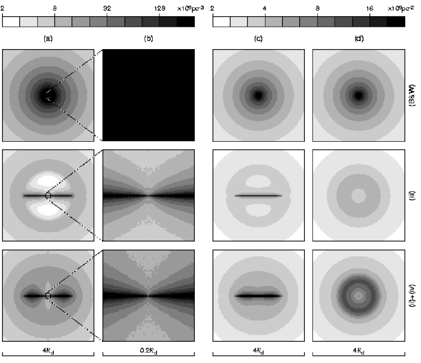
Figure 6: The spatial density $n_{\ast}(r)$ and the corresponding projected density of the cluster are shown using logarithmically spaced levels of shading. Columns (a) and (b) represent the meridional section at two different scales, namely, $4R_{\mbox{\scriptsize d}}$ and $0.2R_{\mbox{\scriptsize d}}$ across (radii are expressed in terms of the disc outer radius, $R_{\mbox{\scriptsize d}}$). Next columns are the edge-on (c) and the face-on (d) projections of the cluster. Across columns, the upper row shows the referential cluster ($n_{\ast}\,\propto\,r^{-7/4}$). In subsequent rows, the system has been already modified via the interaction with two types of discs, case (iii) and case (ii)+(iv), as indicated.

Because the system is non-spherical but axially symmetric and stationary, it is natural to portray its structure in a two-dimensional spatial projection. Figure 6 shows different sections of the cluster arranged in four columns. Starting from the left side, columns (a) and (b) represent the spatial number density $n_{\ast}(r)$ in the meridional plane across the cluster. Individual frames are centered on the black hole. Further, two columns on the right show the projected (column) density, i.e. the total number of stars integrated along the observer line of sight. Two different lines of sight were chosen, perpendicular to (c) and co-linear with (d) the symmetry axis. Interesting morphological patterns can be revealed by comparing different views.

Let us describe the meaning of individual rows of Fig. 6. In the first row, the density profile of the unperturbed BW distribution is plotted. It corresponds to the outer cluster which is clearly spherical and serves as a starting configuration for our computations. We show this case for the sake of comparison with the structure of modified clusters in subsequent rows. Again, we use the disc models (iii) and (ii)+(iv) as two representative cases.

Comparing different representations of the cluster one can clearly observe the impact that star–disc collisions have on the cluster structure. In particular, it is the increasing oblateness of the stellar population in the core and, in some cases, the tendency to form an annulus of stars. The effect is best seen in the bottom row in Fig. 6. However, details of the modified cluster structure obviously depend on the type of accretion disc that we choose. The reason of different structures stems from the different modes of radial transport of the stars from the cluster to the central hole. In the following paragraphs we examine several symptoms of the growing deformation of the cluster.

3.2 Anisotropy

The rate of dragging the stars by the disc is higher for counter-rotating stellar orbits than for co-rotating or aligned ones, hence, it is natural that the initial state of isotropy and sphericity becomes gradually violated. Less obvious is the fact that toroidal structures may be formed as a consequence. To see the effect we inspect graphs of mean inclination ${\langle i\rangle}(a)$ (bottom row of Fig. 4). The above-mentioned populations of cluster members are clearly distinguished, in particular, small values of ${\langle i\rangle}(a)$ indicate a flattened structure of the cluster with a population of disc co-rotating orbits at small $a$. While the outer cluster approaches an isotropic system (${\langle i\rangle}\rightarrow\pi/2$) for large $a$, the dragged cluster is clearly flattened to roughly a constant value of mean inclination, (${\langle i\rangle}\sim 0.2)$. It drops further in the embedded cluster where ${\langle i\rangle}\rightarrow 0$. This behaviour provides another substantiation for distinguishing different populations that form the cluster.

The limiting value of mean inclination can be derived by the following simple analytical argument (which agrees with the results of computations). Probability density of finding a body in ${\langle}a,a+{{\rm d}}a\rangle\times{\langle}x,x+{{\rm d}}x\rangle$ is

$$f_{\ast}(a,x) {\!\!\!\!}= {\!\!\!\!}\int{\rm d}a_{0}\,{\rm d}x_{0}\,{\rm d}y_{0}\,{\rm d}\omega_{0}\,\frac{f_{0}(a_{0},x_{0},y_{0},\omega_{0})}{t_{\rm r}(a_{0})}\left|\frac{{\rm d}a}{{\rm d}t}\right|^{-1}$$ (14)

$${\!\!\!\!}\times \delta\left(x-x(a;a_{0},x_{0},y_{0},\omega_{0})\right),$$

where integration is performed over the whole phase space of initial values. The mean inclination is

$${\langle i\rangle}(a)\equiv f_{\ast}^{-1}(a)\,\int{\rm d}x\,\arccos{x}\,f_{\ast}(a,x)\,,$$ (15)

where the normalization factor $f_{\ast}(a)$ is

$$f_{\ast}(a)=\int{\rm d}x\,f_{\ast}(a,x).$$ (16)

The mean inclination can be estimated analytically by neglecting gravity of the disc and assuming all orbits to be initially circular with random inclination,

$$f_{0}(a_{0},x_{0},y_{0},\omega_{0})=f_{\mbox{\tiny BW}}(a_{0})\,\delta(y_{0}-1)\,.$$ (17)

With the aid of eq. (1) the integral in eq. (15) can be estimated in the form

$${\langle i\rangle}(a)\sim\frac{2\sqrt{2}\,\pi}{2\ln{8}-2\ln(1-x_{\rm max})-3+x_{\rm max}}\,.$$ (18)

($x_{\rm max}$ denotes cosine of limiting inclination that distinguishes stars of the dragged and embedded cluster). For thin disc models, $1-x_{\rm max}\approx\frac{1}{2}(H/r)^{2}$ is roughly constant, reaching values of the order of $10^{-7}\div 10^{-6}$. Hence, we obtain

$${\langle i\rangle}(a)\approx-\frac{\sqrt{2}\,\pi}{\ln(1-x_{\rm max})}\approx 0.3\,,$$ (19)

which only slightly overestimates values we found by Monte Carlo computations.

In the velocity space, anisotropy can be measured by means of factor

$$\beta_{\rm{a}}\equiv 1-\frac{{\langle}v_{\mbox{\tiny T}}^{2}{\rangle}}{2{\langle}v_{\mbox{\scriptsize r}}^{2}{\rangle}},$$ (20)

which is defined in terms of transverse and radial velocity components, $v_{\mbox{\tiny T}}$ and $v_{\mbox{\scriptsize r}}$, averaged over the cluster. Resulting values of $|\beta_{\rm{a}}|$ are typically of the order of unity, zero value corresponding to isotropic distribution. Averaged over the whole cluster, our models give $\beta_{\rm{a}}\approx-1.5$, while values within interval $(-5,-4)$ are obtained for the inner cluster.

3.3 Diversification of eccentricities

Figure 7: Top: eccentricity distribution $f_{\ast}(e)$ in the inner cluster. Bottom: ratio $S(e;\mu)$ showing the effect of disc gravity according to eq. (21). Parameters of the model are described in the text.

By gradual circularization, every captured star contributes to the resulting profile $f_{\ast}(e)\,{{\rm d}}e$ proportionally to time it spends within ${\langle}e,e+{\rm d}{}e{\rangle}$. The orbital evolution slows-down at the late phase and this leads to higher abundance of nearly circular orbits. Prevailing circularisation is therefore anticipated because of gradual energy losses and the resulting orbital decay. Fraction of highly eccentric orbits in the cluster is small, yet it is important to know because these orbits bring stars close to the black hole where they can be preferentially captured or destroyed. The effect of non-sphericity of the gravitational field complicates the long-term tendency because it can lead to occasional increases of eccentricity.

We can distinguish two concurrent mechanisms that determine eccentricities. Firstly, the selection rules (6) and (7) define a loss cone in the space of initial osculating elements. Stars on eccentric orbits are continuously shipped to the inner cluster and this mechanism accentuates the proportion of highly eccentric orbits with pericentres below $R_{\rm d}$, hence, such orbits are more abundant in the final distribution. Secondly, it is the interaction of captured stars with the disc which shapes the inner distribution. Combining the two mechanisms, we obtain a double-peaked distribution with local maxima at low and at high eccentricities and depression in the middle (see Figure 7). This structure corresponds to an intermediate phase of the cluster evolution which is seen in simulations of Rauch (1995; cp. his Fig. 8).

When the disc gravity is taken into account during the orbit integration, resonances lead to eccentricity jumps, this way contributing to highly eccentric orbits. We examined the overall impact on the distribution function by means of ratio

$$S(e;\mu)\equiv\frac{f_{\ast}(e;\mu)}{f_{\ast}(e;\mu=0)}\;,$$ (21)

analogically to eq. (13). Figure 7 suggests that a non-spherical perturbation to the gravitational field leads to higher abundance of more eccentric orbits.

3.4 The mass stratification

Let us now examine the mass spectrum of the cluster. We assume a “canonical” form of the initial mass function ${{\cal{N}}_{0}}(M_{\ast})$ (Salpeter 1955) together with the empirical relation for $\Sigma_{\ast}(M_{\ast})$ of main sequence stars (e.g. Binney & Merrifield 1998; Lang 1980):

$${{\cal{N}}_{0}}(M_{\ast})\,\propto\,M_{\ast}^{-2.35},\quad\Sigma_{\ast}(M_{\ast})\,\propto\,M_{\ast}^{-0.6}.$$ (22)

Stellar masses are generated in the range $0.5M_{\sun}<M_{\ast}<10M_{\sun}$. Notice that the assumption (22) is needed for definiteness of the following example, but its special form and the assumed range of masses are not required by the adopted approach. This way we obtain profiles resembling, typically, those for a cluster which is continuously supplied by equal-mass stars at the lower boundary of the mass spectrum. The resulting distribution follows partly from the fact that light stars represent a major fraction of inserted bodies, partly it is due to their relatively slow migration towards the centre. Also, radial transport of light bodies in the disc is less efficient than that of heavy ones, except for very massive stars which tend to open a gap in the disc. Once this happens, a qualitatively different mode of radial motion takes place, typically orders of magnitude slower than under the regime of density waves excitation.

Gradual change of ${\cal{N}}(M_{\ast})$ arises here due to unequal rate of orbital decay of stars with different masses. The effect of mass stratification can be estimated by

$${{\cal{N}}}(M_{\ast})\propto{{\cal{N}}_{0}}(M_{\ast})\;|\dot{a}(M_{\ast})|^{-1}.$$ (23)

See Figure 8 for profiles resulting from computations (values of the best-fit power-law index are given in the plot). Different curves show the stellar-mass distribution within the corresponding radial distance from the centre.

Let us discuss case of the disc (ii)+(iv) in Fig. 8 in more detail. Majority of stars in the region below $10^{5}{R_{\rm{}g}}$ belong to the outer cluster. The mass function remains almost unmodified in this region. However, selecting only stars inside $10^{4}{R_{\rm{}g}}$ into consideration, substantial fraction of orbits are already aligned with the disc. Their radial velocity of migration is proportional to $\Sigma_{\ast}^{-1}$ and, through this dependence, it is $\propto{}M_{\ast}^{0.6}$. Hence, employing eq. (23) we estimate that the mass function index decreases by $0.6$ and it reaches the value $-2.95$. Going still closer to the centre, we find more stars that are fully embedded in the disc and migrate in the regime of density waves, i.e. with radial velocity $\propto\,M_{\ast}$. They cause a further drop of the mass index and the expected value in this case is $-3.35$. This trend is in good agreement with the behaviour we see in numerical simulations.

A modification of the power-law profile occurs at the upper boundary of the stellar mass range as a consequence of changing the mode of radial migration. This is evident in the case (iii). Considering $r{\la}10^{3}{R_{\rm{}g}}$, majority of stars again belong to the embedded cluster, but massive stars now succeed to open a gap in the disc and, therefore, they continue migrating to the centre with the radial velocities independent of $M_{\ast}$. For this reason the mass-function index is raised closer to its initial value. Within the innermost region (below $100{R_{\rm{}g}}$) the limiting mass for the gap opening decreases and the transition between two different slopes moves to lower $M_{\ast}$.

Figure 8: An exemplary graph of the mass function (with arbitrary normalization) for a cluster modified by the interaction of its members with different types of discs: case (iii) is shown on the left, case (ii)+(iv) on the right. Individual curves represent the mass function of a sample of stars occurring below a given radius: $10^{2}{R_{\rm{}g}}$ (solid), $10^{3}{R_{\rm{}g}}$ (dashed), $10^{4}{R_{\rm{}g}}$ (dotted) and $10^{5}{R_{\rm{}g}}$ (dash-dotted). Numbers are given with the curves to indicate the corresponding power-law indices of best-fit lines.

Figure 9: Velocity profile along the line of sight of the inner cluster, integrated across a column of cross-sectional radius $R_{\mbox{\scriptsize s}}=10^{4}{R_{\rm{}g}}$ (left panel) and $R_{\mbox{\scriptsize s}}=10^{5}{R_{\rm{}g}}$ (right panel). Solid and dashed lines represent different inclinations of the observer: $\xi=0\degr$ and $60\degr$, respectively. Growing anisotropy of the modified cluster produces the dependence of measured line profile on observer’s view angle, i.e. $I{\equiv}I(v_{z};\xi)$. The thin dotted line stands for the referential BW distribution, which is spherically symmetric.

3.5 Velocity dispersion

Let us examine integral properties of the cluster that reflect the state of the inner region in terms of potentially observable quantities: the shape of a synthetic spectral line $I(v_{z})$ (i.e. intensity as a function of line-of-sight velocity $v_{z}$ near the projected center of the cluster) and velocity dispersion $\sigma_{z}$ along line of sight. It is worth noting that similar spectral profiles were computed for the reference cluster already in the original Bahcall & Wolf (1976) paper, so one can check how the picture is changed by the presence of the assumed disc and what imprints could be traced in the integrated lines from the nucleus unresolved to individual stars.

In Figure 9, the left panel shows the line-of-sight profile that was obtained by averaging over a column of radius $R_{\rm{}s}=10^{4}{R_{\rm{}g}}$, centered on the cluster core. This profile determines an infinitesimally narrow line (in a local frame of each star). We neglected all other effects that might influence the final spectral feature and assumed the disc (iii) with $R_{\mbox{\scriptsize d}}=10^{4}{R_{\rm{}g}}$. Another view of the same system is shown in the right panel, where we chose lower spatial resolution for comparison. Also in these profiles one can recognize the tendency of the stellar sub-system to be flattened. Stellar vertical velocity component decreases with respect to the component parallel with the equatorial plane, which manifests itself by gradual decrease of the line width as the view angle becomes parallel with the symmetry axis. Local maximum of the line occurs around $v\sim\sin(\xi)v_{\mbox{\tiny K}}(R_{\mbox{\scriptsize d}})$. In some cases, this secondary peak may exceed the central maximum and dominate the whole profile. High-velocity tails of the line profiles are also noticeably affected.

Figure 10: Velocity dispersion $\sigma_{z}$ along the line of sight as a function of the central mass $M_{\bullet}$ (top panels). Different line-types represent observer’s view angle: $\xi=0\degr$ (solid), $30\degr$ (dashed) and $90\degr$ (dash-dotted). For the sake of comparison, thin dotted line is an unperturbed profile of the outer cluster. In bottom panels we magnify the differences showing the ratio of $\sigma_{z}$ with respect to the BW case.

In Figure 10 we show predicted dispersion $\sigma_{z}$ using a circular aperture of radius $R_{\mbox{\scriptsize s}}$. In the case of initial BW distribution, $\sigma_{z}$ scales roughly proportionally to $M_{\bullet}^{1/2}$. The slope is somewhat modified when the range of semi-major axes is restricted in the reference cluster (in particular, we assumed $R_{\mbox{\scriptsize d}}{\la}a_{0}{\la}{R_{\rm{}h}}$). If the cluster is modified by interaction with the disc, a threshold mass can be found in the $\sigma_{z}(M_{\bullet})$ dependence. Its value depends on the fraction of stars belonging to the inner cluster. At the lower end of the $M_{\bullet}$ range, dispersion resembles the previous unperturbed case, because the anisotropic inner cluster is entirely concealed by the outer one. On the other side, for large $M_{\bullet}$ we observe a steeper slope of the $\sigma_{z}(M_{\bullet})$ relation – a consequence of the newly established radial density profile $n_{\ast}(r)$. The exact form of this relation depends on the view angle, which is another manifestation of the inner cluster anisotropy.

3.6 Mass inflow from the outer cluster

The rate of mass inflow in stars, $\dot{M}_{\rm s}$, characterizes their radial drift from the outer reservoir. Related to $\dot{M}_{\rm s}$ is the induced energy dissipation ${\dot{K}_{\rm s}}$, also caused by star–disc collisions. These two quantities can be expressed in a common way. To this aim we introduce a new variable, $\cal A$, denoting a quantity that is formed by contributions carried by individual stars, as they sink to the centre ($\dot{K}_{\rm s}$ or $\dot{M}_{\rm s}$ are just two examples of such quantity). The corresponding flow rate is

$$\dot{\cal A} {\!\!\!\!}= {\!\!\!\!}\!\int_{a_{\rm{}min}}^{a_{\rm{}max}}\!\!\!\!\!\!{{\rm d}}a_{0}\int_{0}^{1}\!\!\!{{\rm d}}e_{0}\int_{-1}^{1}\!\!\!{{\rm d}}x_{0}\int_{0}^{\pi}\!\!\!{{\rm d}}\omega_{0}\;{\cal A}\;f_{\mbox{\tiny BW}}(a_{0},e_{0})\;t_{\rm r}^{-1}(a_{0})$$ (24)

$${\!\!\!\!}\times {\!\!\!\!\!}\Theta\!\left(-\dot{a}_{0}-a_{0}/t_{\rm r}\right)\;\Theta\!\left(R_{\rm d}-R_{0}\right)\!,$$

where the two theta-functions limit the region of parameter space from which the stars are captured by the disc; cf. conditions (6) and (7). We obtain $\dot{M}_{\rm s}$ by setting

$${\cal A}\rightarrow M_{\ast}$$ (25)

in the integrand of eq. (24). Likewise we obtain ${\dot{K}_{\rm s}}$ for

$${\cal A}\rightarrow\Delta E\equiv G\,M_{\bullet}\,M_{\ast}\left(\frac{1}{a_{\mbox{\scriptsize f}}}-\frac{1}{a_{0}}\right).$$ (26)

In both cases we performed integration numerically. One can omit the leading theta-function in eq. (24) because the drag time is shorter than relaxation time for majority of initial conditions (we assumed customary values of accretion disc parameters, $\dot{M}_{0.1}=1$, $\alpha_{0.1}=1$). Even if relaxation cannot be immediately neglected, we may still ignore the mentioned term in eq. (24) and substitute $R_{\mbox{\scriptsize d}}{\rightarrow}R_{\mbox{\scriptsize i}}$.

Further, we write analytical estimates for $\dot{M}_{\rm s}$ and ${\dot{K}_{\rm s}}$,

$$\dot{M}_{\rm s}=1.7\times 10^{-2}M_{8}^{5/4}\,n_{6}^{2}\,\left(\frac{M_{\ast}}{M_{\odot}}\right)^{2}\!\!\frac{R_{\rm d}}{10^{4}{R_{\rm{}g}}}\;{\cal F}\;\left[\frac{M_{\odot}}{\rm yr}\right]$$ (27)

$${\dot{K}_{\rm s}}=10^{-4}M_{8}^{5/4}\,n_{6}^{2}\,\left(\frac{M_{\ast}}{M_{\odot}}\right)^{3}{\cal E}\quad\left[\frac{M_{\odot}c^{2}}{\rm yr}\right],$$ (28)

where $\cal E$ and $\cal F$ are order-of-unity and slowly varying functions for $0.01R_{\mbox{\scriptsize d}}{\la}a_{\rm{}min}{\la}R_{\mbox{\scriptsize d}}$, $R_{\mbox{\scriptsize d}}{\la}a_{\rm{}max}{\la}100R_{\mbox{\scriptsize d}}$.

The total accretion rate onto the black hole is a sum of $\dot{M}_{\rm s}$, which involves stars from the cluster, and the accretion rate $\dot{M}$ of the gas in the disc. As for ${\dot{K}_{\rm s}}$, we expressed this quantity as difference $V_{\rm{}i}-V_{\rm{}f}$ of the initial and final potential energy of a star, where $V_{\rm{}f}$ was estimated from eq. (1).

We remind the reader that a uniform distribution of initial eccentricities was assumed, but this limitation is not very important because only a narrow range of large initial eccentricities populate the resulting distribution. Eqs. (27) and (28) can therefore serve as useful order-of-magnitude estimates.

4 Discussion and conclusions

We have developed the model of a cluster departing from its initial sphericity and isotropy as a result of star–disc collisions. One can anticipate various observational consequences of this interaction, and several of them were examined in Sec. 3. Hereafter we list other implications but we defer detailed comparisons with actual evidence until a more complete picture is available. Let us remark that observations can be confronted in two areas: firstly, it is the overall form of the stellar distribution in the nuclear cluster as discussed above (which however corresponds to sub-parsec scales, not yet sufficiently well resolved), and then it is a discussion of individual events of star–disc collisions or disruptions, whose frequency is linked with the rate of orbital decay and which may be detected by a sudden releases of X-rays or by gravitational-waves emission.

The orbital decay of stars near a black hole is indeed relevant for forthcoming gravitational wave experiments, because the gas-dynamical drag needs to be taken into account in order to predict waveforms with sufficient accuracy. It has been estimated (Narayan 2000; Glampedakis & Kennefick 2002) that this effect can be safely ignored at late stages, shortly before the star plunges into the hole, if accretion takes place in the mode of a very diluted flow. However, the situation is quite different in case of AGN hosting rather dense nuclear discs (Šubr & Karas 1999). Consistent evaluation of gravitational radiation from dense stellar systems would require reformulation of our model within the general relativity framework, which is beyond the scope of this paper, but we estimate that the motion of only a minor fraction of stars very near the centre should be noticeably affected by the emission of gravitational waves. One can expect that exact calculation would lead to even a weaker effect because our stellar system tends to a flattened rotating configuration that does not radiate in the limit of perfect axial symmetry (luminosity emitted in gravitational radiation by particles orbiting in a ring decreases exponentially with the number of particles; Nakamura & Oohara 1983). In other words, gas-dynamical effects most likely dominate over the gravitational radiation as far as their influence on the cluster structure is concerned.

The modified cluster structure is obviously pertinent for various studies of the black-hole feeding problem and, vice-versa, for the issue of a possible feedback that a super-massive black hole may exhibit on the the host galaxy bulge. However, the well-known empirical relations between the black hole mass and the bulge properties apply to the region substantially exceeding ${R_{\rm{}h}}$. Typically, ${M_{\bullet}}/M_{\rm{}bulge}\sim 10^{-3}$, while the two masses should be comparable where the cluster structure is to be directly influenced by the central hole, which is what we assumed here. An interesting direction in which our model can be further developed therefore concerns a more realistic form of the outer cluster and the way it is connected with the galaxy bulge. This could help to build a model for the $\sigma_{\rm c}(M_{\bullet})$ relation extending beyond the domain of black hole gravitational influence. In this context it is worth to mention a recent idea (Miralda-Escudé & Kollmeier 2004) that star–disc collisions can indeed be seen as a self-regulating process that helps to feed the central black hole and control its growth.

Inherent limitations persist in our present discussion, namely, we have not incorporated a fully self-consistent treatment of the disc gravity. Even though we computed the gravitational field across a sufficiently large domain of space, we did not account for the feedback which star–disc collisions exert on the disc structure. Introducing some kind of a clumpy model of the disc will be very interesting, as it may exert a more substantial effect on the cluster structure by elevating the impact of star–disc collisions. Different configurations of a clumpy disc have been proposed (Kumar 1999; Fukuda, Habe & Wada 2000; Hartnoll & Blackman 2001; Kitabatake & Fukue 2003) which will be relevant for this investigation.

Also relevant is the idea of enhanced star formation caused by supernovae that are triggered in a self-gravitating disc, changing substantially its structure (Collin & Zahn 1999). We can expect that the inner cluster will be affected in different way in those galactic nuclei where nuclear starbursts occur simultaneously with AGN phenomenon (Tenorio-Tagle et al. 2003; Gonzáles Delgado et al. 2004). The circumnuclear starburst phenomenon has been indeed indicated in some AGN on $\sim 10^{2}\;$pc scales, which could correspond to the outskirts of a dusty torus surrounding the central black hole (e.g. Aretxaga et al. 2001; Heckmann et al. 1997; Schinnerer et al. 2000). Star formation could then take place at outer parts of the nuclear cluster.

References

- [Alexander 2003] Alexander T., 2003, in The Galactic Black Hole, H. Falcke & F. W. Hehl (eds.), Institute of Physics Publ., Bristol, p. 246
- [Alexander & Hopman 2003] Alexander T., Hopman C., 2003, ApJ, 590, L29
- [Aretxaga et al. 2001] Aretxaga I., Terlevich E., Terlevich R. J., Cotter G., Díaz Á. I., 2001, MNRAS, 325, 636
- [Artymowicz 1994] Artymowicz P., 1994, ApJ, 423, 581
- [Bahcall & Wolf 1976] Bahcall J. N., Wolf R. A., 1976, ApJ, 209, 214
- [Begelman & Rees 1978] Begelman M. C., Rees M. J., 1978, MNRAS, 185, 847
- [Binney & Merrifield 1998] Binney J., Merrifield M., 1998, Galactic Astronomy, Princeton University Press, Princeton
- [Collin & Huré 1999] Collin S., Huré J.-M., 1999, A&A, 341, 385
- [Collin & Huré 2001] Collin S., Huré J.-M., 2001, A&A, 372, 50
- [Collin & Zahn 1999] Collin S., Zahn J.-P., 1999, A&A, 344, 433
- [Ferrarese & Merritt 2000] Ferrarese L., Merritt D., 2000, ApJ, 539, L9
- [Frank et al. 2002] Frank J., King A., Raine D., 2002, Accretion Power in Astrophysics, Cambridge Univ. Press, Cambridge
- [Freitag & Benz 2002] Freitag M., Benz W., 2002, A&A, 394, 345
- [Fukuda et al. 2000] Fukuda H., Habe A., Wada K., 2000, ApJ, 529, 109
- [Gebhardt et al. 2000] Gebhardt K. Bender R., Bower G., Dressler A. et al., 2000, ApJ, 539, L13
- [Glampedakis & Kennefick 2002] Glampedakis K., Kennefick D., 2002, Phys. Rev. D, 66, 044002
- [Goldreich & Lynden-Bell 1965] Goldreich P., Lynden-Bell D., 1965, MNRAS, 130, 97
- [Delgado et al. 2004] González Delgado R. M., Cid Fernandes R., Pérez E., Martins L. P., Storchi-Bergmann T., Schmitt H., Heckman T., Leitherer C., 2004, ApJ, 605, 127
- [Hartnoll & Blackman 2001] Hartnoll S. A., Blackman E. G., 2001, MNRAS, 324, 257
- [Heckmann et al. 1997] Heckman M., González-Delgado R. M., Leitherer C., Meurer G. R., Krolik J., Wilson A. S., Koratkar A., Kinney A., 1997, ApJ, 482, 114
- [Huré 2000] Huré J.-M., 2000, A&A, 358, 378
- [Huré et al. 1994] Huré J.-M., Collin-Souffrin S., Le Bourlot J., Pineau des Forets G., 1994, A&A, 290, 19
- [Karas & Šubr 2001] Karas V., Šubr L., 2001, A&A, 376, 687
- [Karas et al. 2002] Karas V., Šubr L., Šlechta M., 2002, in Gravitation: Following the Prague Inspiration, O. Semerák, J. Podolský, M. Žofka (eds.), World Scientific Publ., Singapore, p. 85
- [Karas & Vokrouhlický 1994] Karas V., Vokrouhlický D., 1994, ApJ, 422, 208
- [Kitabatake & Fukue 2003] Kitabatake E., Fukue J., 2003, PASJ, 55, 1115
- [Kumar 1999] Kumar P., 1999, ApJ, 519, 599
- [Lang 1980] Lang K. R., 1980, Astrophysical formulae, Springer Verlag, Berlin
- [Lin & Papaloizou 1986] Lin D. N. C., Papaloizou J. C. B, 1986, ApJ, 309, 846
- [Miralda-Escudé & Kollmeier 2004] Miralda-Escudé J., Kollmeier J. A., 2004, ApJ, submitted (astro-ph/0310717)
- [Nakamura & Oohara 1983] Nakamura T., Oohara K.-I., 1983, Phys. Lett., 98A, 403
- [Narayan 2000] Narayan R., 2000, ApJ, 536, 663
- [Norman & Silk 1983] Norman C., Silk J., 1983, ApJ, 266, 502
- [Paczyński 1978] Paczyński B., 1978, Acta Astronomica, 28, 91
- [Petters & Mathews 1963] Peters P. C., Mathews J., 1963, Phys. Rev., 131, 435
- [Quinlan et al. 1995] Quinlan G. D., Hernquist L., Sigurdsson S., 1995, ApJ, 440, 554
- [Rauch 1995] Rauch K. P., 1995, MNRAS, 275, 628
- [Rauch 1999] Rauch K. P., 1999, ApJ, 514, 725
- [Salpeter 1955] Salpeter E. E., 1955, ApJ, 121, 161
- [Schinnerer et al. 2000] Schinnerer E., Eckart A., Boller Th., 2000, ApJ, 545, 205
- [Shlosman & Begelman 1989] Shlosman I., Begelman M. C., 1989, ApJ, 341, 685
- [Spitzer 1987] Spitzer L., 1987, Dynamical Evolution of Globular Clusters, Princeton University Press, Princeton
- [Subr 1999] Šubr L., Karas V., 1999, A&A, 352, 452
- [Syer et al. 1991] Syer D., Clarke C. J., Rees M. J., 1991, MNRAS, 250, 505
- [Takahashi & Lee 2000] Takahashi K., Lee H. M., 2000, MNRAS, 316, 671
- [Tenorio-Tagle et al. 2003] Tenorio-Tagle G., Palouš J., Silich S., Medina-Tanco G. A., Muñoz-Tuñón C., 2003, A&A, 411, 397
- [Tremaine et al. 2002] Tremaine S., Gebhardt K., Bender R., Bower G. et al., 2002, ApJ, 574, 740
- [Vilkoviskij & Czerny2002] Vilkoviskij E. Y., Czerny B., 2002, A&A, 387, 804
- [Vokrouhlický & Karas 1998] Vokrouklický D., Karas V., 1998, MNRAS, 298, 53
- [Ward 1986] Ward W., 1986, Icarus, 67, 164
- [Young 1980] Young P., 1980, ApJ, 242, 1232