A study of the 15 µm quasars in the ELAIS N1 and N2 fields

Abstract

This paper discusses properties of the European Large Area ISO Survey 15 µm quasars and tries to establish a robust method of quasar selection for future use within the Spitzer Wide-Area Infrared Extragalactic Survey (SWIRE) framework. The importance of good quality ground-based optical data is stressed, both for the candidates selection and for the photometric redshifts estimates. Colour-colour plots and template fitting are used for these purposes. The properties of the 15 µm quasars sample are studied, including variability and black hole masses and compared to the properties of other quasars that lie within the same fields but have no mid-infrared counterparts. The two subsamples do not present substantial differences and are believed to come from the same parent population.

1 INTRODUCTION

The European Large Area ISO Survey (ELAIS) (Oliver et al., 2000) is the largest survey performed with the Infrared Space Observatory (Kessler et al., 1996) at 6.7, 15, 90 and 175 µm and resulted in the delivery of the largest catalogue of any ISO survey (Rowan-Robinson et al., 2004) from both the ISOCAM (Cesarsky et al., 1996) and ISOPHOT (Lemke et al., 1996) instruments. In particular, the 15 µm survey (performed with the ISOCAM instrument) covers an area of $\sim$12 deg², divided into four main fields (N1, N2, N3, and S1) and several smaller areas. 15 µm observations in the four main fields were analysed by Vaccari et al. (2004), providing a catalogue of 1923 sources detected with $S/N>5$ over 10.85 deg². The Final Band-Merged Catalogue (Rowan-Robinson et al., 2004) combines all source lists at different wavelengths and redshifts obtained to date in ELAIS fields. This catalogue comprises a total of 3523 entries with about one third having spectroscopic identifications.

Due to the fact that complete spectroscopic follow-up is usually not feasible over large and deep fields, one needs to use tools for detecting quasar candidates using photometric data only. As part of our study of mid-infrared (IR) quasars we present the results of two independent quasar candidates selection techniques, one based on colour-colour diagrams, and the other one template fitting, and try to improve the selection including IR constraints. In recent years, with the available multicolour surveys, quasar photometric redshift methods have been developed, yielding however somewhat less reliable results than the ones for galaxies (e.g. Hatziminaoglou et al. 2000; Richards et al. 2001). For the purposes of this work, the template fitting technique (Hatziminaoglou et al., 2000) is applied on the two different data sets available for the studied fields (SDSS and WFS). All methods and results described in this paper can be directly applied to the Spitzer Wide-Area Infrared Extragalactic Survey (SWIRE; Lonsdale et al. 2003).

The layout of this paper is as follows. In Section 2 a brief description of the optical data available for this work is given. Section 3 deals with variability issues. In Section 4 a description of the selection of quasar candidates using optical and IR properties is given, based on two different methods. Photometric redshifts for the spectroscopically confirmed quasars in the two data sets (SDSS and WFS) are estimated and the results obtained for the two photometric systems are discussed. Section 5 compares the results for the sources with and without IR counterparts, in terms of their statistical properties and black hole (BH) masses. Our conclusions are presented in Section 6.

2 THE 15 µm QUASAR SAMPLE AND RELATED OPTICAL DATA

In the present work we study the type I quasars detected by ISO at 15 µm in two of the ELAIS fields, N1 and N2. Throughout this work, the traditional (but conservative) requirement of a quasar to be point-like has been set and sources classified as extended based on their $r$-band morphology are not taken into account. The morphological selection is made in order to avoid contamination by galaxies of the quasar candidates samples discussed in Section 4 and has no impact on the validity of the results presented here. Out of the 1056 sources in N1 and N2 contained in the ELAIS 15 $\mu$m Final Analysis Catalogue Version 1.0 (Vaccari et al., 2004), 849 sources were identified in INT WFS images by González-Solares et al. (2004), the non-identification being due either to incomplete optical coverage of the 15 µm fields or the optical limiting magnitude.

The ELAIS N1 and N2 have been fully covered by the Wide Field Survey (WFS; McMahon et al. (2001), carried out with the prime focus Wide Field Camera (WFC) at the 2.5m Isaac Newton Telescope (INT) at La Palma. The survey consists of single 600s exposures in five bands U, g,  r, i and z down to AB magnitude limits (5$\sigma$ limits for a point source) of 24.1, 24.8, 24.1, 23.6 and 22.4, respectively. The AB corrections for the conversion from the (original) Vega magnitudes to AB magnitudes have been computed using HyperZ (Bolzonella et al., 2000) and are: 0.751, -0.063, 0.165, 0.407 and 0.534, for U, g,  r, i and z, respectively. Out of the 849 sources detected in 15 µm in N1 and N2, there are 110 point sources (SExtractor CLASS_STAR $\geq 0.9$), excluding saturated stars, with emission at 15 µm (González-Solares et al., 2004).

In addition to WFS, the Sloan Digital Sky Survey has validated and made publicly available its Data Release 1 (DR1; Abazajian et al. 2003), partially covering our fields. SDSS consists of five-band ($u$, $g$, $r$, $i$, $z$) imaging data covering 2099 deg², 186.240 spectra of galaxies, quasars, stars and calibrating blank sky patches selected over 1360 deg² of this area, and catalogues of measured parameters from these data. The imaging data reach a limiting AB magnitude (Vanden Berk et al., 2003) of $r\sim 22.6$ (95% completeness limit for stars). Among the 15 µm sources in the areas covered by the SDSS DR1 photometry, 82 have been morphologically classified as point sources (SDSS OBJC_TYPE = 6). In fact, the partial coverage of N1 and N2 provides photometry and spectra for a variety of sources. More particularly, among the 36 SDSS spectroscopically confirmed quasars lying in the N1 and N2 fields, 16 have been detected at 15 µm. Note, however, that the areas covered by spectroscopy do not exactly coincide with those covered by photometry and are, in fact, smaller. Two morphologically extended low-redshift quasars (0.214 and 0.245) with $r$-band magnitudes of 18.25 and 18.58, have been excluded from the spectroscopically confirmed quasar sample, for the reasons mentioned at the beginning of this Section. Throughout this work and unless otherwise stated, all magnitudes will refer to the AB system.

Fig. 1 shows the coverage of the ELAIS N1 and N2 fields by the WFS and the SDSS DR1 photometric and spectroscopic data.

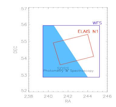
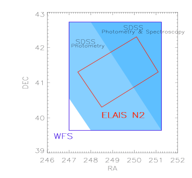
Figure 1: Coverage of the ELAIS N1 and N2 fields (small inner rectangles) by the WFS and the SDSS DR1 photometric and spectroscopic data.

Finally, as a part of the extensive program of ground based spectroscopy associated with the ELAIS survey, there have been follow-up observations of ELAIS 15 µm sources in the N1 and N2 fields (Pérez-Fournon et al. in preparation) using the WYFFOS multi-fibre spectrograph, on the William Herschel Telescope (WHT) at La Palma. This observing run added nine previously unknown quasars to the spectroscopic sample in the regions of N1 and N2 not covered by the spectroscopic DR1.

Therefore, a total of 25 spectroscopically confirmed quasars have been identified among the final ELAIS 15 µm catalogue and their properties are described in Table 1. Fig. 2 shows the 15 µm flux versus $r$-band flux for the quasar sample.

Table 1: ELAIS 15 µm spectroscopically confirmed quasars. $r$-band magnitude in column 5 is the SDSS $r$-band magnitude apart from the objects marked with an asterisk. These objects are outside the spectroscopic coverage of DR1 and the magnitude shown is the WFS $r$ magnitude. The last column (reference) refers to the origin of the spectra (1: Abazajian et al. 2003; 2: Pérez-Fournon et al. in preparation)

ELAIS ID	RA (optical)	Dec (optical)	z	$r$ mag	15 µm   flux (mJy)	$z$ Reference
ELAISC15_J160250.9+545057	240.71234131	54.84947205	1.1971	19.22	2.1820	SDSS1
ELAISC15_J160522.9+545613	241.34640503	54.93708420	0.5722	18.94	2.2160	SDSS1
ELAISC15_J160623.5+540556	241.59822083	54.09888840	0.8766	17.62	4.2930	SDSS1
ELAISC15_J160630.5+542007	241.62754822	54.33544159	0.8205	18.73	3.4460	SDSS1
ELAISC15_J160638.0+535009	241.65779114	53.83572006	2.9426	19.77	1.6010	SDSS1
ELAISC15_J161007.2+535814	242.52960205	53.97055435	2.0317	18.86	1.7400	SDSS1
ELAISC15_J163702.2+413022	249.25930786	41.50616837	1.1783	19.11	2.0920	SDSS1
ELAISC15_J163709.2+414031	249.28890991	41.67519760	0.7602	17.20	8.4090	SDSS1
ELAISC15_J163739.3+414348	249.41436768	41.72999954	1.4136	18.94	1.0610	SDSS1
ELAISC15_J163847.5+421141	249.69760132	42.19494629	1.7786	18.93	1.7420	SDSS1
ELAISC15_J163915.9+412834	249.81591797	41.47602844	0.6919	19.05	3.3730	SDSS1
ELAISC15_J163930.8+410013	249.87844849	41.00380707	1.0515	18.23	1.2580	SDSS1
ELAISC15_J163952.9+410346	249.97023010	41.06244278	1.6050	18.58	2.0940	SDSS1
ELAISC15_J164010.1+410521	250.04225159	41.08955383	1.0990	17.01	9.5570	SDSS1
ELAISC15_J164016.0+412102	250.06701660	41.35038757	1.7570	18.44	2.0900	SDSS1
ELAISC15_J164018.4+405812	250.07641602	40.97030640	1.3175	18.13	3.7700	SDSS1
ELAISC15_J161521.8+543148	243.84077454	54.53016663	0.4737	18.24*	3.492	WYFFOS2
ELAISC15_J161526.7+543004	243.86094666	54.50175095	1.3670	19.35*	1.457	WYFFOS2
ELAISC15_J161543.5+544828	243.93133545	54.80799866	1.6920	18.22*	2.107	WYFFOS2
ELAISC15_J163425.2+404152	248.60472107	40.69794464	1.6840	18.37	3.1690	WYFFOS2
ELAISC15_J163502.7+412953	248.76176453	41.49808502	0.4727	18.08	2.1730	WYFFOS2
ELAISC15_J163531.1+410025	248.87956238	41.00761032	1.1500	18.81	1.3990	WYFFOS2
ELAISC15_J163533.9+404025	248.89176941	40.67380524	0.5340	19.72	2.7300	WYFFOS2
ELAISC15_J163553.5+412054	248.97354126	41.34883118	1.1950	19.39	2.7260	WYFFOS2
ELAISC15_J163634.4+412742	249.14343262	41.46200180	0.1711	18.50	4.1540	WYFFOS2

Figure 2: $r$-band versus the 15 µm flux for the quasar sample. Filled (open) circles represent objects with SDSS (WYFFOS) spectra. Symbol size decreases with increasing redshift.

3 Variability

Variations in the luminosity of quasars have been observed from X-ray to radio wavelengths, with timescales of minutes to years. The majority of QSOs have continuum variability on the order of 10% on timescales of months to years (Vanden Berk et al., 2003). Furthermore, recent observations of radio-quiet quasars indicate that more than 80% show long-term (month to year) variability with amplitudes up to half a magnitude (Huber et al., 2002). Variability is wavelength dependent. The continuum ($F_{\nu}\propto\nu^{-\alpha}$) tends to get harder (the spectral index, $\alpha$, decreases) as the quasar gets brighter, which means that the variations are larger at shorter wavelengths.

The SDSS imaging strategy consists in observing in almost simultaneous mode the same field in the five different bands. The imaging strategy of the WFS was, however, different, and the same fields were observed in the different filters in timescales ranging from a few months to more than a year. Fig. 3 shows the differences of the magnitudes for the point sources lying in the common area in the two photometric systems. The magnitude differences show very small dispersions down to a certain magnitude for almost all point sources that are identified as stars but large variations appear in the case of many of the confirmed quasars (red crosses) in all filters but especially in the $U$- and $g$-bands, indicating variability related issues.

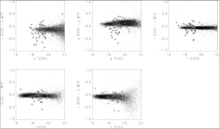
Figure 3: Magnitudes differences between SDSS and WFS, the black points represent the point sources, mostly stars, while the red crosses indicate the 73 confirmed quasars. The photometric errors for the quasars are lower than 0.05 magnitudes in all bands and the dispersion in their magnitudes is evident.

It might be argued that the variations are due to the different photometric systems, however close they may be. For this purpose, a simulated quasar catalogue was created, based on the colours of the SDSS composite quasar spectrum (Vanden Berk et al., 2001), including all 10 filters and for redshifts spanning from 0 to 6 and the magnitudes were compared. Fig. 4 illustrates the expected magnitude differences as a function of magnitude for redshifts in the interval [0,4], where all our spectroscopically confirmed quasars lie, and for the filters $U$, $g$ and $z$. Filters $r$ and $i$ were omitted for clarity as the points largely overlap with the rest of the points. Even though magnitude variations are predicted, their amplitude is significantly smaller than the ones observed. We therefore conclude that not all observed variations between the SDSS and WFS photometry can be explained by the differences of the photometric systems and that some must be a result of quasar variability.

Figure 4: Theoretical magnitude differences for the filters U, g, and z of the SDSS and WFS photometric systems, in the redshift interval [0,4]. Filters $r$ and $i$ have been omitted for clarity.

This strongly suggests that quasar candidates selection and photometric redshift estimates are likely not to be accurate for all objects when WFS or other similar data are used and additional methods have to be looked for.

4 QUASAR CANDIDATES SELECTION

For the purpose of identifying high probability quasar candidates from the available datasets we used two techniques, a combination of colour-colour diagrams (hereafter method 1 - M1) and the template fitting method (M2). M1, based on Richards et al. (2002), consists of a colour-colour selection algorithm trained using the SDSS Early Data Release (Stoughton et al., 2002), for low- to intermediate redshift ($\sim 2.5$) objects. M2 is the standard template fitting that simultaneously provides a photometric redshift estimate for the quasar candidates. The point source template library comprises quasar and stellar templates and the observed SED of each object is compared to the one computed by convolving each template with the filters transmissions (for further details see Hatziminaoglou et al. 2000 and 2002). M1 is expected to give higher confirmation rates (i.e. number of real quasars over then number of quasar candidates) at low and intermediate redshifts but its efficiency greatly depends on the photometric system used and can not be applied as such when other filters are used. M2 is subject to higher contamination from sources other than quasars (e.g. stars) but is expected to have a much better efficiency at high redshift and can be used for any filter combination. In order to improve the results, we also make use of the IR information available for the 15 µm sources keeping in mind that the combination of all these techniques will be applied in the near future in the framework of SWIRE.

A first test is made using the more reliable SDSS photometry (Section 4.1) but an attempt of selecting candidates based on the WFS photometry will also be presented (Section 4.2). Our test sample consists of 21 spectroscopically confirmed quasars with available SDSS photometry and 25 with WFS photometry, which include all 21 from SDSS (see Table 1). Fine-tuning the method for WFS data is very important as large part of the SWIRE fields have been observed by the WFS.

4.1 Quasar Candidates with SDSS Photometry

A sample of 82 15 µm ELAIS sources identified as point sources from their optical photometry (SDSS OBJC_TYPE = 6) with $r$-band magnitudes brighter that 22.6 has been selected from the SDSS photometric catalogue. The optical magnitude cut has been imposed in order to avoid spurious detections and large photometric errors.

Table 2: Comparison of the completeness and confirmation rate yielded by M1 and M2 on a sample of 82 SDSS point sources with 15 µm emission. The second column shows the number of quasar candidates ($N_{c}$) and the number of spectroscopically confirmed quasars among them ($N_{f}$).

Method	$N_{c}$ ($N_{f}$)	Completeness	Conf. Rate
M1	26 (19)	90%	73%
M2	33 (19)	90%	58%
M2 & C1	30 (19)	90%	63%

The 15 µm information can be used in order to impose IR conditions in the selection of quasar candidates. Stars, galaxies, and AGN all have different optical to mid-IR slopes, with stars typically having larger optical than mid-IR fluxes (González-Solares et al., 2004). Furthermore, according to models of galaxies in the IR (Rowan-Robinson, 2001), quasar mid-IR fluxes are some 10 to 100 times larger than their optical ones. Taking this into account, one can impose additional constraints on the selection criteria requiring a mid-IR to optical flux ratio of at least 10 for quasar candidates (hereafter condition C1). This condition allows the removal of three quasar candidates selected by $M2$ that have mid-IR to optical fluxes those of stars. Fig. 5 illustrates the positions of the different objects types and the regions where quasars and quasar candidates selected by the two methods lie.

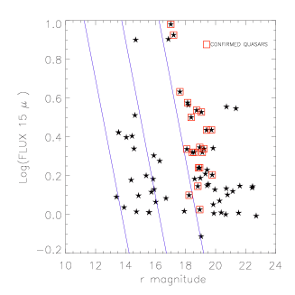
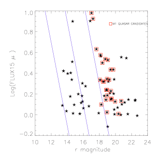
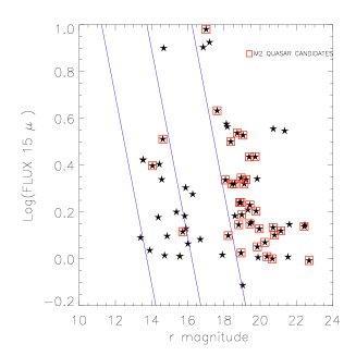
Figure 5: 15 µm flux (mJy) vs SDSS $r$-band magnitude for the point sources (stars) within the parts of ELAIS N1 and N2 areas covered by SDSS. The red squares indicate the confirmed quasars (left panel), M1 quasar candidates (central panel) and M2 quasar candidates (right panel). The blue lines represents constant 15 µm to $r$-band flux, with values 0.1, 1., and 10.

In order to distinguish between quasars and galaxies, one can make a combined use of optical and optical/IR colours taking advantage of the fact that quasars up to a redshift of $\sim 3$ are typically bluer than galaxies (González-Solares et al., 2004). Furthermore, 97.55% of all spectroscopically confirmed quasars in the DR1 quasar catalogue (Schneider et al., 2003) have $r-i<0.52$ (hereafter C2). Fig. 6 shows the distribution of stars (lower mid-IR to optical fluxes), galaxies and quasars (bluer than galaxies in general). Marked in red are the spectroscopically confirmed quasars (left panel) and the candidates selected by methods M1 and M2 (middle and right panels, respectively). As can be seen, all spectroscopically confirmed quasars form a clump bluewards of $r-i\sim 0.52$. In this particular case, C2 does not improve the results of any of the methods but will be used further on.

If $N_{c}$ is the number of quasar candidates stemming from the identification technique, $N_{f}$ the number of real quasars among the candidates, and $N_{e}$ the number of expected (based on models) or known (based on complete observations) quasars, completeness and confirmation rate can be defined as ${N_{f}}$/${N_{e}}$ and ${N_{f}}$/${N_{c}}$, respectively (Hatziminaoglou et al., 2000). Table 2 compares the two quantities yielded by the two methods. Both methods give the same completeness but the colour-colour selection favours the confirmation rate. Note, however, that the values given here for confirmation rate are lower limits. A substantial number of candidates (some 30%) are fainter than the SDSS spectroscopic completeness limit or lie outside the area covered by spectroscopy and therefore their nature is unknown. For the same reason, the value of the completeness is also indicative as a complete spectroscopic coverage would alter both $N_{f}$ and ${N_{e}}$.

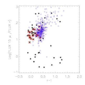
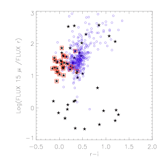
Figure 6: 15 µm to $r$-band flux vs SDSS $r-i$ for the point sources (stars) and extended sources (open circles). Red squares indicate spectroscopically confirmed quasars (left panel), M1 quasar candidates (central panel) and M2 quasar candidates (right panel).

4.2 Quasar Candidates with WFS Photometry

From the objects morphologically identified as point sources (SExtractor CLASS_STAR $\geq 0.9$) with detections at 15 µm 110 objects are part of the ELAIS Final Band-merged Catalogue (Rowan-Robinson et al., 2004). M1 yields 27 quasar candidates with 18 spectroscopically confirmed, while M2 finds 63 candidates with 25 spectroscopically confirmed (Table 1). The two candidate lists have 27 objects in common, 18 of which are spectroscopically confirmed quasars. Taking into account condition C1, 7 out of the 63 candidates proposed by M2 can be safely discarded as stars. Applying C2 on the remaining 56 candidates, we discard another five as more likely to be galaxies. Fig. 7 shows the positions of confirmed quasars and candidates, similar to Fig. 6, but for the WFS photometry.

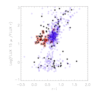
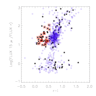
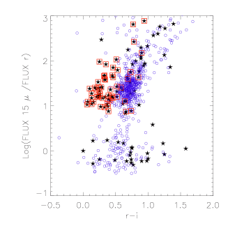
Figure 7: 15 µm to $r$-band flux vs WFS $r-i$ for the point sources (stars) and extended sources (open circles). In red squares, the spectroscopically confirmed quasars (left), M1 quasar candidates (centre) and M2 quasar candidates (right).

The results obtained using WFS photometry are summarised in Table 3. As already mentioned, the values of completeness are underestimated due to lack of complete spectroscopic coverage.

Table 3: Comparison of the completeness and confirmation rate yielded by M1 and M2 on a sample of 110 WFS point sources with 15 µm emission. The second column shows the number of quasar candidates ($N_{c}$) and the number of spectroscopically confirmed quasars among them ($N_{f}$).

Method	$N_{c}$ ($N_{f}$)	Completeness	Conf. Rate
M1	27 (18)	72%	67%
M2	63 (25)	100%	42%
M2 & C1	56 (25)	100%	45%
M2 & C1 & C2	51 (25)	100%	49%

After thorough consideration we reach the conclusion that WFS data can be used in order to reliably obtain quasar candidates despite the issues raised by variability, especially if one combines M1 and M2 with the constraints imposed by the objects’ IR properties.

4.3 Quasar Photometric Redshifts

For estimating the photometric redshifts we applied a standard template fitting procedure using synthetic quasar spectra consisting of a power law continuum and emission lines of fixed equivalent width values (Hatziminaoglou et al., 2000), on the sample of 73 spectroscopically confirmed quasars with both SDSS and WFS photometry available. The results are rather reliable when using SDSS photometry (53 out of 73 $\Delta z\leq$ 0.2, i.e. 73% ), but get worse when using the WFS photometry (29 out of 73 for $\Delta z\leq$ 0.2, i.e. 30% ). Note, however, that all seven objects with spectroscopic redshifts lower than 0.3 have been assigned the wrong photometric redshifts. These objects, however, are extended (OBJC_TYPE = 3) and, therefore, their magnitudes (psf magnitudes for SDSS and core magnitudes for WFS) must be contaminated by the light of the host galaxy. If we consider only the objects with spectroscopic redshifts higher than 0.3, the numbers of good identifications become 80% and 44%, for SDSS and WFS, respectively. Furthermore, all 30 objects that were assigned correct photometric redshifts using the WFS photometry have also correct photometric redshifts when SDSS photometry is used. Fig. 8 illustrates the results obtained for SDSS (left panel) and WFS (right panel) photometry.

Figure 8: Photometric versus spectroscopic redshifts for the 73 SDSS quasars within the ELAIS N1 and N2 areas, using SDSS (left) and WFS (right) photometry. The larger scatter in the right plot is most likely due to quasar variability, see text for details.

The fact that the bands for WFS photometry were taken in different periods of time (especially the $U$-band, which was taken more than two years apart in some cases) lead us to the conclusion that variability might be the basis of the discrepancy problem we encountered, as described in Section 3.

A case-by-case study of all objects that have correct photometric redshift estimates with SDSS photometry and bad estimates ($\Delta z>0.25$) with WFS photometry showed that they all lie in the redshift range [0.3,2.0] and their differences in magnitudes span a much larger range than the one expected due to the filters’ differences. One finally concludes that the wrong photometric redshift assignments are most probably due to variability, as argued earlier.

5 COMPARISON BETWEEN IR DETECTED AND NON-DETECTED QUASARS

36 spectroscopically confirmed quasars lie in the parts of the ELAIS N1 and N2 fields covered by the SDSS spectroscopic data release, with 16 of them detected at 15 µm, as already mentioned. Considering the homogeneous way the SDSS quasar candidates are selected (Richards et al., 2002) we can ask is if the two subsamples (16 IR and 20 non-IR emitters) have the same properties or if the IR detected quasars are, in some way, different. The colour-redshift (Fig.9) and colour-colour (Fig.10) diagrams of the two subsamples do not show any differences.

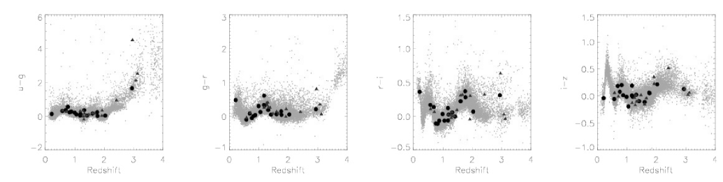
Figure 9: Colour - redshift diagrams for SDSS DR1 quasars (dots), non-ELAIS quasars (triangles) and ELAIS quasar (filled circles).

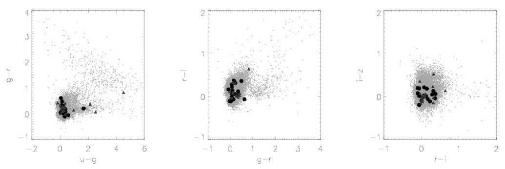
Figure 10: Colour - colour diagrams for SDSS DR1 quasars (dots), non-ELAIS quasars (triangles) and ELAIS quasar (filled circles).

A two-sided Kolmogorov-Smirnov test on the BH mass distributions of the two subsamples (seen in the right panel of Fig. 11) resulted in a larger than 90% probability for them to come from the same population. The same test gave a 35% probability for the redshift distributions to be representative of from the same population. The largest deviation is noticed in the $r$-band magnitude distributions (left panel of Fig. 11). The objects not detected by ISO at 15 µm are on average half a magnitude fainter in the $r$-band. Fig. 2 indicates a possible correlation between the 15 µm fluxes of the SDSS quasars and their optical ($r$-band) fluxes, suggesting that the lack of 15 µm counterparts could be due to their fainter magnitudes. Deeper IR observation would, presumably, provide counterparts for the remaining objects, since for a given covering fraction and varying bolometric luminosity, brighter optical AGN should have a higher mid-IR emission.

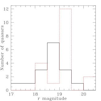
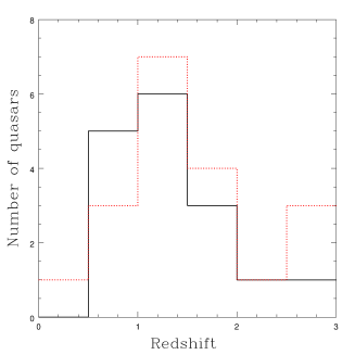
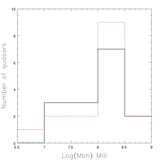
Figure 11: Histograms of $r$-band magnitude (left panel), redshift (middle panel) and black hole mass (right panel) for the ELAIS (black solid line) and non-ELAIS (red dotted line) quasars.

5.1 Quasar Black Hole Masses

The principal assumption underlying the BH virial mass estimate is that the dynamics of the Broad Line Region (BLR) are dominated by the gravity of the central supermassive black hole. Under this assumption an estimate of the central BH mass, $M_{BH}$, can be $M_{BH}\simeq R_{BLR}V^{2}/G$; where $R_{BLR}$ is the radius of the BLR and $V$ is the velocity of the line-emitting gas, traditionally estimated from the FWHM of the $H\beta$ emission line (see Kaspi et al. 2000). For quasars with redshifts higher than typically $z\sim 0.8$, when $H\beta$ is no longer available, McLure & Jarvis (2002) suggested the use of $MgII$ as an estimator of the BH mass. More precisely, the BH mass is computed as follows (McLure & Dunlop, 2004):

$$\frac{M_{bh}}{M_{\odot}}=4.7\left(\frac{\lambda L_{5100}}{10^{37}W}\right)^{0.61}\left(\frac{FWHM(H_{\beta})}{km/sec}\right)^{2}$$ (1)

and

$$\frac{M_{bh}}{M_{\odot}}=3.2\left(\frac{\lambda L_{3000}}{10^{37}W}\right)^{0.62}\left(\frac{FWHM(MgII)}{km/sec}\right)^{2}$$ (2)

For the sample of 36 SDSS quasars in N1 and N2, therefore, low redshift (up to $\sim 0.8$) mass estimates are based on the correlation between the $H\beta$ and the monochromatic luminosity at 5100 Å  (Eq. 1) while for higher redshift ones the correlation between $MgII$ and 3000 Å  luminosity (Eq. 2) is used. For objects with redshifts higher than 2, all estimators fall outside the covered wavelength range and BH masses can no longer be computed. Only objects with SDSS spectra were used for the BH mass computation as line and continuum of all SDSS spectra are measured in a consistent way by the SDSS pipeline.

Fig. 12 shows the distribution of BH mass as a function of redshift. Red marks the objects for which $H\beta$ was used (with redshifts typically lower than $\sim 0.8$), while black illustrates the ones for which $MgII$ was considered. Filled circles denote the objects with 15 µm emission while triangles correspond to SDSS objects within the ELAIS fields but without IR detections. BH masses show no differences between the two subsamples and follow the distributions found for the entire SDSS DR1 quasar catalogue by McLure & Dunlop (2004). The right panel of Fig. 11 shows the BH mass histogram for the two subsamples, clearly indicating that both of them belong to the same parent population.

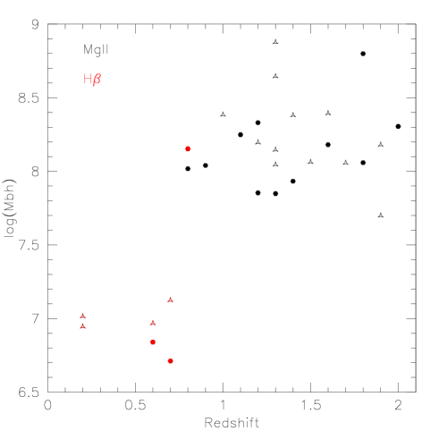
Figure 12: Black hole mass as a function of redshift for the ELAIS quasars with SDSS spectra (filled circles) and for the SDSS quasars without ELAIS counterparts (triangles).

For the objects for which the 15 µm fluxes were available, their IR luminosity was computed assuming an ($\Omega$, $\Lambda$) = (0.3, 0.7) cosmology. Fig. 13 shows the 15 µm IR luminosity of these objects as a function of redshift (left panel) and as a function of the BH mass (right panel). Clearly, high-mass BH tend to produce higher IR luminosities. Furthermore, the IR luminosity versus redshift distribution compares nicely to the findings of Pozzi et al. (2003), indicating that type I AGN in the redshift range [1,2] have IR luminosities higher than 10${}^{12}L_{\odot}$ (see Fig. 6 of Pozzi et al. 2003), proving thus that ISO only skimmed the brighter end of the luminosity function.

Figure 13: 15 µm IR luminosity of these objects as a function of redshift (left panel) and as a function of the BH mass (right panel).

6 DISCUSSION

This paper discusses some properties of the ELAIS 15 µm quasars and tries to establish a robust method of quasar selection for future use within the SWIRE framework. The importance of good quality ground-based data is stressed, both for the candidates selection and for the photometric redshifts estimates. Colour-colour plots and template fitting are used for these purposes. Colour-colour plots give a higher confirmation rate, as expected since they were trained on the same photometric system, while template fitting has the advantage of being independent of the filters used. The SDSS data have proved to be a reliable dataset, while the WFS data are somewhat less efficient due to the large timescales over which the imaging has been carried out and the variability issues this introduced. In order to correct for these effects, the IR and optical to IR properties of the objects have been taken into account imposing additional constraints on the quasar candidate selection techniques. The two subsamples of spectroscopically confirmed quasars detected and non-detected at 15 µm have been examined and they have shown no intrinsic physical differences. Their non-detection is most probably due to their fainter magnitudes, probably correlated to their higher redshifts.

This work can be seen as a validation of the tools and methods that will be used in the framework of SWIRE or other similar IR surveys supported by ground-based optical data. SWIRE will survey six high-latitude fields (including ELAIS N1 and N2), totaling 50 square degrees in all seven Spitzer bands. One of the key scientific goals of SWIRE is to determine the evolution of quasars in the redshift range 0.5$\leq z\leq$3 (Lonsdale et al., 2004). As we suggested in Section 5, with deeper IR observations one could detect all the quasars in the discussed fields down to the optical magnitude limit. In particular, the SWIRE 5$\sigma$ photometric sensitivity is 0.0037 mJy in the IRAC 8 µm band and 0.15 mJy in the MIPS 24 µm band, much deeper than the characteristic depth of $\sim 1$ mJy of ELAIS 15 µm (Vaccari et al., 2004). Last but not least, the multitude of the SWIRE bands will allow for a much better galaxy-AGN separation in the mid-IR colour space, possibly making the optical morphological preselection of quasar candidates obsolete.

Models (e.g. Granato & Danese 1994; Nenkova et al. 2002) and observations (e.g. Elvis et al. 1994) suggest that quasar IR spectra are more or less flat (in $\nu L_{\nu}$) from $\sim 1$ µm down to at least 25 µm, even in the absence of starburst activity. Therefore, the deeper and better quality SWIRE 8 µm and 24 µm observations will allow the detection of high numbers of quasars and the easy adaptation of the tools presented here. The stellar contamination will probably be higher at 8 µm than at 15 µm but this problem will most likely be solved due to the multitude of IR bands, that will allow an easier separation of the galactic and extragalactic populations.

As a last remark, we would like to stress that a robust candidate selection technique and subsequent photometric redshift estimates such as the ones presented here will be increasingly required by all future large area surveys, as spectroscopic coverage will never reach the same completeness, neither in area nor in depth.

ACKNOWLEDGMENTS

This paper is based on observations with ISO, an ESA project, with instruments funded by ESA Member States and with participation of ISAS and NASA. This work made use of data products provided by the CASU INT Wide Field Survey and the Sloan Digital Sky Survey. The INT and WHT telescopes are operated on the island of La Palma by the Isaac Newton Group in the Spanish Observatorio del Roque de los Muchachos of the Instituto de Astrofisica de Canarias. The SDSS Web site is http://www.sdss.org/. This work was supported in part by the Spanish Ministerio de Ciencia y Tecnologia (Grants Nr. PB1998-0409-C02-01 and ESP2002-03716) and by the EC network ”POE” (Grant Nr. HPRN-CT-2000-00138).

References

- Abazajian et al. (2003) Abazajian K., Adelman-McCarthy J., Agueros M.A., Allam S.A., Anderson S.F., Annis J., Bahcall N.A., Baldry I.K. et al., 2003, AJ, 126, 2081
- Cesarsky et al. (1996) Cesarsky C., Abergel A., Agnese P., Altieri B., Augueres J.L., Aussel H., Biviano A., Blommaert J., Bonnal J.F. et al., 1996, A&A, 315, 32L
- Elvis et al. (1994) Elvis M., Wilkes B.J., McDowell J.C., Green R.F., Bechtold J., Willner S.P., Oey M.S., Plomski E., Cutri R., 1994, ApJ, 95, 1
- Bolzonella et al. (2000) Bolzonella M., Miralles J.-M., Pelló R., 2000, A&A 363, 476-492
- Granato & Danese (1994) Granato G.L., Danese L., 1994, MNRAS, 268, 235
- González-Solares et al. (2004) González-Solares E.A., Pérez-Fournon I., Rowan-Robinson M., Oliver S., Vaccari M., Lari C., Irwin M., McMahon R.G. et al., 2004, MNRAS, submitted
- Hatziminaoglou et al. (2000) Hatziminaoglou E., Mathez G., Pelló R., 2000, A&A, 359, 9
- Hatziminaoglou et al. (2002) Hatziminaoglou E., Groenewegen M.A.T., da Costa L., Arnouts S., Benoist C., Madejsky R., Mignani R.P., Olsen L.F., Rite C. et al., 2002, A&A, 384, 81
- Huber et al. (2002) Huber M.E., Clowes R.G., Soechting I.K., Howell S.B., 2002, AAS, 201
- Kaspi et al. (2000) Kaspi S., Smith P.S., Netzer H., Maoz D., Jannuzi B.T., Giveon U., 2000, ApJ, 533, 631
- Kessler et al. (1996) Kessler M.F., Steinz J.A., Anderegg M.E., Clavel J., Drechsel G., Estaria P., Faelker J., Riedinger J.R., Robson A. et al., 1996, A&A, 315, 27L
- Lemke et al. (1996) Lemke D., Klaas U., Abolins J., Abraham P., Acosta-Pulido J., Bogun S., Castaneda H., Cornwall L., Drury L. et al., 1996, A&A, 315, 64L
- Lonsdale et al. (2003) Lonsdale C., Smith H.E., Rowan-Robinson M., Surace J., Shupe D., Xu C., Oliver S., Padgett D. et al., 2003, PASP, 115, 897
- Lonsdale et al. (2004) Lonsdale C., Polletta M., Surace J., Shupe D., Fang F., Xu K., Smith H.E., Siana B., Rowan-Robinson M. et al., 2004, ApJS, in press
- McLure & Jarvis (2002) McLure R., Jarvis M.J., 2002, MNRAS, 337, 109
- McLure & Dunlop (2004) McLure R., Dunlop J.S., 2004, MNRAS, in press
- McMahon et al. (2001) McMahon R.G., Walton N.A., Irwin M.J., Lewis J.R., Binclark P.S., Jones D.H., 2001, NewAR, 45, 97
- Nenkova et al. (2002) Nenkova M., Ivezic Z., Elitzur M., 2002, ApJ, 570, 9
- Oliver et al. (2000) Oliver S., Rowan-Robinson M., Alexander D.M., Almaini O., Balcells M., Baker A.C., Barcons X., Barden M. et al., 2000, MNRAS, 316, 749
- Peterson (1997) Peterson B.M., 1997, An Introduction to Active Galactic Nuclei, Cambridge University Press
- Pozzi et al. (2003) Pozzi F., Ciliegi P., Gruppioni C., Lari C., Heraudeau F., Mignoli M., Zamorani G., Calabrese E., Oliver S., Rowan-Robinson M., 2003, MNRAS, 343, 1348
- Richards et al. (2001) Richards G.T., Weinstein M.A., Schneider D.P. Fan X., Strauss M.A., Vanden Berk D.E., Annis J., Burles S. et al., 2001, AJ, 122, 1151
- Richards et al. (2002) Richards G.T., Fan X., Newberg H.J., Strauss M.A., Vanden Berk D.E., Schneider D.P. Yanny B., Boucher A. et al., 2002, AJ, 123, 2945
- Rowan-Robinson (2001) Rowan-Robinson M., 2001, NewAR, 45, 631
- Rowan-Robinson et al. (2004) Rowan-Robinson M., Lari C., Pérez-Fournon I., González-Solares E.A., La Franca F., Vaccari M., Oliver S., Gruppioni C. et al., 2004, MNRAS, 351, 1290
- Schneider et al. (2003) Schneider D.P., Fan X., Hall P.B., Jester S., Richards G.T., Stoughton C., Strauss M.A., SubbaRao M. et al., 2003, ApJ, 126, 2579
- Stoughton et al. (2002) Stoughton C., Lupton R.H., Bernardi M., Blanton M.R., Burles S., Castander F.J., Connolly A.J., Eisenstein D.J. et al, 2002, AJ, 123, 485
- Vaccari et al. (2004) Vaccari M., Lari C., Angeretti L., Fadda D., Gruppioni C., Pozzi F., Prouton O., Aussel H., Ciliegi P. et al., 2004, MNRAS, submitted, astro-ph/0404315
- Vanden Berk et al. (2001) Vanden Berk D.E.,Richards G.T., Bauer A., Strauss M.A., Schneider D.P., Heckman T.M., York D.G., Hall P.B. et al., 2001, ApJ, 122, 549
- Vanden Berk et al. (2003) Vanden Berk D.E., Wilhite B.C., Kron R.G., Anderson S.F., Brunner R,J., Hall P.B., Ivezic Z., Richards G.T. et al., 2004, ApJ, 601, 692