Abstract

The evolution of a nonaxisymmetric bar-mode perturbation of rapidly rotating stars due to a secular instability induced by gravitational wave emission is studied in post-Newtonian simulations taking into account gravitational radiation reaction. A polytropic equation of state with the polytropic index $n=1$ is adopted. The ratio of the rotational kinetic energy to the gravitational potential energy $T/|W|$ is chosen in the range between 0.2 and 0.26. Numerical simulations were performed until the perturbation grows to the nonlinear regime, and illustrate that the outcome after the secular instability sets in is an ellipsoidal star of a moderately large ellipticity $\mathrel{\raise 1.29167pt\hbox{$>$}\mkern-14.0mu\lower 2.58334pt\hbox{$\sim$}}0.7$. A rapidly rotating protoneutron star may form such an ellipsoid, which is a candidate for strong emitter of gravitational waves for ground-based laser interferometric detectors. A possibility that effects of magnetic fields neglected in this work may modify the growth of the secular instability is also mentioned.

I INTRODUCTION

Rapidly rotating stars are subject to nonaxisymmetric rotational instabilities. An exact treatment of these instabilities exists for incompressible and rigidly rotating equilibrium fluids in Newtonian gravity [1, 2]. For these configurations, global rotational instabilities arise from nonradial toroidal modes $e^{im\varphi}$ ($m=1,2,\dots$) when $\beta\equiv T/|W|$ exceeds a certain critical value. Here $\varphi$ is the azimuthal coordinate and $T$ and $W$ are the rotational kinetic and gravitational potential energies (see Sec. II B for definition). There exist two different types of mechanisms and corresponding time scales for the instabilities. One is the secular instability which, with a given value of $m$, sets in for a value of $\beta$ larger than a critical value $\beta_{s}$ and can grow in the presence of some dissipative mechanism, like viscosity or gravitational radiation. The growth time is determined by the dissipative time scale, which is usually longer than the dynamical time scale of the system. By contrast, a dynamical instability, which sets in for a value of $\beta$ larger than a critical value $\beta_{d}(>\beta_{s})$, is independent of any dissipative mechanisms, and the growth time is determined typically by the hydrodynamical time scale of the system. In this paper, we study the growth of a secularly unstable bar-mode for compressible stars whose growth is induced by the gravitational radiation. Hereafter, we only focus on the $m=2$ bar-mode since it is the fastest growing mode in most of rapidly rotating stars. (With regard to counter-examples in a narrow parameter range, see [3, 4] about secular instability.)

The criterion for the onset of the secular bar-mode instability for compressible rotating stars has been extensively determined by linear perturbative analyses in Newtonian theory [5, 6, 7, 8, 9, 10, 11, 12], in post-Newtonian approximation [13], and in general relativity [14, 15]. These studies indicate that the value of $\beta_{s}$ for a bar-mode is $\approx 0.14$ in many cases, although it varies depending on the rotational law, equations of state, and effect of general relativity. In particular, the value of $\beta_{s}$ could be decreased significantly below 0.14 for highly differentially rotating stars [12] and for a compact general relativistic star [14]. However, it is not increased much beyond 0.14 to our knowledge. Thus, in the presence of gravitational radiation reaction, the bar-mode perturbation can grow for rapidly rotating and secularly unstable stars with $\beta>0.14$.

The secular instability by gravitational wave emission may be relevant for rapidly and differentially rotating protoneutron stars formed soon after supernova collapse [4]. To study the growth of a secularly unstable bar-mode perturbation to a nonlinear perturbative regime, a longterm numerical simulation is necessary. However, such study has not been performed until quite recently even in the Newtonian or post-Newtonian gravity. (But, see [16] for a study of the incompressible case in which the basic equations reduce to ordinary differential equations, and [17] for a simulation of $r$ mode instability.)

There are several evolutionary paths which may lead to the formation of rapidly and differentially rotating neutron stars with $\beta>0.14$. Assuming mass and angular momentum conservation, $\beta$ increases approximately as $R^{-1}$ during stellar collapse where $R$ denotes the radius of the collapsing core. In rotating supernova collapse, the core contracts from $R\sim 2000$ km to a few 10 km (e.g., [18, 19, 20, 21] for Newtonian simulations and [23, 24] for general relativistic simulations), and hence, $\beta$ may increase by two orders of magnitude. In reality, a large fraction of the mass is ejected in the supernova explosion, and hence, the relation between $\beta$ and $R$ will not be as simple as expected (e.g., [23]). Nevertheless, the value of $\beta$ in the inner region that forms the protoneutron star should increase. The radius of a rotating progenitor star that forms a protoneutron star of radius $\sim 10$ km will be $\gg 100$ km, and hence, it is reasonable to expect that the value of $\beta$ will increase at least by one order of magnitude. Thus, a stellar core with the effective value of $\beta\mathrel{\raise 1.29167pt\hbox{$>$}\mkern-14.0mu\lower 2.58334pt\hbox{$\sim$}}10^{-2}$, which can be easily reached in differentially rotating cases [23], may yield rapidly rotating neutron stars which may reach the onset of secular or dynamical instability. Similar arguments hold for accretion induced collapse of white dwarfs to neutron stars [25] and for the merger of binary white dwarfs to neutron stars.

Only if the value of $\beta$ is in a range between $\beta_{s}$ and $\beta_{d}$, a rapidly rotating neutron star is secularly unstable but dynamically stable. Thus, it may be more likely that a rapidly rotating protoneutron star is dynamically unstable. The fate of dynamically unstable rotating stars against a bar-mode perturbation has been studied widely so far not only in Newtonian theory [26, 27, 28, 29, 30] but also in general relativity [31]. These studies have indicated that the value of $\beta_{d}$ is $\sim 0.27$ in many cases except for highly differentially rotating stars [30] and that after the growth of the bar-mode perturbation, spiral arms are formed, and then, angular momentum is transported outward with mass-shedding. As a result, the angular momentum of around the center of the rotating star is decreased below the dynamically unstable limit to be a slightly nonaxisymmetric star in which the value of $\beta$ is smaller than $\beta_{d}$. However, $\beta$ remains still much larger than $\beta_{s}$. Therefore, the relic of a dynamical instability can still be subject to a secular instability.

In this paper, we report the results of numerical simulations for the secular bar-mode instability of rapidly and differentially rotating protoneutron stars induced by gravitational radiation. The polytropic equation of state with the polytropic index $n=1$ is adopted to approximately model a protoneutron star. The hydrodynamic simulations are performed in a (0+2.5) post-Newtonian framework; i.e., Newtonian gravity and gravitational radiation reaction are taken into account [32]. While protoneutron stars are fairly compact objects with reasonably strong gravitational field, Newtonian theory is expected to describe them up to errors of the order $GM/Rc^{2}\sim 0.1$–0.2 where $G$, $c$, $M$, and $R$ are the gravitational constant, the speed of light, and mass and radius of the protoneutron stars, respectively.

Although a longterm, stable, and accurate numerical simulations are now feasible (e.g., [35]), a simulation for the growth of a nonaxisymmetric secular instability in full general relativity is still formidable because of the following reasons. (i) it is required to take a large computational region that is extended to a wave zone to correctly compute gravitational radiation reaction which is the key process in this issue, and (ii) it is required to perform a very longterm simulation because the growth time scale of a secularly unstable perturbation is much longer (several orders of magnitude longer) than the dynamical time scale of the system. These two facts imply that computational resources much larger than the present best ones are necessary to study this problem in fully general relativistic simulations. On the other hand, in a post-Newtonian simulation, (a) we can take into account the gravitational radiation reaction simply adding a radiation reaction potential, and hence, we do not have to take a large computational domain that is extended to a wave zone. Furthermore, (b) the magnitude of radiation reaction force can be artificially increased to shorten the radiation reaction time scale as short as a dynamical time scale. Specifically, we increase the magnitude of the radiation reaction term by a factor $\sim 10$–100 in this paper to accelerate the growth of a secularly unstable perturbation. (In the (0+2.5) post-Newtonian framework, increasing the radiation reaction force is equivalent to increasing the compactness of a star $GM/Rc^{2}$; see Sec. II A.) The facts (a) and (b) enable to reduce the computational time significantly, and hence, the study of the secular instability for compressible stars is feasible in a post-Newtonian framework with current computational resources.

The secular instability of rotating stars is also induced by viscous effects in a different way from that by gravitational radiation [1, 36, 4]: During the growth of the secular instability induced by gravitational radiation, vorticity is conserved but angular momentum is dissipated. On the other hand, in the case of viscosity, the angular momentum is conserved but the vorticity is dissipated. If the viscous dissipation time scale is as short as that of gravitational radiation, two effects interfere each other and suppress the growth of the secular instabilities [36]. An estimate suggests [4] that the viscous time scale in rapidly rotating protoneutron stars may not be as short as the dissipation time scale by gravitational waves, although it is not very clear. In this paper, we ignore the viscous effect as a first step and focus on the secular instability induced by gravitational radiation. Simulation adding the viscous term (solving the Navier-Stokes equations) is an interesting subject remained in the future.

The paper is organized as follows. In Sec. II, we describe basic equations, initial conditions, and the methods in numerical analysis. In Sec. III, the numerical results are presented paying attention to the growth time of a secularly unstable perturbation, the outcome after the growth of the secular instability, and gravitational waves. Section IV is devoted to a summary. Throughout this paper, we use the geometrical units of $G=c=1$.

II METHOD

A Basic equations

Numerical simulations are performed in a (0+2.5) post-Newtonian framework [32]. Here, “0” implies “Newtonian” order and “2.5” the lowest order radiation reaction effect due to mass-quadrupole gravitational wave emission. We adopt the following basic equations in Cartesian coordinates [32, 33, 34]:

$${\partial\rho\over\partial t}+{\partial\rho v^{j}\over\partial x^{j}}=0,$$ (1)

$${\partial\rho u_{i}\over\partial t}+{\partial(\rho u_{i}v^{j}+P\delta^{j}_{i})\over\partial x^{j}}=-\rho{\partial(\psi+\psi_{R})\over\partial x^{i}},$$ (2)

$${\partial\rho e\over\partial t}+{\partial(\rho e+P)v^{i}\over\partial x^{i}}=-h_{ij}v^{j}{\partial P\over\partial x^{i}}-\rho u_{i}{\partial(\psi+\psi_{R})\over\partial x^{i}}.$$ (3)

The first, second, and third equations are the continuity, Euler, and energy equations, respectively. Here, $\rho$, $P$, $e$, $v^{i}$, and $u_{i}$ are the baryon density, the pressure, the specific energy, the three velocity, and the spatial components of the four velocity. $e$ is the sum of the specific internal energy $\varepsilon$ and the specific kinetic energy as

$$e\equiv\varepsilon+{1\over 2}u_{i}u_{i}.$$ (4)

$v^{i}$ and $u_{i}$ are related by

$$u_{i}=\tilde{\gamma}_{ij}v^{j},$$ (5)

where $\tilde{\gamma}_{ij}=\delta_{ij}+h_{ij}$. For consistency, we compute $v^{j}$ by

$$v^{i}=\tilde{\gamma}^{ij}u_{j},$$ (6)

where $\tilde{\gamma}^{ij}$ is the inverse of $\tilde{\gamma}_{ij}$.

$\psi$, $\psi_{R}$, and $h_{ij}$ denote the Newtonian potential, the radiation reaction potential, and the tracefree tensor component of the radiation reaction metric. $\psi$ and $\psi_{R}$ are determined from the equations

$$\Delta\psi=4\pi\rho,$$ (7)

$$\psi_{R}\equiv{1\over 2}\biggl{(}-\Phi+h_{ij}x^{j}{\partial\psi\over\partial x^{i}}\biggr{)},$$ (8)

where $\Phi$ obeys

$$\Delta\Phi=4\pi h_{ij}x^{j}{\partial\rho\over\partial x^{i}}.$$ (9)

$h_{ij}$ can be related to the tracefree quadrupole moment $\hbox{$\,I\!\!\!\!-$}_{ij}$ as

$$h_{ij}=-{4G\over 5c^{5}}\epsilon{d^{3}\hbox{$\,I\!\!\!\!-$}_{ij}\over dt^{3}},$$ (10)

where

$$\hbox{$\,I\!\!\!\!-$}_{ij}\equiv\int d^{3}x\rho\biggl{(}x^{i}x^{j}-{1\over 3}r^{2}\delta^{ij}\biggr{)}.$$ (11)

In Eq. (10), we recover $c$ to clarify that it appears only in $h_{ij}$: In other terms of the basic equations, $c$ is not included explicitly. $\epsilon$ is introduced to control the strength of the radiation reaction force. Note that $\psi_{R}$ and $\Phi$ are also proportional to $\epsilon$. Hence, the radiation reaction time scale will be proportional to $\epsilon^{-1}$. To confirm that the growth time scale of the secular instability driven by gravitational radiation is indeed proportional to the inverse of $\epsilon$, we performed simulations varying the value of $\epsilon$.

The order of magnitude for $d^{3}\hbox{$\,I\!\!\!\!-$}_{ij}/dt^{3}$ for rapidly rotating stars is estimated as $\sim(GM/Rc^{2})^{5/2}$. Thus, $h_{ij}$ is totally proportional to $\epsilon(GM/Rc^{2})^{5/2}$. This implies that increasing the value of $\epsilon$ is equivalent to increasing the value of the compactness in the (0+2.5) post-Newtonian formalism. We note that the compactness in this framework does not have any meaning with regard to the strength of the self-gravity since in this framework, $c$ appears only in the terms associated with the gravitational radiation reaction. The compactness here is only the indicator for the magnitude of the radiation reaction force.

The third time derivatives of $\hbox{$\,I\!\!\!\!-$}_{ij}$ cannot be computed accurately by the straightforward finite-differencing since we adopt a second-order accurate finite-differencing in time. For the accurate computation, we adopt the same method as that adopted in previous papers (e.g., [37, 38]). In this method, the time derivatives of the quadrupole moment are rewritten appropriately operating the time derivatives in the integral and using the equations of motion. Then, the third time derivative of $\hbox{$\,I\!\!\!\!-$}_{ij}$ is written

$${d^{3}\hbox{$\,I\!\!\!\!-$}_{ij}\over dt^{3}}={\rm STF}\biggl{[}2\int d^{3}x\biggl{\{}2P{\partial v^{j}\over\partial x^{i}}-2\rho v^{i}{\partial\psi\over\partial x^{j}}+x^{i}{\partial\psi\over\partial x^{j}}{\partial\rho v^{k}\over\partial x^{k}}-\rho x^{i}{\partial(\partial_{t}\psi)\over\partial x^{j}}\biggr{\}}\biggr{]}+O(\epsilon),$$ (12)

where STF implies that the symmetric tracefree part should be extracted as

$${\rm STF}[T_{ij}]={T_{ij}+T_{ji}\over 2}-{\delta_{ij}\over 3}T_{kk},$$ (13)

and $T_{ij}$ is a tensor. The terms of order $\epsilon$ in $d^{3}\hbox{$\,I\!\!\!\!-$}_{ij}/dt^{3}$ yield the terms of order $\epsilon^{2}$ in $h_{ij}$, and thus, it is neglected.

During numerical simulation, we adopt the $\Gamma$-law equation of state

$$P=(\Gamma-1)\rho\varepsilon,$$ (14)

where $\Gamma$ is the adiabatic index, and in this paper, we set $\Gamma=2$ to model a moderately stiff equation of state for neutron stars as in [17]. With this equation of state, we can follow the formation of shocks that may form after the secular instability grows to a nonlinear regime.

The hydrodynamic equations are solved using a so-called high-resolution shock-capturing scheme we have recently adopted in fully general relativistic simulations [39, 35]. In this method, the transport terms in the hydrodynamic equations $\partial_{i}(\cdots)$ are computed by applying an approximate Riemann solver with third-order (piecewise parabolic) spatial interpolation. Detailed numerical methods with respect to the treatment of the transport terms (in the framework of general relativity) are described in [39]. The time integration is done with the second-order Runge-Kutta method. Atmosphere of small density ($\sim 10^{-6}$ of the central density $\rho_{c}$) outside stars is added for using the shock-capturing scheme. Since the hydrodynamic equations are written in the conservative form, the mass is conserved within the digit of double precision. The conservation of energy and angular momentum is slightly violated due to numerical dissipation besides the loss by gravitational waves.

In the (0+2.5) post-Newtonian formulation adopted here, we need to solve three Poisson equations for $\psi$, $\partial_{t}\psi$, and $\Phi$. They are solved by a preconditioned conjugate gradient method, for which the details are given in [38], with boundary conditions

$$\psi\rightarrow-{M\over r}-{3\over 2r^{3}}\hbox{$\,I\!\!\!\!-$}_{ij}n^{i}n^{j}+O(r^{-4}),$$ (15)

$$\partial_{t}\psi\rightarrow-{3\over 2r^{3}}{d\hbox{$\,I\!\!\!\!-$}_{ij}\over dt}n^{i}n^{j}+O(r^{-4}),$$ (16)

$$\Phi\rightarrow-{3\over 2r^{3}}C_{ij}n^{i}n^{j}+O(r^{-4}),$$ (17)

where $n^{i}$ is a radial unit vector $x^{i}/r$, $C_{ij}$ is a moment defined from the right-hand side of Eq. (9), and $M$ is the total baryon mass defined by

$$M=\int d^{3}x\rho.$$ (18)

We adopt a fixed uniform grid with size $141\times 141\times 141$ in $x-y-z$, which covers a region $-L\leq x\leq L$, $-L\leq y\leq L$, and $0\leq z\leq L$ where $L$ is a constant. We assume a reflection symmetry with respect to the equatorial plane, and set the grid spacing of $z$ to be half of that of $x$ and $y$. In all the simulations, the equatorial radius of rotating stars $R_{e}$ is set to be $5L/7$ (i.e., the equatorial radius is covered by 50 grid points). We also performed test simulations with size $113\times 113\times 113$ (i.e., the grid spacing becomes 1.25 times larger) for several selected cases and confirmed that the results depend weakly on the grid resolution. In the absence of radiation reaction, we checked the conservation of the total energy and angular momentum. The magnitude of the error monotonically increases with the number of time steps and for a typical simulation with $141\times 141\times 141$ grid size, after 30 central rotational periods ($P_{0}$), the violation of the total energy and angular momentum conservation is $\sim 5\%$ and $2\%$, respectively. We have checked that these values are decreased at approximately second order with improving the grid resolution. Even in the presence of gravitational radiation reaction, the vorticity should be conserved. We have monitored its conservation and found that for a region of relatively high density $\mathrel{\raise 1.29167pt\hbox{$>$}\mkern-14.0mu\lower 2.58334pt\hbox{$\sim$}}10^{-2}\rho_{c}$ where $\rho_{c}$ denotes the central density, it is conserved within $\sim 10\%$ error. (Around the surface of stars, the error is larger.) The violation of these conservation relations is due to numerical dissipation or diffusion.

Numerical simulations were performed on FACOM VPP5000 in the data processing center of National Astronomical Observatory of Japan. For one numerical simulation with size $141\times 141\times 141$, it takes about 8 CPU hours for 80,000 time steps using 48 processors.

B Initial conditions

A slightly perturbed rotating star is adopted as the initial condition for numerical simulation. Specifically, we first construct models of differentially rotating stars in axisymmetric equilibrium with values of $\beta=T/|W|$ past the secular instability threshold [12]. Here, in the notation of this paper, $T$ and $W$ are computed from

$$T\equiv{1\over 2}\int d^{3}x\rho\varpi^{2}\Omega^{2},$$ (19)

$$W\equiv{1\over 2}\int d^{3}x\rho\psi.$$ (20)

The equilibrium state is computed using the polytropic equation of state,

$$P=K\rho^{\Gamma},$$ (21)

where $K$ is the polytropic constant and $\Gamma=1+1/n$ with $n$ polytropic index. In this paper, we choose $\Gamma=2$ ($n=1$).

Since a realistic velocity profile for protoneutron stars is poorly known (e.g., [23]), we give a plausible one. As the angular velocity profile $\Omega(\varpi)$ where $\varpi=\sqrt{x^{2}+y^{2}}$, we choose the so-called $j$-constant-like law as

$$\Omega={\Omega_{0}A^{2}\over\varpi^{2}+A^{2}},$$ (22)

where $A$ is a constant, and $\Omega_{0}$ the angular velocity at the rotational axis ($z$ axis). The parameter $A$ controls the steepness of the angular velocity profile: For smaller values of $A$, the profile is steeper and for $A\rightarrow\infty$, the rigid rotation is recovered. In the present work, the value of $A$ is chosen to be equal to the equatorial radius $R_{e}$. In this case, the ratio of $\Omega_{0}$ to $\Omega$ at the equatorial surface is two, and hence, the star is moderately differentially rotating. Numerical simulations have shown that such a rapidly rotating star of moderate degree of differential rotation can be formed from initial conditions with rapid and moderately differential rotation [23]. As we have shown in previous papers [30], a star of a high degree of differential rotation, i.e., $\hat{A}\equiv A/R_{e}\mathrel{\raise 1.29167pt\hbox{$<$}\mkern-14.0mu\lower 2.58334pt\hbox{$\sim$}}0.5$ is dynamically unstable against nonaxisymmetric deformation even if it is not rapidly rotating with $\beta=O(0.01)$. However, with $\hat{A}=1$, the star is dynamically stable for $\beta\mathrel{\raise 1.29167pt\hbox{$<$}\mkern-14.0mu\lower 2.58334pt\hbox{$\sim$}}0.265$ [30, 40], and hence, the rapidly rotating stars with $0.2\leq\beta\leq 0.26$ that we adopt in this paper (cf. Table I) can be subject only to the secular instability. We also note that only for $\hat{A}\mathrel{\raise 1.29167pt\hbox{$<$}\mkern-14.0mu\lower 2.58334pt\hbox{$\sim$}}1$, a rotating star of a high value of $\beta\sim 0.25$ can be found for $\Gamma=2$ (e.g., [12]). Such a star which is secularly unstable but dynamically stable may be a plausible initial state of a rapidly rotating protoneutron star as mentioned in Sec. I. In addition, only for such a high value of $\beta$, the growth time scale of a secularly unstable mode is short enough to accurately follow the nonlinear growth of the perturbation.

In terms of $\beta$ and $\hat{A}$, one rotating star is determined for a given rotational profile and polytropic index. To specify a particular model, we could also specify the ratio of the polar radius $R_{p}$ to the equatorial radius $R_{e}$, i.e. $C_{a}=R_{p}/R_{e}$ instead of $\beta$. For the equations of state and the angular velocity profiles that we adopt in this paper, the value of $C_{a}$ monotonically decreases with increasing $\beta$ for any given set of $\hat{A}$ and $n$. This is the reason that $C_{a}$ can be a substitute for $\beta$.

We initially add a secularly unstable perturbation of a small amplitude on top of the equilibrium states. The density and velocity profiles of an unstable mode adopted are those computed by Karino and Eriguchi [12] in a linear perturbation analysis. In their analysis, the perturbed quantities are expanded as

$$\delta\rho=\sum_{m}\delta\rho_{m}(r,\theta)\cos(m\varphi-\sigma t),$$ (23)

$$\delta v^{r}=\sum_{m}\delta v^{r}_{m}(r,\theta)\sin(m\varphi-\sigma t),$$ (24)

$$\delta v^{\bar{\theta}}=\sum_{m}\delta v^{\bar{\theta}}_{m}(r,\theta)\sin(m\varphi-\sigma t),$$ (25)

$$\delta v^{\bar{\varphi}}=\sum_{m}\delta v^{\bar{\varphi}}_{m}(r,\theta)\cos(m\varphi-\sigma t),$$ (26)

where $\sigma$ is the angular velocity of the perturbation. The eigenfunctions are these found by solving the perturbed equations for $\delta\rho_{m}$ and $\delta v^{i}_{m}$ in the two dimensional space of $r$ and $\theta$. Here, $v^{\bar{\theta}}$ and $v^{\bar{\varphi}}$ denote the components associated with the orthonormal bases. We put an unstable mode of $m=2$ on a rotating equilibrium star at $t=0$. The profile of the perturbed quantities as well as the density and the rotational velocity on the equatorial plane are shown in Fig. 1 for $C_{a}=0.3$ for $m=2$, the only mode considered here. Note that the profile of the perturbed quantities is not as monotonic as that for rigidly rotating and incompressible stars [1]. Figure 1(b) displays density contour curves in $x$-$z$ plane for $C_{a}=0.3$ and shows that the rotating star is a flattened spheroid. In Table I, we also list several quantities of the perturbed rotating stars adopted as the initial condition. Here, the energy and the angular momentum are defined by

$$E\equiv\int d^{3}x\rho e+W,$$ (27)

$$J\equiv\int d^{3}x\rho u_{\varphi}.$$ (28)

(a)   (b)

FIG. 1.: (a) The profiles of the density, the rotational velocity, and the perturbed quantities on the equatorial plane, and (b) the density contour curves in $x$-$z$ plane for $C_{a}=0.3$. The density and the rotational velocity are normalized by $\rho_{c}$ and $\Omega_{0}R_{e}$, respectively. The amplitude of the perturbation is normalized so that the maximum value of $v^{r}$ is unity in units of $G=\rho_{c}=R_{e}=1$. Here, $v^{\bar{\varphi}}=\varpi v^{\varphi}$. The density contour curves are drawn for $\rho/\rho_{c}=0.1j$ for $j=0.01,0.1,1,2,\cdots,8,9,9.5$, and 10.

$R_{p}/R_{e}$	$T/|W|$	$M/(\rho_{c}R_{e}^{3})$	$E/(M^{2}/R_{e})$	$J/(M^{3/2}R_{e}^{1/2})$	$\Omega_{0}/\rho_{c}^{1/2}$	$\sigma/\Omega_{0}$	$\sigma_{+}/\Omega_{0}$	$I_{\varpi\varpi}/(MR_{e}^{2})$	$\hat{\epsilon}$	$\tau/P_{0}$	$\tau_{\rm anal}/P_{0}$
0.30	0.256	0.567	$-0.538$	0.366	1.34	0.569	0.914	0.288	0.25	3.5	5.9
0.334	0.237	0.557	$-0.546$	0.347	1.30	0.455	1.02	0.278	0.24	15	34
0.35	0.229	0.565	$-0.547$	0.339	1.29	0.419	1.06	0.275	0.25	31	60
0.40	0.203	0.610	$-0.547$	0.315	1.26	0.290	1.16	0.272	0.31	—	$510$

TABLE I.: Several quantities for secularly unstable rotating stars are shown in units of $G=R_{e}=\rho_{c}=1$ where $\rho_{c}$ is the central density at $t=0$. $\sigma$ is the angular velocity of the unstable mode and $\tau$ is the growth time scale of the secularly unstable mode found in numerical simulation for the value of $\hat{\epsilon}\equiv\epsilon(GM/R_{e}c^{2})^{5/2}$ given here in units of $P_{0}\equiv 2\pi/\Omega_{0}$ (the rotational period along the $z$ axis). Note that the value of $\hat{\epsilon}$ of a realistic neutron star with the equatorial radius 10–20 km and the mass $1.4M_{\odot}$ is 0.018–0.003. “—” implies that we could not determine the value of $\tau$ since it is too large. For all the models, the central density is normalized to be unity.

The growth time of a secularly unstable mode is approximately proportional to $\hat{\epsilon}^{-1}\equiv\epsilon^{-1}(GM/R_{e}c^{2})^{-5/2}$. Thus, to accelerate the growth, we artificially increased the value of $\hat{\epsilon}$ by a factor of 10–100. The values chosen in this work are listed in Table I. In the following, we will refer to the case listed in Table I as “$\epsilon=1$” case. To increase $\hat{\epsilon}$, we may either increase the value of $\epsilon$ or the value of compactness. As mentioned in Sec. II A, the compactness can be rather arbitrarily increased in the (0+2.5) post-Newtonian framework. In our choice of $\hat{\epsilon}$ for numerical computation, setting $\epsilon=1$ is equivalent to choosing very compact stars with $GM/R_{e}c^{2}\sim 0.6$, which is about 3–6 times as large as that of a neutron star or protoneutron star. We note that in general relativity, a star with $GM/R_{e}c^{2}\sim 0.6$ collapses to a black hole. However, in the (0+2.5) post-Newtonian theory, a star of any value of $GM/R_{e}c^{2}$ is stable against collapse for $\Gamma=2$. As a result, we can adopt such a large compactness of which the growth time scale of the secularly unstable mode is short enough to accurately follow its growth numerically. This is a great advantage in this post-Newtonian framework.

C Method for analysis

The growth of a nonaxisymmetric bar-mode perturbation is monitored using a distortion parameter defined as

$$\eta\equiv(\eta_{+}^{2}+\eta_{\times}^{2})^{1/2},$$ (29)

where

$$\eta_{+}\equiv{I_{xx}-I_{yy}\over I_{xx}+I_{yy}},$$ (30)

$$\eta_{\times}\equiv{2I_{xy}\over I_{xx}+I_{yy}},$$ (31)

and $I_{ij}~{}(i,j=x,y,z)$ denotes the quadrupole moment.

Throughout this paper, we choose initial conditions in which $\eta\sim 0.01$ or 0.05 at $t=0$ by appropriately multiplying a constant to $\delta\rho_{m}$ and $\delta v^{i}_{m}$. (Hereafter, we denote the initial value of $\eta$ as $\eta_{0}$.) When the instability grows, $\eta$ should increase in proportional to $e^{t/\tau}$ where $\tau$ denotes the growth time scale. Thus, we fit the time evolution of $\eta$ and determine the value of $\tau$.

During numerical simulation, gravitational waves are computed in the quadrupole formula [41] in which “$+$” and “$\times$” polarization modes of the waveforms are defined as

$$h_{+}\equiv{\ddot{I}_{xx}-\ddot{I}_{yy}\over r},~{}~{}~{}~{}h_{\times}\equiv{2\ddot{I}_{xy}\over r},$$ (32)

and the luminosity and the angular momentum flux by

$$L_{\rm GW}\equiv{1\over 5}\sum_{i,j}\hbox{$\,I\!\!\!\!-$}_{ij}^{(3)}\hbox{$\,I\!\!\!\!-$}_{ij}^{(3)},$$ (33)

$$\dot{J}_{\rm GW}\equiv{2\over 5}\sum_{j}(\hbox{$\,I\!\!\!\!-$}_{xj}^{(2)}\hbox{$\,I\!\!\!\!-$}_{yj}^{(3)}-\hbox{$\,I\!\!\!\!-$}_{yj}^{(2)}\hbox{$\,I\!\!\!\!-$}_{xj}^{(3)}),$$ (34)

where

$$\ddot{I}_{ij}={d^{2}I_{ij}\over dt^{2}},~{}~{}~{}~{}~{}\hbox{$\,I\!\!\!\!-$}_{ij}^{(n)}={d^{n}\hbox{$\,I\!\!\!\!-$}_{ij}\over dt^{n}}~{}~{}(n=2,3),$$ (35)

and $r$ is the distance from the source to a detector. $h_{+}$ and $h_{\times}$ presented here are the waveforms observed along the rotational ($z$-) axis. Thus, effectively, they represent the maximum amplitude.

III NUMERICAL RESULTS

A The growth of secularly unstable bar-mode perturbations

(a)    (b)

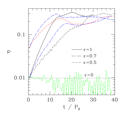
FIG. 2.: (a) $\eta$ as a function of time for $C_{a}=0.3$ (solid curve), 0.334 (dashed curve), and 0.35 (dotted-dashed curve) with $\epsilon=1$ and $\eta_{0}\sim 0.01$. For comparison, the results with $\eta_{0}\sim 0.04$ are shown for $C_{a}=0.334$ (long-dashed curve) and $C_{a}=0.35$ (dotted-long-dashed curve). The dotted curves denote the results with a low-resolution grid for $C_{a}=0.30$ and $C_{a}=0.334$ with $\eta_{0}\sim 0.04$. (b) $\eta$ as a function of time is shown for $C_{a}=0.3$ with $\epsilon=1$ (solid curve), 0.7 (long-dashed curve), 0.5 (dotted-dashed curve), and 0 (no radiation reaction; dotted-long-dashed curve). The dotted line denotes $\eta=\eta_{0}$. For $\epsilon=0.5$ and 0.7, results with $\eta_{0}\sim 0.05$ are shown together.

Numerical simulations were performed for secularly unstable stars with $C_{a}=0.3$, 0.334, 0.35, and 0.4. For the case with $C_{a}\mathrel{\raise 1.29167pt\hbox{$<$}\mkern-14.0mu\lower 2.58334pt\hbox{$\sim$}}0.52$ ($\beta\mathrel{\raise 1.29167pt\hbox{$>$}\mkern-14.0mu\lower 2.58334pt\hbox{$\sim$}}0.14$), the star of $\hat{A}=1$ and $\Gamma=2$ is secularly unstable according to the result of a linear perturbation analysis by Karino and Eriguchi [12]. In Fig. 2 (a), we show $\eta$ as a function of time for $C_{a}=0.3,0.334$, and 0.35 with $\epsilon=1$. For all cases, $\eta$ increases with time approximately as $e^{t/\tau}$. The plausible reason for a slight deviation from the exponential form is that modes other than the secularly unstable ones are excited due to numerical noise or nonlinear coupling, which contribute to the growth and modulation of $\eta$ soon after we start the simulation. However, they are not unstable modes, and hence, their amplitude does not increase. As a result, after the amplitude of the unstable mode increases for $t\mathrel{\raise 1.29167pt\hbox{$>$}\mkern-14.0mu\lower 2.58334pt\hbox{$\sim$}}2P_{0}$, the effect of other modes does not seem to be very large. From this reason, we determine the value of $\tau$ from the curve of $\eta$ for $t\mathrel{\raise 1.29167pt\hbox{$>$}\mkern-14.0mu\lower 2.58334pt\hbox{$\sim$}}2P_{0}$. More specifically, we use the data sets of $2P_{0}\leq t\leq 7P_{0}$ for $C_{a}=0.3$, of $2P_{0}\leq t\leq 20P_{0}$ for $C_{a}=0.334$ with $\eta_{0}\sim 0.04$, and of $2P_{0}\leq t\leq 30P_{0}$ for $C_{a}=0.35$ with $\eta_{0}\sim 0.04$. We expect that the error for the evaluation of $\tau$ is $\sim 10$% for $C_{a}=0.3$ and 0.334. For $C_{a}=0.35$, the growth time scale is too long to follow the late evolution with a sufficient accuracy. Moreover, a modulation in $\eta$ prevents the accurate evaluation of the growth time scale. Thus, the magnitude of the error in the numerical result of $\tau$ for $C_{a}=0.35$ may be $>10$%.

From the analysis, we determine $\tau/P_{0}\approx 3.5$, 15, and $31$ for $C_{a}=0.30$, 0.334, and 0.35 (see Table I). For $C_{a}=0.334$ and 0.35, the growth time is also evaluated from the data with $\eta_{0}\sim 0.01$, and we find that the results agree approximately with those for $\eta_{0}\sim 0.04$. This shows that the growth time is independent of the value of $\eta_{0}$.

According to a linear perturbative analysis for the bar-mode secular instability of incompressible and rigidly rotating stars, the growth time of the secularly unstable perturbation induced by emission of gravitational waves is [5]

$$\tau_{\rm anal}={5(\sigma_{+}-\sigma)\over 2I_{\varpi\varpi}\sigma^{5}},$$ (36)

where $\sigma$ is the angular velocity of the secularly unstable mode, $\sigma_{+}$ is that of its conjugate mode, which is a secularly stable one, and $I_{\varpi\varpi}\equiv I_{xx}+I_{yy}$. Equation (36) is valid only for the incompressible and rigidly rotating case. For $n\not=0$, it may be an approximate formula [4], but it is not very clear. Using the numerical results for $\sigma$ and $\sigma_{+}$ in a linear perturbative analysis by Karino and Eriguchi [12], the value of $\tau_{\rm anal}$ is evaluated and listed in Table I. It is found that the value of $\tau$ computed from the numerical results is systematically smaller than $\tau_{\rm anal}$: $\tau/\tau_{\rm anal}\sim 0.5$–0.6. The systematic disagreement will be due to the fact that Eq. (36) is valid only for the incompressible and rigidly rotating star. Indeed, the profile of the perturbed quantities is significantly different from that for incompressible and rigidly rotating stars [1]. On the other hand, the value of $\tau$ increases steeply as $\sigma/\Omega_{0}$ decreases by a similar manner to that described in Eq. (36). This indicates that the perturbation certainly grows due to the secular instability induced by gravitational radiation reaction.

To check that $\tau$ is proportional to $\epsilon^{-1}$, in Fig. 2 (b), we show $\eta$ as a function of time for $C_{a}=0.3$ with $\epsilon=1$ (solid curve), 0.7 (long-dashed curve), 0.5 (dotted-dashed curve), and 0 (no radiation reaction; dotted-long-dashed curve). In these simulations, the compactness $GM/R_{e}c^{2}$ is fixed. For $\epsilon=1$, $\eta_{0}\sim 0.01$, but for $\epsilon=0.7$ and 0.5, $\eta_{0}$ is set to be $\sim 0.01$ and 0.05. For the case with no radiation reaction, the value of $\eta$ does not increase but simply oscillates due to the growth of modes other than the secularly unstable one probably by numerical noises and nonlinear coupling. This shows that the star with $C_{a}=0.3$ is dynamically stable. (For $\hat{A}=1$ and $\Gamma=2$, only the stars with $C_{a}\mathrel{\raise 1.29167pt\hbox{$<$}\mkern-14.0mu\lower 2.58334pt\hbox{$\sim$}}0.25$ are dynamically unstable as demonstrated in [30].) The growth time $\tau$ is determined by the same method as that adopted above. The analysis gives $\tau/P_{0}=3.5$, 4.9, and 7.4 with an error of magnitude $\sim 10$% for $\epsilon=1$, 0.7, and 0.5. Thus, $\tau/P_{0}$ is approximately proportional to $\epsilon^{-1}$. We also note that $\tau$ also depends very weakly on the value of $\eta_{0}\mathrel{\raise 1.29167pt\hbox{$<$}\mkern-14.0mu\lower 2.58334pt\hbox{$\sim$}}0.05$. This implies that the amplitude of the nonaxisymmetric perturbation initially given is small enough.

Figure 2(b) also indicates that the value of $\eta$ eventually reaches $\sim 0.3$ and remains between $\sim 0.2$ and $\sim 0.3$. This shows that an ellipsoid is formed. The maximum value of $\eta$ (hereafter $\eta_{\rm max}$) at the formation of the ellipsoid depends weakly on the magnitude of the parameter $\epsilon$. However, the shape of the curve of $\eta(t)$ for $\eta\mathrel{\raise 1.29167pt\hbox{$>$}\mkern-14.0mu\lower 2.58334pt\hbox{$\sim$}}0.1$ is fairly different. For $\epsilon=1$, $\eta$ increases almost monotonically to the maximum value, but for $\epsilon=0.7$ and 0.5 with $\eta_{0}\sim 0.01$, the growth rate is varied at a time that $\eta$ becomes $\sim 0.1$. A plausible explanation for this difference is that the radiation reaction time scale is too short to obtain a qualitatively independent result of the value of $\epsilon$: We recall that the radiation reaction force adopted here has an invariant meaning only when the system is adiabatic, i.e., the system is nearly periodic and the reaction time scale is much longer than the period of a nonaxisymmetric oscillation. For $C_{a}=0.3$ with the compactness $\sim 0.6$, the reaction time scale is only a few times as long as the period of the nonaxisymmetric oscillation $\sim 2P_{0}\sim\tau\epsilon^{-1}/2$. This fact may be reflected in the difference of the shape of the curve of $\eta$.

In Fig. 2 (a), we display the results with a low-resolution grid for $C_{a}=0.3$ and $\eta_{0}\sim 0.01$ and for $C_{a}=0.334$ and $\eta_{0}\sim 0.04$ (dotted curves). For both cases, $\epsilon=1$. The growth time of $\eta$ and the maximum value of $\eta$ agree approximately with those for the high-resolution simulation. The growth time is slightly longer for the lower resolution simulations. This indicates that for a larger numerical dissipation, the growth time scale is spuriously increased. However, the grid resolution adopted here is high enough to obtain a convergent result.

B The fate of unstable stars

FIG. 3.: Snapshots of the density contour curves in the equatorial plane for $C_{a}=0.3$ and $\epsilon=1$. $\eta_{0}\approx 0.01$ in this case. The contour curves are drawn for $\rho/\rho_{c}=0.1j$ for $j=0.01,0.1,1,2,\cdots,8,9,9.5$, and 10. Vectors indicate the local velocity field $(v^{x},v^{y})$, and the scale is shown in the upper right-hand corner in units of $\rho_{c}^{1/2}R_{e}$. $P_{0}$ denotes the central rotational period of the equilibrium configuration given at $t=0$ ($P_{0}\approx 4.674$ in units of $G=R_{e}=\rho_{c}=1$).

FIG. 4.: The same as Fig. 3 but for $C_{a}=0.334$ and $\epsilon=1$. $\eta_{0}\approx 0.04$ in this case. $P_{0}\approx 4.826$ in units of $G=R_{e}=\rho_{c}=1$.

In Figs. 3 and 4, we display snapshots of the density contour curves and the velocity vectors in the equatorial plane for $C_{a}=0.3$, $\epsilon=1$, and $\eta_{0}\approx 0.01$, and for $C_{a}=0.334$, $\epsilon=1$, and $\eta_{0}\approx 0.04$. With the growth of a secularly unstable and nonaxisymmetric perturbation, the spheroidal shape is changed to an ellipsoidal shape, and after the value of $\eta$ reaches 0.1–0.3, the nonlinear growth of the perturbation terminates. Since the value of $\eta$ remains of order 0.1, the termination of the growth of the nonaxisymmetric deformation appears to happen when the rotating star reaches a quasistationary ellipsoidal state (see below for more discussion). Here, “quasistationary” implies that the axial ratio of the ellipsoid does not change in a dynamical time scale and the evolution is determined by the radiation reaction time scale which is much longer than the dynamical time scale of system.

The value of $\eta_{\rm max}$ does not depend strongly on the value of $\eta_{0}$ [cf. Fig. 2(a)], but it does on $C_{a}$. In particular, the smaller the value of $C_{a}$, the larger the value of $\eta_{\rm max}$ so that $\eta_{\rm max}\sim 0.3$, 0.2, and 0.1 for $C_{a}=0.3$, 0.334, and 0.35, respectively. This feature is expected from a study for the incompressible fluid [16] and as well as from a compressible ellipsoidal model [4]. As the maximum value of $\eta$ is reached, a semi major axial ratio of the formed ellipsoid defined in the equatorial plane also depends on the value of $C_{a}$. For $C_{a}=0.3$, the axial ratio of the ellipsoid $\approx\sqrt{(1-\eta)/(1+\eta)}$ reaches $\sim 0.75$, and the numerical results suggest that it is smaller for the larger value of $C_{a}$. We note that for an incompressible star [4], the axial ratio reached for $\beta\sim 0.25$ should be much smaller than 0.75. This may be a consequence that a rotating star with larger value of $n$ is less prone to forming an ellipsoid [42]. However, even for $\Gamma=2$, the axial ratio of the semi major axes is fairly large for $C_{a}\mathrel{\raise 1.29167pt\hbox{$<$}\mkern-14.0mu\lower 2.58334pt\hbox{$\sim$}}0.35$, and therefore, the ellipsoid will subsequently emit gravitational waves of large amplitude and dissipate energy and angular momentum due to a longterm emission of gravitational waves (cf. Sec. III C).

(a)   (b)

FIG. 5.: (a) The density and angular velocity profile along $x$ and $y$ axes at $t=0$ (dotted curves) and $t=12.8P_{0}$ (solid and dashed curves) for $C_{a}=0.3$ and $\epsilon=1$. The solid and dashed curves denote the profiles along $x$ and $y$ axes, respectively. (b) The same as (a) but for $C_{a}=0.334$ and $t=24.9P_{0}$.

In Fig. 5, we show the profiles of the density and angular velocity along the $x$ and $y$ axes at selected time slices. The contour curves and the velocity vectors at the corresponding time steps are shown in the third panels of Figs. 3 and 4. In other words, Figures 5(a) refers to the profile at $t/P_{0}=12.8$ for $C_{a}=0.3$ and $\epsilon=1$, and Fig. 5(b) is at $t/P_{0}=24.9$ for $C_{a}=0.334$ and $\epsilon=1$ with $\eta_{0}\approx 0.04$. In each figure, the density and the angular velocity at $t/P_{0}=0$ (dotted curves) are shown together. Around the origin, the density profile does not change significantly even after the formation of the ellipsoid. (Note that the central density decreases with time partly due to a numerical dissipation or diffusion.) However, around $\varpi/R_{e}\sim 0.5$–0.6, a density peak along the semi major axis is formed irrespective of the initial condition. Also, it is found that a nonaxisymmetry is enhanced around $\varpi/R_{e}>0.2$. These features found in the density profiles reflect the initial perturbation profile [cf. Fig. 1(a)]. After the formation of the ellipsoid, differential rotation is also enhanced as the result of the growth of the nonaxisymmetric density perturbation. It is interesting to note that a high-density and nonaxisymmetric peak rotates with a smaller rotational speed than that for the unperturbed axisymmetric star. This seems to be reasonable because the secularly unstable mode has an angular velocity smaller than the rotational angular velocity of the unperturbed equilibrium state.

In Fig. 6, the evolution of the total angular momentum $J$ and $\beta$ are shown for $C_{a}=0.3$, and $\epsilon=1$ (solid curve), 0.7 (long dashed curve), and 0 (dashed curve). Even for $\epsilon=0$ for which the system should be almost stationary throughout the simulation, $J$ increases by $\sim 2\%$ and $\beta$ decreases by $\sim 1\%$ in $30P_{0}$. These are the typical truncation error with grid of $141\times 141\times 141$. For $\epsilon>0$, during the exponential growth of the secularly unstable mode, $J$ and $\beta$ decrease at most 1% by gravitational wave emission. (Compare the curves with $\epsilon=0$ and $\epsilon\not=0$. The difference between two values can be regarded as loss by the gravitational radiation.) Thus, the formed ellipsoid initially has slightly smaller values of $J$ and $\beta$ than those of the secularly unstable axisymmetric star in equilibrium. After the formation of a quasistationary ellipsoid, these values start decreasing significantly due to dissipation by gravitational waves. Figure 6 indicates that when the ellipsoid relaxes to a final stationary state that does not emit gravitational waves, the values of $J$ and $\beta$ will be much smaller than the initial values.

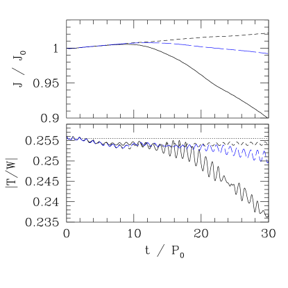
FIG. 6.: Evolution of $J$ and $\beta=T/|W|$ for $C_{a}=0.3$, and $\epsilon=1$ (solid curve), 0.7 (long dashed curve), and 0 (dashed curve). $J_{0}$ denotes the initial value of $J$.

The final state after a sufficient emission of gravitational waves is uncertain. For an incompressible fluid star, it will be a Dedekind ellipsoid which is static in shape and has only internal motion and no pattern rotation if it is observed in the inertial frame. However, for $n\mathrel{\raise 1.29167pt\hbox{$>$}\mkern-14.0mu\lower 2.58334pt\hbox{$\sim$}}0.8$, such configuration may not exist because of the following facts: (i) the uniformly rotating ellipsoid (Jacobi-like ellipsoid) does not exist for $n>0.808$ [42] and (ii) the Dedekind theorem for the incompressible fluid tells that the absence of the Jacobi ellipsoid implies the absence of the Dedekind ellipsoid [1]. Namely, if this theorem holds for $n\not=0$, no Dedekind-like configuration would exist for $n>0.808$. Lai and Shapiro expect that the final state may be a Dedekind-like ellipsoid even for $n>0.8$ [4]. The other possibility is that the unstable star does not relax to a Dedekind-like ellipsoid but to a (nearly) axisymmetric and secularly stable rotating star after sufficient emission of gravitational waves. The results of the present simulation indicate that the latter is more likely because of the following reasons.

For the incompressible case, a secularly unstable Maclaurin spheroid changes to a Dedekind ellipsoid by emission of gravitational waves conserving the vorticity [4]. Throughout this transition, the energy and the angular momentum are decreased at most by a few percents from their initial values [4]. Furthermore, for $\beta\sim 0.25$, the axial ratio in the equatorial plane becomes very small $\ll 0.75$. In the case of $C_{a}=0.3$, $\eta_{0}\sim 0.01$, and $\epsilon=1$, until the end of the simulation at $t\sim 30P_{0}$, the energy and the angular momentum are dissipated by gravitational waves by $\sim 5\%$ and $\sim 10\%$, respectively. However, even at $t\sim 30P_{0}$, the rotating stars still do not settle into a highly deformed Dedekind-like ellipsoid but to a moderately deformed quasistationary (Riemann-type) ellipsoid which emits gravitational waves of a moderately large amplitude (cf. Sec. III C). The results of the simulation also indicate that the gravitational wave emission does not enforce the ellipsoid to a stationary state immediately, although the final outcome should be an object that does not emit gravitational waves. Thus, the ellipsoid will subsequently emit gravitational waves for a long time to dissipate the energy and the angular momentum by $\mathrel{\raise 1.29167pt\hbox{$>$}\mkern-14.0mu\lower 2.58334pt\hbox{$\sim$}}10\%$. Indeed, Fig. 6 suggests that $\beta$ will decrease much below the initial value. Therefore, in the present case, the final state after a longterm dissipation by gravitational waves will not be a highly deformed Dedekind-like ellipsoid, but a nearly axisymmetric spheroid of $\beta\ll 0.25$.

As mentioned above, the uncertainty on the existence of the Dedekind ellipsoid for compressible stars may be a key issue in understanding the final state after a longterm emission of gravitational waves. To investigate whether a compressible Dedekind equilibrium exists or not, a specially designed implementation is necessary. Unfortunately, systematic numerical computation of the compressible Dedekind ellipsoid has not been succeeded yet because of the technical difficulty (but see [43]). A robust numerical implementation is required to clarify the possible final state after a longterm dissipation by gravitational waves.

C Gravitational waves

In Fig. 7, the gravitational waveforms, luminosity, and angular momentum flux for $C_{a}=0.3$ with $\epsilon=1$ are shown. In the early stage in which $\eta$ increases exponentially, the amplitude and the fluxes of gravitational waves are increased in an exponential manner. After the end of the nonlinear growth of the nonaxisymmetric perturbation, they relax approximately to constant values. (The reason that they do not exactly settle into constants is that modes other than the secularly unstable mode are excited.) This global feature of gravitational waveforms is independent of the initial value of $C_{a}$, although the amplitude is different depending on the value of $\eta$.

When the secularly unstable mode of the angular velocity $\sigma$ is the only one present mode, the luminosity of gravitational waves should be equal to

$$L_{\rm GW1}={1\over 10}\sigma^{6}\eta^{2}I_{\varpi\varpi}^{2}.$$ (37)

To confirm that the amplitude of gravitational waves is increased mainly by the growth of the secularly unstable mode, we compare the energy flux $L_{\rm GW1}$ with $L_{\rm GW}$. In Fig. 7(b), the evolution of $L_{\rm GW1}$ is shown together (dashed curve). We see that the luminosities computed by two methods agree approximately, although in the curve corresponding to $L_{\rm GW}$ shows oscillations. This is due to the fact that modes other than the secularly unstable one are excited.

From a break of the luminosity curve at $t\sim 12P_{0}$, we can approximately identify the end-point of the exponentially growing stage of the secularly unstable perturbation. Until this time, the energy and the angular momentum carried away by gravitational waves are only by $\mathrel{\raise 1.29167pt\hbox{$<$}\mkern-14.0mu\lower 2.58334pt\hbox{$\sim$}}1\%$ of the total energy and angular momentum for all the models. This implies that the quasistationary ellipsoid formed at the end of the growth of the perturbation has only slightly smaller energy and angular momentum than those of the secularly unstable and axisymmetric rotating star. In contrast to the incompressible case [4], most of the rotational kinetic energy and the angular momentum are dissipated by a subsequent emission of gravitational waves from a formed ellipsoid as discussed in Sec. III B. In the following, let us estimate the accumulated gravitational wave amplitude assuming that the ellipsoid is a protoneutron star.

(a)   (b)

FIG. 7.: (a) Gravitational waveforms for $C_{a}=0.3$ with $\epsilon=1$. The upper and lower figures show the $+$ and $\times$ modes, respectively. (b) The same as (a) but for luminosity and angular momentum flux. The solid and dashed curves in the upper figure denote $L_{\rm GW}$ and $L_{\rm GW1}$, respectively.

For the luminosity $L_{\rm GW}=0.001\alpha(M/R_{e})^{5}$ and the kinetic energy $T=\zeta(M^{2}/R_{e})$ where $\alpha$ and $\zeta$ are parameters, the emission time scale of gravitational waves of a protoneutron star can be estimated as

$$\tau_{\rm evo}\equiv{T\over L_{\rm GW}} = 10^{3}\alpha^{-1}\zeta\biggl{(}{R_{e}\over M}\biggr{)}^{4}M$$ (38)

$$\approx 12\alpha^{-1}\biggl{(}{\zeta\over 0.2}\biggr{)}\biggl{(}{R_{e}\over 20~{}{\rm km}}\biggr{)}^{4}\biggl{(}{M\over 1.4M_{\odot}}\biggr{)}^{-3}~{}{\rm sec}.$$ (39)

Here, $\alpha\approx(\eta/0.3)^{2}\mathrel{\raise 1.29167pt\hbox{$<$}\mkern-14.0mu\lower 2.58334pt\hbox{$\sim$}}1$ and $\zeta\sim 0.2$ for $\beta=0.2$–0.25, respectively. The value of $R_{e}$ will depend strongly on the rotational profile of a progenitor of supernova stellar collapse (e.g., [20]). In the present case, we assume that protoneutron stars are rapidly rotating with $\beta>0.2$. In such case, the equatorial radius would be larger than a canonical radius of neutron stars $\sim 10$–15 km because of the strong centrifugal force. For a sufficiently large initial value of $\beta\mathrel{\raise 1.29167pt\hbox{$>$}\mkern-14.0mu\lower 2.58334pt\hbox{$\sim$}}0.01$ and for a small value of $\hat{A}\mathrel{\raise 1.29167pt\hbox{$<$}\mkern-14.0mu\lower 2.58334pt\hbox{$\sim$}}1/2$, the outcome of stellar collapse could be an oscillating star of subnuclear density and of a high value of $\beta$. In such case, $R_{e}$ may be as large as $\sim 100$ km.

The characteristic frequency of gravitational waves is denoted as

$$f\approx 460\biggl{(}{\sigma\over 0.6\rho_{c}^{1/2}}\biggr{)}\biggl{(}{R_{e}\over 20~{}{\rm km}}\biggr{)}^{-3/2}\biggl{(}{M\over 1.4M_{\odot}}\biggr{)}^{1/2}~{}{\rm Hz},$$ (40)

where $\sigma$ is the angular velocity of the nonaxisymmetric perturbation in units of $\rho_{c}^{1/2}$, where $\rho_{c}$ is the initial central density. $\sigma/\rho_{c}^{1/2}$ depends strongly on the value of $\beta$, but the value of $\sigma$ is always smaller than $\Omega_{0}$ by a factor of $\mathrel{\raise 1.29167pt\hbox{$>$}\mkern-14.0mu\lower 2.58334pt\hbox{$\sim$}}2$. This is a very important feature for the detection of gravitational waves by kilometer-size interferometers for which a sensitivity is the best in the frequency band around a few 100 Hz $\ll\Omega_{0}/\pi$.

Assuming that the nonaxisymmetric perturbation would not be dissipated by viscosities or magnetic fields on the emission time scale of gravitational waves [44], the accumulated cycles of gravitational wave-train $N$ are estimated as

$$N\equiv f\tau_{\rm evo} \approx 5.5\times 10^{3}\alpha^{-1}\biggl{(}{\zeta\over 0.2}\biggr{)}\biggl{(}{\sigma\over 0.6\rho_{c}^{1/2}}\biggr{)}\biggl{(}{R_{e}\over 20~{}{\rm km}}\biggr{)}^{5/2}\biggl{(}{M\over 1.4M_{\odot}}\biggr{)}^{-5/2}.$$ (41)

In reality, the characteristic frequency will be changed as gravitational waves are emitted, and hence, the expression of $N$ which denotes the accumulated cycle for a given frequency should be regarded as the maximum value. However, the order of magnitude for the real value of $N$ will be identical.

The effective amplitude of gravitational waves is defined by $h_{\rm eff}\equiv N^{1/2}h$ [45, 4, 46] where $h$ denotes the characteristic amplitude of periodic gravitational waves. According to the numerical results,

$$h=0.1\bar{h}{M^{2}\over rR_{e}}\approx 7.0\times 10^{-24}\bar{h}\biggl{(}{M\over 1.4M_{\odot}}\biggr{)}^{2}\biggl{(}{R_{e}\over 20~{}{\rm km}}\biggr{)}^{-1}\biggl{(}{r\over 100~{}{\rm Mpc}}\biggr{)}^{-1},$$ (42)

where $\bar{h}\propto\eta$ and $\sim\alpha^{1/2}\mathrel{\raise 1.29167pt\hbox{$<$}\mkern-14.0mu\lower 2.58334pt\hbox{$\sim$}}1$. Using this relation,

$$h_{\rm eff} \approx 5.2\times 10^{-22}\alpha^{-1/2}\bar{h}\biggl{(}{\zeta\over 0.2}\biggr{)}^{1/2}\biggl{(}{\sigma\over 0.6\rho_{c}^{1/2}}\biggr{)}^{1/2}\biggl{(}{R_{e}\over 20~{}{\rm km}}\biggr{)}^{1/4}\biggl{(}{M\over 1.4M_{\odot}}\biggr{)}^{3/4}\biggl{(}{r\over 100~{}{\rm Mpc}}\biggr{)}^{-1}.$$ (43)

Here, $\alpha^{-1/2}\bar{h}\sim 1$ irrespective of $\eta$, and thus, $h_{\rm eff}$ is approximately independent of $\eta$. This property is qualitatively explained as follows: As gravitational waves are emitted, the value of $\eta$ will be decreased. This implies that the amplitude of gravitational waves $h$ and luminosity are decreased. However, the time scale of gravitational radiation reaction is increased with decreasing the luminosity. These two effects cancel each other as that $h_{\rm eff}$ is approximately independent of $\eta$. Thus, Eq. (43) may be used for any value of $\eta$, i.e., for any initial value of $\beta$. (Remember that the maximum value of $\eta$ is smaller for smaller values of $\beta$.)

Equation (43) shows that $h_{\rm eff}$ will be larger than $10^{-21}$ at a distance $r\mathrel{\raise 1.29167pt\hbox{$<$}\mkern-14.0mu\lower 2.58334pt\hbox{$\sim$}}50$ Mpc with the frequency of about 500 Hz for $R_{e}\sim 20$ km and $M\approx 1.4M_{\odot}$. As gravitational waves are emitted, the rotational velocity of the ellipsoid will be decreased, and hence, the frequency of gravitational waves and the value of $\zeta$ will be also decreased. However, $h_{\rm eff}$ is proportional to $\sigma^{1/2}$ and $\zeta^{1/2}$ for given values of mass and radius, and thus, the dependence of $h_{\rm eff}$ on these two parameters is not very strong [4]. Therefore, the value of $h_{\rm eff}$ could be $\mathrel{\raise 1.29167pt\hbox{$>$}\mkern-14.0mu\lower 2.58334pt\hbox{$\sim$}}10^{-21}$ at the frequency at a distance of $\sim 10$ Mpc in a wide range between $\sim 10$ Hz and $\sim 500$ Hz for $R_{e}\sim 20$ km and $M\approx 1.4M_{\odot}$. (This amplitude agrees approximately with that derived in [4].) This implies that gravitational waves from protoneutron stars of a high value of $\beta$ and of mass $\sim 1.4M_{\odot}$ and radius $\sim 20$ km at a distance of $\sim 10$ Mpc are likely to be broadband and quasiperiodic sources for laser interferometric detectors such as LIGO [47].

If other dissipation or transport processes of the angular momentum, e.g., by viscosity or magnetic field, is present, growth of the nonaxisymmetric perturbation in a protoneutron star may be suppressed. A detailed discussion about the viscous effects is found in [4], in which the authors indicate that the viscous effect will be negligible. On the other hand, effects due to magnetic fields have not been investigated in detail. In [44], the authors estimate the time scale of magnetic braking which transports the angular momentum in a differentially rotating star outward in $\sim 10(B/10^{12}{\rm Gauss})$ sec where $B$ is a strength of the magnetic field. For a canonical value of $B=10^{12}$ Gauss, the time scale is comparable to $\tau_{\rm evo}$. Therefore, in the presence of the magnetic fields, a rotating ellipsoidal star may not evolve simply due to gravitational radiation reaction. This point is not clear at present.

IV Summary

We have numerically studied the growth of a secularly unstable bar-mode induced by gravitational radiation for rapidly rotating protoneutron stars of $\beta$ between $\sim 0.2$ and $\sim 0.25$ with the $\Gamma=2$ polytropic equation of state. Numerical simulations were performed in a (0+2.5) post-Newtonian framework in which the effect of gravitational radiation reaction is incorporated in addition to Newtonian gravity. In our simulations, the amplitude of the secularly unstable bar-mode is driven to a nonlinear stage in which the deformation parameter becomes 0.1–0.3 depending on the initial value of $\beta$. The outcome is a moderately deformed ellipsoid of the semi major axial ratio $\mathrel{\raise 1.29167pt\hbox{$>$}\mkern-14.0mu\lower 2.58334pt\hbox{$\sim$}}0.75$, in contrast to the incompressible case, in which it becomes much smaller than 0.75 for $\beta\sim 0.25$. The final values of the deformation parameter $\eta$ and of the axial ratio do not depend strongly on the radiation reaction force. However, they depend on the initial value of $\beta$, and are smaller for the smaller value of $\beta$, as in the incompressible and rigidly rotating case [16, 4]. The growth of the nonlinear perturbation appears to be terminated because the formed ellipsoid is quasistationary. The total energy and angular momentum dissipated by gravitational waves until the formation of the ellipsoid is $\sim 1\%$ of the initial values. Thus, the formed ellipsoid initially has only slightly smaller energy and angular momentum than those for the axisymmetric rotating star adopted at $t=0$.

In contrast to the incompressible and rigidly rotating case, the formed quasistationary ellipsoid is not likely to be a Dedekind-like stationary ellipsoid. Namely, their pattern rotates globally, and hence, gravitational waves are emitted. The simulations indicate that the gravitational wave emission does not enforce the ellipsoid to a stationary state immediately, although the final state should be such a state that does not emit gravitational waves. Thus, the ellipsoid will subsequently emit gravitational waves for a long time to dissipate the energy and the angular momentum significantly. This implies that the final state may not be a highly deformed Dedekind-like ellipsoid but a nearly axisymmetric spheroid. Also, this indicates that in the absence of other dissipative mechanisms, a rapidly rotating protoneutron star may be a stronger emitter than that considered before [4], because the energy and the angular momentum will be dissipated by gravitational waves by $\mathrel{\raise 1.29167pt\hbox{$>$}\mkern-14.0mu\lower 2.58334pt\hbox{$\sim$}}10\%$, not a few %, until formation of a stationary star.

The growth time of $\eta$ (denoted by $\tau$) is evaluated using numerical data sets and compared with an analytic formula $\tau_{\rm anal}$ for incompressible and rigidly rotating stars. It is found that the value of $\tau$ is systematically smaller than that derived from $\tau_{\rm anal}$. Plausible explanations for this difference are either of the following facts: (i) the analytic formula is valid only for rigidly rotating stars and, hence, in differentially rotating stars, $\tau$ becomes systematically shorter than $\tau_{\rm anal}$; (ii) the analytical formula is valid only for incompressible stars and for compressible stars, $\tau$ becomes systematically shorter than $\tau_{\rm anal}$. To clarify the plausible reason, a linear perturbative analysis including gravitational radiation reaction will be the best approach.

An ellipsoidal neutron star formed after the growth of a secularly unstable mode of a rapidly rotating progenitor has a fairly large ellipticity and a pattern rotation. The angular velocity of the pattern rotation is much smaller than that of a axisymmetrically rotating equilibrium star initially given. Thus, the formed ellipsoid will be a strong emitter of gravitational waves of fairly low frequency, less than several hundreds Hz. Using a simple analysis, an effective amplitude of gravitational waves is evaluated. It is found that for a protoneutron star of the equatorial radius $R_{e}\sim 20$ km, mass $M\approx 1.4M_{\odot}$ and the initial value of $\beta\sim 0.25$, the effective amplitude $h_{\rm eff}$ will be larger than $10^{-21}$ at a distance $r\sim 10$ Mpc in a wide frequency range between $\sim 10$ and $\sim 500$ Hz. Such gravitational waves from protoneutron stars are likely to be sources for laser interferometric detectors such as LIGO [47]. In the presence of magnetic fields of magnitude $\mathrel{\raise 1.29167pt\hbox{$>$}\mkern-14.0mu\lower 2.58334pt\hbox{$\sim$}}10^{12}$ Gauss, magnetic braking may affect the evolution of differentially rotating and ellipsoidal protoneutron stars significantly. In such case, the evolution for the ellipsoidal protoneutron star is not yet clear at present, and thus, a further study is necessary.

Note added in proof: Soon after this paper was submitted, a paper by Ou, Tohline, and Lindblom [48], which also studies the secular instability driven by gravitational radiation, was posted in astro-ph. They performed a (0+2.5) post-Newtonian simulation for a rapidly rotating polytropic star with $\Gamma=3$ including a radiation reaction term in essentially the same approximate manner as that adopted in [17]. They find the similar result to that found in our present paper for the growth of the secular instability to form an ellipsoid. The formed ellipsoid has a pattern rotation of small velocity, and thus, is not the Dedekind but the slowly rotating Riemann-type ellipsoid. On the other hand, they chose $\Gamma=3$ that is larger than our choice ($\Gamma=2$). As a reasonable result, they find that the axial ratio of the formed ellipsoid is slightly smaller ($\sim 0.5$) than that found in our work. The radiation reaction formalism we adopt can be used for any problem as long as the system adiabatically evolves due to the back reaction. In contrast, the radiation reaction formalism they adopt can be in principle used to follow the evolution of the secular instability only from the linear to weakly nonlinear stages of a monochromatic frequency of gravitational waves in contrast to that adopted in this paper. This is because their basic equations are formulated assuming that only one nonaxisymmetric mode exists (i.e., assuming that the oscillation frequency of the quadrupole moment is monochromatic). Thus, from their simulation, it seems to be difficult to accurately determine the final outcome after the growth of the secular instability saturates in which the frequency of quadrupole moment and gravitational waves is not monochromatic but gradually changed. On the other hand, their method may be robust to study the early growth of the secular instability in which the frequency of gravitational waves is monochromatic.

REFERENCES

- [1] S. Chandrasekhar, Ellipsoidal Figures of Equilibrium (Yale University Press, New Haven, 1969).
- [2] J. Tassoul, Theory of Rotating Stars (Princeton: Princeton University Press, 1978).
- [3] N. Comins, Mon. Not. R. astr. Soc. 189, 233, (1979): ibid, 255 (1979).
- [4] D. Lai and S. L. Shapiro, Astrophys. J. 442, 259 (1995).
- [5] S. Chandrasekhar, Phys. Rev. Lett. 24, 611 (1970).
- [6] J. L. Friedman and B. F. Schutz, Astrophys. J. 222, 281 (1978).
- [7] J. L. Friedman, Phys. Rev. Lett. 51, 11 (1983).
- [8] A. M. Managan, Astrophys. J. 294, 463 (1985).
- [9] J. R. Ipser and L. Lindblom, Astrophys. J. 373, 213 (1991).
- [10] J. N. Imamura, J. Toman, R. H. Durisen, B. K. Pickett, and S. Young, Astrophys. J. 444, 363 (1995).
- [11] S. Yoshida and Y. Eriguchi, Astrophys. J. 438, 830 (1995).
- [12] S. Karino and Y. Eriguchi, Astrophys. J. 578, 413 (2002).
- [13] C. Cutler and L. Lindblom, Astrophys. J. 385, 630 (1992).
- [14] N. Stergioulas and J. L. Friedman, Astrophys. J. 492, 301 (1998).
- [15] S. Yoshida and Y. Eriguchi, Astrophys. J. 490, 779 (1997): S. Yoshida et al., Astrophys. J. 568, L41 (2002).
- [16] B. D. Miller, Astrophys. J. 187, 609 (1974).
- [17] L. Lindblom, J. E. Tohline, and M. Vallisneri, Phys. Rev. Lett. 86, 1152 (2001): Phys. Rev. D 65, 084039 (2002).
- [18] S. Bonazzola and J.-A. Marck, Astron. Astrophys. 267, 623 (1993).
- [19] S. Yamada and K. Sato, Astrophys. J. 434, 268 (1994): 450, 245 (1995).
- [20] T. Zwerger and E. Müller, Astron. Astrophys. 320, 209 (1997)
- [21] M. Rampp, E. Müller, and M. Ruffert, Astron. Astrophys. 332, 969 (1998).
- [22] C. D. Ott, A. Burrows, E. Livne, and R. Walder, Astrophys. J. 600, 834 (2003).
- [23] H. Dimmelmeier, J. A. Font, and E. Müller, Astron. Astrophys. 393, 523 (2002).
- [24] M. Shibata and Y. Sekiguchi, Phys. Rev. D 69, 084024 (2004).
- [25] J. N. Imamura and R. H. Durisen, Astrophys. J. 549, 1062 (2001).
- [26] J. E. Tohline, R. H. Durisen, and M. McCollough, Astrophys. J. 298, 220 (1985): R. H. Durisen, R. A. Gingold, J. E. Tohline, and A. P. Boss, ibid, 305, 281 (1986): H. A. Williams and J. E. Tohline, ibid, 315, 594 (1987): ibid, 334, 449 (1988): J. E. Tohline, and I. Hachisu, ibid, 361, 394 (1990)
- [27] J. L. Houser and J. M. Centrella, Phys. Rev. D 54, 7278 (1996): J. L. Houser, J. M. Centrella, and S. C. Smith, Phys. Rev. Lett. 72, 1314 (1994): S. Smith, J. L. Houser, and J. M. Centrella, Astrophys. J. 458, 236 (1995).
- [28] B. K. Pickett, R. H. Durisen, and G. A. Davis, Astrophys. J. 458, 714 (1996): J. Toman, J. N. Imamura, B. K. Pickett, and R. H. Durisen, ibid, 497, 370 (1998): J. N. Imamura, R. H. Durisen, and B. K. Pickett, ibid, 528, 946 (2000).
- [29] K. C. B. New, J. M. Centrella, and J. E. Tohline, Phys. Rev. D 62, 064019 (2000): J. D. Brown, Phys. Rev. D 62, 084024 (2000): J. M. Centrella, K. C. B. New, L. Lowe, and J. D. Brown, Astrophys. J. 550, L193 (2001).
- [30] M. Shibata, S. Karino, and Y. Eriguchi, Mon. Not. R. astr. Soc. 334, L27 (2002): ibid, 343, 619 (2003).
- [31] M. Shibata, T. W. Baumgarte, and S. L. Shapiro, Astrophys. J. 542, 453 (2000): M. Saijo, M. Shibata, T. W. Baumgarte, and S. L. Shapiro, Astrophys. J. 548, 919 (2001).
- [32] L. Blanchet, T. Damour, and G. Schäfer, Mon. Not. R. astr. Soc. 242, 289 (1990).
- [33] H. Asada, M. Shibata, and T. Futamase, Prog. Theor. Phys. 96, 81 (1996).
- [34] M. Ruffert, H.-Th. Janka, and G. Schäfer, Astron. Astrophys. 311, 532 (1996).
- [35] M. Shibata, K. Taniguchi, and K. Uryū, Phys. Rev. D 68, 084020 (2003).
- [36] L. Lindblom and S. Detweiler, Astrophys. J. 211, 565 (1977).
- [37] M. Shibata, K. Oohara, and T. Nakamura, Prog. Theor. Phys. 98, 1081 (1992).
- [38] K. Oohara, T. Nakamura, and M. Shibata, Prog. Theor. Phys. Suppl. 128, 183 (1997).
- [39] M. Shibata, Phys. Rev. D 67, 024033 (2003).
- [40] S. Karino and Y. Eriguchi, Astrophys. J. 592, 1119 (2003).
- [41] C. W. Misner, K. S. Thorne, and J. A. Wheeler, Gravitation (W. H. Freeman and Company, New York, 1973).
- [42] R. A. James, Astrophys. J. 140, 552 (1964).
- [43] K. Uryū and Y. Eriguchi, Mon. Not. R. astr. Soc. 282, 653 (1996).
- [44] T. W. Baumgarte, S. L. Shapiro, and M. Shibata, Astrophys. J. 528, L29 (2000).
- [45] K. S. Thorne, 300 Years of Gravitation, edited by S. Hawking and W. Israel (Cambridge University Press, Cambridge, 1987), 330.
- [46] Y. T. Liu and L. Lindblom, Mon Not. R. astr. Soc. 342, 1063 (2001): Y. T. Liu, Phys. Rev. D 65, 124003 (2002).
- [47] Thorne, K. S., 1995, in Proceedings of Snowmass 95 Summer Study on Particle and Nuclear Astrophysics and Cosmology, edited by Kolb, E. W., Peccei, R., World Scientific, Singapore, 398: C. Cutler and K. S. Thorne, in Proceedings of the 16-th International Conference on General Relativity and Gravitation, edited by N. T. Bishop and S. D. Maharaj (World Scientific, 2002), p.72.
- [48] S. Ou, J. E. Tohline, and L. Lindblom, astro-ph/0406037.