An Unbiased Measurement of $H_{0}$ through Cosmic Background Imager Observations of the Sunyaev-Zel’dovich Effect in Nearby Galaxy Clusters

P. S. Udomprasert, B. S. Mason¹¹affiliation: Current Address: National Radio Astronomy Observatory, P.O. Box 2, Green Bank, WV 24944 , A. C. S. Readhead, and T. J. Pearson California Institute of Technology 1200 East California Blvd, Pasadena, CA 91125

Abstract

We present $H_{0}$ results from Cosmic Background Imager (CBI) observations of the Sunyaev-Zel’dovich Effect (SZE) in 7 galaxy clusters, A85, A399, A401, A478, A754, A1651, and A2597. These observations are part of a program to study a complete, volume-limited sample of low-redshift ( $z<0.1$ ), X-ray selected clusters. Our focus on nearby objects allows us to study a well-defined, orientation unbiased sample, minimizing systematic errors due to cluster asphericity. We use density models derived from ROSAT imaging data and temperature measurements from ASCA and BeppoSAX spectral observations. We quantify in detail sources of error in our derivation of $H_{0}$ , including calibration of the CBI data, density and temperature models from the X-ray data, Cosmic Microwave Background (CMB) primary anisotropy fluctuations, and residuals from radio point source subtraction. From these 7 clusters we obtain a result of $H_{0}=67^{+30}_{-18}\mbox{}^{+15}_{-6}$ km s^-1 Mpc^-1 for an unweighted sample average. The respective quoted errors are random and systematic uncertainties at 68% confidence. The dominant source of error is confusion from intrinsic anisotropy fluctuations.

1 Introduction

The Sunyaev-Zel’dovich Effect (SZE) is a distortion in the Cosmic Microwave Background (CMB) spectrum caused by the scattering of CMB photons by electrons in a hot gas such as that in galaxy clusters(Sunyaev & Zel’dovich, 1972). When coupled with X-ray observations, the SZE provides a direct measurement of $H_{0}$ which is independent of the astronomical distance ladder. The SZE is proportional to $\int n_{e}T_{e}\,dl$ , while the X-ray emission due to thermal bremsstrahlung is proportional to $\int n_{e}^{2}\Lambda(E,T_{e})\,dl$ , where $n_{e}$ is the electron density, $T_{e}$ is the electron temperature, and $\Lambda(E,T_{e})$ is the X-ray spectral emissivity, a function of the energy of observation, $E$ , and electron temperature; $dl$ indicates integration along the line of sight through the cluster. X-ray imaging observations constrain the cluster density profiles, while X-ray spectroscopy provides temperature measurements, allowing one to predict the expected SZE towards a cluster. The comparison of the X-ray and SZE observations, coupled with the assumption that clusters are spherically symmetric, yields $H_{0}$ . Improved radio observing techniques (e.g., Mason et al., 2001; Cantalupo et al., 2002; De Petris et al., 2002; Grainge et al., 2002; Reese et al., 2002) are providing increasingly precise measurements of the SZE, while new X-ray data from Chandra and XMM-Newton (e.g., Lewis et al., 2003; Sun et al., 2003; Arnaud et al., 2001b; Majerowicz et al., 2002) are yielding spatially resolved temperature measurements. Together, these observations will allow more accurate direct measurements of $H_{0}$ from combined SZE and X-ray data.

The most serious systematic sources of error in deriving $H_{0}$ from a joint SZE and X-ray analysis are deviations from the assumptions that cluster gas is spherical, smooth, and isothermal. Several studies (e.g., Carter & Metcalfe, 1980; McMillan et al., 1989; Mohr et al., 1995) show that many clusters are aspherical, while X-ray data demonstrate that temperature profiles may not be isothermal (Markevitch et al., 1998; De Grandi & Molendi, 2002), nor is the gas smooth, particularly in the case of clusters that have recently merged. One can best deal with these difficulties by observing nearby clusters (as has been done by Myers et al. 1997; Mason et al. 2001; Cantalupo et al. 2002; De Petris et al. 2002), where a complete sample of clusters can be defined with confidence. By averaging the $H_{0}$ results over all clusters in an orientation-unbiased sample, any systematic errors due to cluster asphericity can be minimized. Also, the larger angular sizes of nearby clusters allow one to study more easily the effects of a non-smooth and non-isothermal gas.

This paper reports first results from a program to measure the SZE in a complete sample of low-redshift ( $z<0.1$ ) galaxy clusters using the Cosmic Background Imager (CBI), a 13-element interferometer located in the Chilean Andes. The CBI is ideal for observing low- $z$ clusters with high resolution and sensitivity, and we take advantage of these capabilities to overcome some of the difficulties described above. In this paper, we report a preliminary value of $H_{0}$ from 7 clusters based on CBI observations and published X-ray data from ROSAT (Mason & Myers, 2000), ASCA (Markevitch et al., 1998; White, 2000), and BeppoSAX (De Grandi & Molendi, 2002). Results including temperature profiles from Chandra and XMM-Newton observations will be presented in a future paper.

We first describe the CBI observations and calibration, and the analysis used to determine $H_{0}$ from our SZE observations and published X-ray data. We discuss sources of error, including observational errors from calibration accuracy, thermal noise, primary anisotropy fluctuations in the CMB, and residuals from point source subtraction. We also quantify errors from model-dependent sources such as cluster density profiles and electron temperature. Finally we discuss possible errors from the assumptions that the cluster gas has a smooth and isothermal distribution, and we consider ways to improve upon these results. Throughout the paper, we use $H_{0}=100h$ km s^-1 Mpc^-1, and we assume a flat $\Lambda$ -CDM universe with $\Omega_{m}$ =0.3, $\Omega_{\Lambda}$ =0.7.

2 Observations

The CBI is a 13-element radio interferometer operating in ten 1 GHz frequency channels from 26 GHz to 36 GHz. Dishes 0.9 m in diameter are mounted on a 6 m tracking platform, allowing a range of baselines from 1 m to 5.5 m. The instantaneous field of view of the instrument is $45^{\prime}$ FWHM and its resolution ranges from $3^{\prime}$ to $10^{\prime}$ , depending on configuration. The telescope has an altitude-azimuth mount, and the antenna platform can also be rotated about the optical axis to increase the aperture-plane ( $u,v$ ) coverage. The high electron-mobility transistor (HEMT) amplifier receivers have noise temperatures of $\sim 25$ K, and the typical system noise temperature, including ground spillover and atmosphere, is $\sim 30$ K averaged over all 10 bands. The frequency of operation of the CBI was chosen as a compromise between the effects of astronomical foregrounds, atmospheric emission, and the sensitivity that can be achieved with HEMT amplifiers. Details of the instrument design may be found in Padin et al. (2001, 2002) and on the CBI web site¹¹1http://www.astro.caltech.edu/ $\sim$ tjp/CBI/index.html.

Nearby galaxy clusters have angular sizes of several arcminutes and are “resolved out” by large interferometers with high resolution, but they are ideal targets for the CBI, which has been optimized to study CMB fluctuations on these angular scales. At low redshift ( $z<0.1$ ) it is feasible to define a complete, orientation unbiased sample from X-ray data, so we take advantage of the exceptional sensitivity of the CBI to nearby clusters to study a large, volume-limited sample, minimizing bias from cluster asphericity. To compile our sample, we combined the results of ROSAT cluster surveys by Ebeling et al. (1996, 1998), de Grandi et al. (1999), and Boehringer et al. (2003). The flux limit of our sample is $f_{0.1-2.4{\rm keV}}>1.0\times 10^{-11}$ erg cm^-2 s^-1, which is significantly higher than the expected completeness levels of these catalogs. We then imposed a redshift limit $z<0.1$ , and selected a volume complete sample by only including clusters with $L_{0.1-2.4{\rm keV}}>1.13\times 10^{44}h^{-2}$ erg s^-1.²²2Note that the X-ray surveys use $h=0.5$ . We have converted their listed luminosities to $h=1.0$ . Due to the telescope elevation limit of $>43$ ^∘ and latitude of $-$ 23^∘, we are restricted to observing sources with declinations $-$ 70^∘ $<\delta<24$ ^∘. Our sample contains 24 clusters that are observable with the CBI. These are listed in Table 1. We have noted in the table which clusters have public ROSAT and ASCA data available, as well as which clusters have been or are scheduled to be targeted with the XMM-Newton and Chandra observatories. The 15 most luminous clusters still constitute a volume-complete sample, and since they have near complete X-ray observations available, we define this group to be our primary sample. In this paper, we focus on 7 of these clusters, A85, A399, A401, A478, A754, A1651, and A2597, which represent a range of X-ray luminosities in the sample.

The CBI has been fully operational since January 2000, and the clusters presented here were observed during the period from January 2000 to May 2001. The CBI 1 meter baselines are most sensitive to emission on $\sim$ 30^′ scales, so contributions from the sun and moon are potential contaminants. To avoid the sun, we observe only at night, and observations of CMB and SZE fields are used only if the angular separation from the moon is at least 60^∘. We estimate any residual contamination from the moon to be $<1-2\mu$ K.

Our observing strategy has been designed to remove contamination from ground spillover, which on 1 meter baselines generally contributes between a few tens and a few hundreds of mJy of signal, but can be as high as a few Jy. Spillover is most severe for sources at low elevation when the fringe pattern on some of the short baselines can remain roughly parallel to the horizon as we track a source. The ground signal remains constant on hour timescales, and a differencing scheme accurately removes the contamination. For observations of CMB fields, the CBI employs a Lead-Trail (L-T) differencing scheme where 2 fields are observed in succession at the same hour angle and subtracted from each other. This removes the ground signal and any other potential spurious signals, with the level of potential residuals being $<1.3\%$ of the primary anisotropy signal (Padin et al., 2002). However, the differencing increases the noise by a factor of $\sqrt{2}$ . The CMB primary anisotropies are the largest source of contamination in the SZE observations, and L-T differencing would also increase this source of noise by $\sqrt{2}$ . For cluster observations, we therefore use a Lead-Main-Trail (LMT) differencing scheme where an average of the lead and trail fields is subtracted from the main field. This increases the required observing time by 50%, but it reduces the increase in CMB noise from $\sqrt{2}$ to $\sqrt{3/2}$ . While we have not measured the level of residual contamination from the LMT differencing scheme, it should be better than that from L-T differencing, since any linear changes in time will cancel out in the Lead and Trail fields. Furthermore, any residual signal will be much smaller than the primary anisotropy signal, and would be negligible by comparison. We used the NRAO VLA Sky Survey (Condon et al., 1998) to select Lead and Trail fields where the contamination from point sources was minimized. LMT separations range from 9 minutes to 16.5 minutes in right ascension. Table 2 lists the Lead, Main, and Trail pointing positions used for each cluster, as well as total observation times (L+M+T combined) and rms noise levels in the maps. The positions of the main field were taken from Ebeling et al. (1996). These positions are obtained from ROSAT All-Sky Survey data, and they often differ from centroid derived from pointed PSPC and HRI observations by $\sim 1^{\prime}$ , a substantial fraction of the CBI 5^′ synthesized beam. Where available, we use the centroid positions from the pointed observations in our analysis.

2.1 Calibration and Data Editing

The data were calibrated through nightly observations of one or more primary flux calibrators, Taurus A, Virgo A, Jupiter, or Saturn, which were chosen for their brightness and lack of variability at the CBI frequencies. A set of secondary flux calibrators (3C279, 3C273, J1743 $-$ 038, B1830 $-$ 210, and J1924 $-$ 292) were observed regularly and were used to calibrate the data on nights when all primary calibrators were not visible or were too close to the moon to be observed. On those nights, the flux densities of the secondary calibrators were bootstrapped from observations of the primary calibrators which were nearest in time. The CBI flux density scale is based on single dish measurements of Jupiter, showing $T_{\rm Jup}=152\pm 5$ K at 32 GHz (Mason et al., 1999). Jupiter has a non-thermal spectrum across the CBI bandpass, so we determined flux scales for the other 9 channels by transferring the Jupiter 32 GHz flux to TauA, which has a known power-law spectrum of $\alpha=-0.299$ (Baars et al., 1977), where $S_{\nu}\propto\nu^{\alpha}$ . We estimate that there is a 5% systematic uncertainty in our absolute calibration (Padin et al., 2001; Mason et al., 2003).

We bracketed each of the LMT cluster scans and calibrator scans with measurements of an internal noise source, whose equivalent flux density at each baseline and channel is referenced from the celestial primary calibrators. We originally intended to use the noise source to remove instrumental gain fluctuations throughout the night, but we found that the gain fluctuations ( $\sim$ 3% rms variations) are more stable than the fluctuations in the noise source itself, so all of the noise source measurements were averaged together over the night. The individual baselines were then rescaled to give the same response. This removed baseline-based gain and phase calibration errors, but introduced antenna based amplitude errors which were removed through the subsequent primary flux density calibration. At the beginning and end of each night we also performed a quadrature calibration to measure the gain and phase offsets between the real and imaginary outputs from the correlator. The rms quadrature phase is $\sim$ 5^∘ , and the rms gain error is $\sim 10\%$ . The corrections were stable over timescales of several weeks. Observations of the primary calibrators during the year 2000 showed random errors in calibration of 3% night-to-night. All the clusters were observed over at least 5 nights, so the maximum expected random calibration error for each cluster is 3% $/\sqrt{5}=1.3$ %.

To improve our aperture $(u,v)$ coverage, we rotate the deck about the telescope optical axis by 10^∘ between LMT groups. By changing the orientation of the telescope with respect to the source, we were able to reduce any false signals which were generated in the receiver electronics. We also observed a bright ( $\sim$ 1 Jy) source near the fields ( $\lesssim 20^{\circ}$ ) at each deck angle, which allowed us to determine the magnitude of pointing errors. We found that the absolute rms radio pointing was $\sim$ 22^′′, and the rms tracking errors were $\sim$ 2^′′. These errors are very small compared to the CBI 45^′ primary beam and the 4^′ synthesized beam, and we have performed Monte Carlo simulations which show that random pointing errors of this magnitude do not bias our $H_{0}$ results.

Data editing was done both automatically and manually. The telescope control system automatically flagged data taken during periods when the data may have been unreliable, such as when the telescope was not tracking properly, a receiver was warm, a local oscillator was not phase locked, or the total power of a receiver was outside the normal range. Notes in the observer log were used to examine periods where there were instrumental problems or bad weather, indicated by visible cloud cover or corrupted visibilities on the short baselines. Two percent of the data were removed on the basis of these inspections. Occasionally, we still saw signals from instrumental glitches or from the atmosphere during less optimal weather. To reject these observations, we filtered out data with amplitudes that differed from the scan mean by more than five times the scan rms. This criterion rejected a negligible fraction of the data, and our results are not sensitive to the precise level of the cut. We also filtered out data whose scatter was more than two times the noise expected based on the integration time and the system properties. This rejected less than 0.1% of the data.

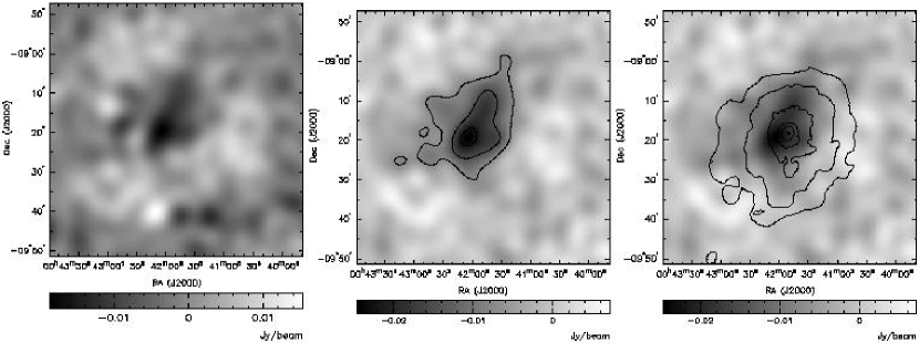
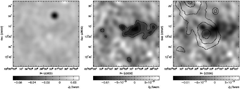
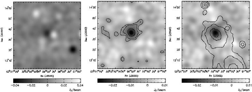
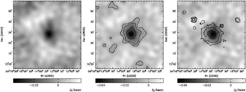
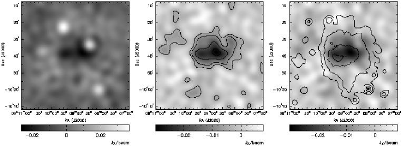
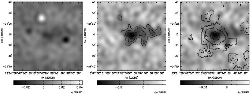
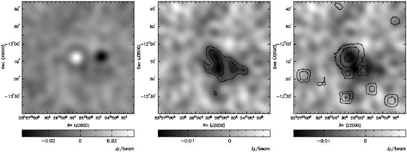
Radio point sources present in all of the observations were subtracted through a combination of fitting on the CBI long baselines ( $>2.5$ m) and observations with the OVRO 40-m telescope. We used the 40-m telescope to measure the fluxes of all NVSS sources within 10^′ of the LMT pointing centers. In each cluster there were between 10 to 21 such sources, of which we detected between 1–5 per cluster whose flux had to be subtracted from the CBI visibility data. Outside a 10^′ radius from the pointing centers, we fit for the fluxes of known NVSS sources using the long CBI baselines. Between 7–16 sources were detected in each cluster at the 2.5- $\sigma$ level. Details of the point source subtraction are presented in Section 4.4. Figures 1 to 7 show A85, A399, A401, A478, A754, A1651, and A2597 before and after point source subtraction. The left hand figures are dirty images, and point sources have not been subtracted. The dirty images are often dominated by a small number of bright sources that can mask the presence of both the cluster and fainter point sources. The middle figures show the clusters after point source subtraction, and the images have been deconvolved. The right hand figures show the grayscale from the deconvolved maps with X-ray contours from ROSAT PSPC data (Mason & Myers, 2000).

2.2 Notes on Individual Clusters

2.2.1 A85

We observed A85 over 11 nights between July and December 2000. X-ray observations show that A85 has a central cooling flow, but this cluster also shows signs of merger activity. There is a smaller group of galaxies just south of the cluster, which can be seen in the X-ray contours. ASCA and BeppoSAX temperature maps show that this “southern blob” is slightly hotter than the rest of the cluster, indicating that it is likely interacting with the cluster, rather than a foreground projection (Markevitch et al., 1998; Lima Neto et al., 2001). If the subcluster were independent, one would expect it to be cooler than the main cluster given its smaller size. Kempner et al. (2002) study the merger of the subcluster in detail through Chandra observations. Lima Neto et al. (2001) determine an overall temperature for the cluster of 6.6 $\pm$ 0.3 keV, in agreement with the ASCA and De Grandi & Molendi (2002) results.

VLA observations show some extended emission from a very steep spectrum radio source (VSSRS) just southwest of the cluster center at 333 MHz (Bagchi et al., 1998; Lima Neto et al., 2001). Although there is a brighter patch in the CBI map at this location, one would not expect to see emission from the VSSRS at 31 GHz. Bagchi et al. (1998) measure a flux of 3.15 $\pm$ 0.15 Jy at 326.5 MHz. If we extrapolate the spectral index of $\alpha=-2.97$ between 300 MHz and 3 GHz, we expect a flux at 31 GHz of 4 $\mu$ Jy, and the bright blob in the CBI map is more likely a CMB hot spot. The presence of the VSSRS, however, indicates a possibility of Compton scattering from relativistic non-thermal electrons in this region. See Section 4.5.4 for details on how this could affect our $H_{0}$ derivation.

We take the ROSAT HRI centroid of 00:41:50.94, $-$ 9:18:10.7 (J2000) (Prestwich et al., 1995) to be the location of SZE centroid in our fits. Of all the clusters presented here, A85 has the largest number of radio point sources (21 at 1.4 GHz to 2.5 mJy) within 10^′ of the cluster center.

2.2.2 A399/A401

We observed A399 and A401 over 6 nights during October and November 2000. A399 and A401 are a pair of clusters which are close together on the sky and in redshift. X-ray observations indicate that the clusters likely have interacted in the past or are currently interacting (Fujita et al., 1996; Fabian et al., 1997). The scenario favored by Fabian et al. (1997) is that the clusters collided some time in the past, disrupting their respective cooling flows, features which are normally associated with clusters containing cD galaxies. The collision could also be responsible for the radio halo associated with A401. The halo has a steep spectrum $\alpha\sim-1.4$ and a total flux density of 21 mJy at 1.4 GHz (Bacchi et al., 2003). Extrapolating the spectral index to 31 GHz, the halo would have a flux of 0.3 mJy at the CBI frequencies and is not expected to be a significant source of contamination. A nonthermal SZE from the halo electrons is possible but difficult to quantify (see Section 4.5.4).

The clusters are separated by only about 30^′, which is smaller than the CBI primary beam. The primary beam attenuates the cluster signal so much that the companions do not appear in the respective maps, but we take into account the presence of the A401 when fitting for $H_{0}$ from the A399 data, and vice versa.

The cluster pair has several very bright radio sources in the field of view and appear very “dirty” in the unsubtracted CBI maps. However, those sources can be accurately fitted out. (See Section 4.4 for details). There is a bright spot SW of A399 that appears in the A399 map at 10.1 mJy which does not correspond to any NVSS sources. It is possible this is an inverted spectrum source which falls below the NVSS detection limit at 1.4 GHz. If that is the case, its spectral index would be $\alpha>0.45$ , which is reasonable considering the distribution of spectral indices we discuss in Section 4.4. If we assume it is a genuine source and we fit for its flux, our $H_{0}$ result changes by $<6$ %, a small amount compared to the uncertainty from the CMB.

2.2.3 A478

We observed A478 over 11 nights during February, November, and December 2000. A478 is one of the most X-ray luminous clusters in the sample. It has very little point source contamination, and its X-ray profile is extremely regular. A478 is the largest cooling flow cluster within $z<0.1$ (White et al., 1994), an indication of its relaxed state. From the ROSAT HRI observations, White et al. (1994) find the centroid of the X-ray emission to be RA=04:13:25.5, Dec=10:27:58 (J2000). Although we have used slightly different coordinates as our pointing center, in our analysis, we take this position to be the centroid of the SZE emission as well. A478 is one of the cleanest clusters in our sample in terms of point source contamination. There are very few central sources, and a very small number of sources at large radius whose fluxes need to be fitted.

2.2.4 A754

We observed A754 over 15 nights during February, October, and November 2000. A754 is an irregular cluster which is considered to be a prototypical merging system (e.g., Henry & Briel, 1995; Henriksen & Markevitch, 1996). Although we have included this cluster in our sample to maintain completeness, we recognize that such a disturbed cluster could contribute biases of its own. In the final sample, we therefore present values of $H_{0}$ with and without A754.

The cluster is also known to have a strong radio halo. At 74 MHz and 330 MHz, the halo flux is 4 Jy and 750 mJy, respectively (Kassim et al., 2001). Bacchi et al. (2003) find a flux of 86 mJy at 1.4 GHz, and a spectral index of $\alpha=1.5$ from comparisons to observations at 330 MHz. Assuming this spectral index, we would expect the halo flux at 31 GHz to be 0.8 mJy.

A754 is very heavily contaminated with bright point sources. One source in particular about 15^′ NW of the cluster appears in the CBI map not to be well subtracted. This is most likely due to the fact that a spherical $\beta$ -model is not a good approximation to this elliptical disturbed cluster, leaving a 10 mJy residual in the point source fit. The level of subtraction for this particular source does not change the value of $H_{0}$ determined for this cluster.

2.2.5 A1651

We observed A1651 over 8 nights during February 2000 and April and May 2001. A1651 appears to be a dynamically relaxed cD cluster with a regular ROSAT PSPC profile (Gonzalez et al., 2000; Markevitch et al., 1998, e.g), However, in their analysis of ASCA observations, Markevitch et al. (1998) find that a cooling component is not required in the fit. This cluster appears to be unremarkable, although it has a large number of bright point sources which need to be subtracted from the CBI data.

2.2.6 A2597

We observed A2597 over 5 nights during September, October, and November 2000. A2597 is another regular cD cluster with a cooling flow. Its X-ray luminosity is among the weakest in our sample, and the SZE maps indicate this. Our detection is marginal at best, and the error in deriving $H_{0}$ from this cluster is large. Sarazin & McNamara (1997) take the centroid of the cluster to be the position of the central cD galaxy (23:25:19.64, $-$ 12:07:27.4, J2000), which we also use as the centroid in the SZE fits. The cD galaxy is a strong emitter at 31 GHz. We determine a flux for the central source of 40 mJy, both from the OVRO 40-m and the CBI long baselines ( $>$ 3 m), giving us confidence in our measurement.

3 Analysis Method

3.1 Modeling the Cluster Gas

We assume that the cluster gas is well fitted by a spherical isothermal $\beta$ -model (Cavaliere & Fusco-Femiano, 1976) . We will discuss possible implications of this assumption later in the paper. The gas distribution is assumed to follow the form

n_{e}(r)=n_{e0}\left(1+\frac{r^{2}}{r_{0}^{2}}\right)^{-3\beta/2},

(1)

where $n_{e0}$ is the central electron density, $r_{0}$ is the physical core radius (related to the angular core radius, $\theta_{0}$ , by $r_{0}=D_{A}\theta_{0},$ where $D_{A}$ is the angular diameter distance to the cluster), and $\beta$ is the power law index. The electron temperature $T_{e}$ is taken to be a constant.

As discussed in Section 1, the X-ray surface brightness from thermal bremsstrahlung radiation is given by

b_{X}(E)=\frac{1}{4\pi(1+z)^{3}}\int n_{e}^{2}(r)\Lambda(E,T_{e})\,dl

(2)

(e.g., Birkinshaw, 1999). Under the assumption of isothermality in the cluster, $\Lambda(E,T_{e})$ is a constant. Assuming spherical symmetry and substituting Eq. 1, this integral becomes

b_{X}\propto n_{e0}^{2}\theta_{0}D_{A}\left(1+\frac{\theta^{2}}{\theta_{0}^{2}}\right)^{-3\beta+1/2}.

(3)

Because surface brightness is independent of distance, and $D_{A}\propto h^{-1}$ , Eq.3 indicates that our measurement of $n_{e0}\propto h^{1/2}$ (since $b_{X}$ and $\theta_{0}$ are constant).

The SZE signal is given by

\Delta I_{\rm SZE}\propto T_{e}\int n_{e}\,dl.

(4)

Again substituting Eq. 1, this integral becomes

\Delta I_{\rm SZE}\propto T_{e}n_{e0}\theta_{0}D_{A}\left(1+\frac{\theta^{2}}{\theta_{0}^{2}}\right)^{-\frac{3}{2}\beta+\frac{1}{2}}.

(5)

Given the above dependences on $h$ of $n_{e0}$ and $D_{A}$ , one can see that the SZE intensity, $\Delta I_{\rm SZE}\propto$ $h^{-1/2}$ . Therefore, if the density profile and electron temperature can be obtained from X-ray observations and the SZE decrement can be measured, one can determine the Hubble constant. $\Delta I_{\rm SZE}$ is our main “observable,” and $h^{-1/2}$ is the quantity we obtain from each individual cluster measurement. For the most part, the main sources of error are symmetric (and approximately Gaussian) in $h^{-1/2}$ , but not in $h$ . Since $h$ has a non-linear relationship to our observable, we cannot average individual values of $h$ for the sample and obtain meaningful errors. Instead, we average together $h^{-1/2}$ from the individual clusters to get a sample value of $h^{-1/2}$ , which we then convert to $h$ for the final measurement.

3.2 Determining cluster parameters from X-ray data

We combine density profile results from ROSAT (Mason & Myers, 2000) with temperature measurements from ASCA (Markevitch et al., 1998; White, 2000) and BeppoSAX (De Grandi & Molendi, 2002). The ROSAT PSPC has a spatial resolution of 30^′′ FWHM and a field of view of 1.5 degrees in diameter, which makes it well-suited for observations of the low-redshift clusters in our sample. At a redshift of 0.05, the field of view corresponds to 3.7 $h^{-1}$ Mpc, which is significantly larger than the expected virial radius for the clusters. Due to its small energy range (0.1–2.4 keV) and spectral resolution, it is not possible to obtain sufficiently accurate temperatures from ROSAT data. XMM-Newton and Chandra are ideal for determining both accurate density and temperature profiles, and we will combine those spectral imaging data with our SZE observations in a future paper. Here, we use published data from ASCA and BeppoSAX observatories, which both have energy ranges from 1–10 keV, making them useful for determining temperatures of the hot gas in galaxy clusters.

3.2.1 Cluster Density Profiles

Mason & Myers (2000, hereafter MM2000) derived density profiles for 14 of the clusters in our sample using archival ROSAT PSPC data. The parameters $\beta$ and $\theta_{0}$ can be derived by fitting a $\beta$ -model surface brightness profile to the X-ray observations:

I(\theta)=I_{0}\left(1+\frac{\theta^{2}}{\theta_{0}^{2}}\right)^{-3\beta+1/2}.

(6)

The $\beta$ -model density normalization, $n_{e0}$ , can be calculated from the total X-ray flux measured over the observed bandpass; see MM2000 for details. Table 3 lists the best fit model parameters from MM2000 which we use in our SZE analysis. MM2000 present 2 different models for clusters which appear to have a cooling flow. In their primary models, the X-ray emission is fit with a $\beta$ -model component plus a gaussian for the cooling flow. In their alternate models, the central region of cluster emission is excised to remove contamination from the cooling flow, which because of its compact size, contributes negligibly to the SZE analysis. We present results using the MM2000 primary models here, but we note that the final results change very little ( $<0.3\sigma$ ) when the alternate models are used. Please see MM2000 for details of the X-ray modelfitting. Note that MM2000 assumed $q_{0}=1/2$ , and in some cases, they used slightly different redshifts and electron temperatures from what we assume in this paper. To account for these differences, we have recalculated the $n_{e0}$ normalization values using the method described in MM2000. We used redshifts from the compilation of Struble & Rood (1999).

3.2.2 Cluster Temperatures

Cluster temperatures $T_{e}$ can be determined through spectral modeling, where high-resolution X-ray spectra are fitted with a thermal emission model for a low-density plasma in collisional ionization equilibrium (i.e., the $mekal$ or Raymond-Smith models in XSPEC), which has been absorbed by Galactic hydrogen. If an X-ray detector has sufficient spatial resolution, such as XMM-Newton or Chandra , temperature profiles can be measured by binning the spectral data into different regions across the detector. Here, we rely on published ASCA and BeppoSAX results. ASCA has an energy dependent PSF which makes it difficult to obtain accurate temperature profiles from the data. Single emission weighted temperatures over the entire cluster derived from ASCA should be reliable, and we use these as estimates for “isothermal” temperatures in our SZE analysis. BeppoSAX has good spatial resolution (1^′) and a better understood PSF, making it a better candidate for determining temperature profiles. BeppoSAX results are available for 2 clusters whose results are reported here. De Grandi & Molendi (2002) report average temperatures for the clusters, excluding cooling flow regions. Where available, we combine these with the ASCA results, and in Section 4.3 we use their mean profile results to determine the magnitude of error we might expect from our isothermal assumption.

Table 4 lists temperature results obtained from ASCA data by Markevitch et al. (1998) and White (2000). The results are in fair agreement, except for the cooling flow clusters, where assumptions used in the energy-dependent PSF matter more. Until we can conclusively resolve these discrepancies using observations from current missions, we adopt the average of the results from both these papers. Given that the results are based on the same observational data, the errors are likely to be correlated. As a conservative estimate of the error in the mean of the temperatures, we use the larger of the two sets of error bars, and we include an extra component to the uncertainty to account for systematic offsets between the two measurements. Note that Markevitch et al. (1998) quote 90% confidence errors, while White (2000) uses 68% confidence intervals. For consistency, we convert Markevitch et al. (1998) errors to 68% confidence. Since we do not have knowledge of the actual likelihood distribution, we assume a Gaussian distribution, symmetrize the errors, and scale them by 1.65. Two of the clusters here have BeppoSAX observations which have been analyzed in detail (De Grandi & Molendi, 2002). These results are independent of the ASCA temperatures, and Table 4 shows them to be in excellent agreement. Where available, we average the BeppoSAX temperatures with the mean ASCA temperatures. The temperatures and errors we assume are listed in Table 4.

3.3 Modeling the expected SZE profile

Including relativistic effects, the thermal SZE for an isothermal cluster can be represented by

\frac{\Delta I_{\rm SZE}}{I}=\tau\frac{xe^{x}}{e^{x}-1}\left\{\frac{k_{b}T_{e}}{m_{e}c^{2}}(F-4)+\left(\frac{k_{b}T_{e}}{m_{e}c^{2}}\right)^{2}\left[-10+\frac{47}{2}F-\frac{42}{5}F^{2}+\frac{7}{10}F^{3}+\frac{7}{5}G^{2}(-3+F)\right]\right\}

(7)

(Sazonov & Sunyaev, 1998; Challinor & Lasenby, 1998). $I$ is the CMB intensity, $\Delta I_{\rm SZE}$ is the change due to the SZE, $k_{b}$ is the Boltzmann constant, $m_{e}$ is the electron mass, and $c$ is the speed of light; $\tau$ is the optical thickness to Compton scattering given by $\tau=\int\sigma_{T}n_{e}(l)dl$ , and $\sigma_{T}$ is the Thomson scattering cross section; $x$ represents the frequency of observation, scaled as $x=\frac{h\nu}{k_{b}T_{CMB}}$ , with $\nu$ being the observing frequency and $T_{CMB}=2.725\pm 0.001$ K (Fixsen & Mather, 2002); $F=x\coth(x/2)$ and $G=x/\sinh(x/2)$ . The first term in Eq. 7 ( $\propto\frac{k_{b}T_{e}}{m_{e}c^{2}}$ ) represents the original thermal SZE described by Sunyaev & Zel’dovich (1972). Rephaeli (1995) showed that the relativistic velocities of electrons in the hot gas of galaxy clusters must be taken into account when measuring the SZE. The second term in Eq. 7 ( $\propto\left(\frac{k_{b}T_{e}}{m_{e}c^{2}}\right)^{2}$ ) is the relativistic correction (Sazonov & Sunyaev, 1998; Challinor & Lasenby, 1998). This analytical expression for the correction has been shown to be in good agreement with numerical results of Rephaeli (1995). For cluster gas with temperatures in the range of our sample ( $T_{e}\sim 4-10$ keV), the relativistic term amounts to $\sim$ 3% downward correction in the magnitude of the predicted SZE at our frequency of observation.

We can factor out one $\left(\frac{k_{b}T_{e}}{m_{e}c^{2}}\right)$ and rewrite Eq. 7 as:

\frac{\Delta I_{\rm SZE}}{I}=\frac{k_{b}T_{e}}{m_{e}c^{2}}\sigma_{T}f(x,T_{e})\int n_{e}\,dl

(8)

where $f(x,T_{e})$ is $\frac{xe^{x}}{e^{x}-1}$ multiplied the expression in brackets (divided by $\frac{k_{b}T_{e}}{m_{e}c^{2}}$ ) from Eq. 7. From Eq.1 we obtain the expected SZE profile,

\frac{\Delta I_{\rm SZE}}{I}(\theta)=\frac{k_{b}T_{e}}{m_{e}c^{2}}\sigma_{T}f(x,T_{e})n_{e0}\sqrt{\pi}\frac{\Gamma(\frac{3\beta}{2}-\frac{1}{2})}{\Gamma(\frac{3\beta}{2})}D_{A}\theta_{0}\left(1+\frac{\theta^{2}}{\theta_{0}^{2}}\right)^{-\frac{3}{2}\beta+\frac{1}{2}}.

(9)

As we discuss later, the CMB contamination is sufficiently large that we cannot accurately determine the $\beta$ -model parameters from the CBI data. The parameters are, however, very well constrained by the ROSAT imaging observations, and we hold the model parameters fixed. For each CBI frequency channel, Eq. 9 can then be reduced to

\Delta I_{\rm SZE}(\theta)=I_{0}\left(1+\frac{\theta^{2}}{\theta_{0}^{2}}\right)^{-\frac{3}{2}\beta+\frac{1}{2}},

(10)

where $I_{0}(\propto h^{-1/2})$ is a constant.

An interferometer measures the Fourier transform of this profile multiplied by the primary beam of the telescope:

V(u,v)=I_{0}\int_{-\infty}^{\infty}\int_{-\infty}^{\infty}B(\theta)\left(1+\frac{\theta^{2}}{\theta_{0}^{2}}\right)^{-\frac{3}{2}\beta+\frac{1}{2}}e^{2\pi i(ux+vy)}\,dx\,dy,

(11)

where $x$ and $y$ are positions on the sky ( $\theta^{2}=x^{2}+y^{2}$ ), and $u$ and $v$ are the visibility positions in units of wavelength. Details of the CBI primary beam, $B$ , are presented in Pearson et al. (2003). We fit the visibility model in Eq. 11 to the observed CBI data by minimizing $\chi^{2}$ with respect to $I_{0}$ to obtain the best-fit SZE decrement and $h^{-1/2}$ . The best-fit visibility profiles are plotted with the radially averaged, point source subtracted CBI data in Figure 8. Table 7 lists results from the fits to the CBI observations in mJy arcm^-2 and gives the $\chi^{2}$ values for the fits.

In the context of interferometer observations, it is convenient to use intensity units of Jy sr^-1, but more traditional single dish observations quote SZE decrements in $\mu$ K. We use

\Delta I_{\rm SZE}=\frac{2\nu^{2}kT_{CMB}}{c^{2}}\frac{x^{2}e^{x}}{(e^{x}-1)^{2}}\frac{\Delta T}{T_{CMB}}

(12)

to convert from intensity to $\mu$ K. Table 9 lists results from the fits to the CBI observations in $\mu$ K, and gives the $\chi^{2}$ values for the fits. Another useful quantity is the Compton- $y$ parameter, defined as

y=\frac{k_{b}T_{e}}{m_{e}c^{2}}\tau,

(13)

which is independent of the frequency of observation. We list $y_{0}$ , the central Compton- $y$ value for each cluster in Table 9.

4 Error Analysis

The analysis method described above makes several idealizing assumptions about galaxy clusters - that they are spherical, smooth, and isothermal. In this section we discuss possible implications of deviations from these assumptions. So far, we also have not considered effects of contaminating factors such as observational noise, CMB primary anisotropies, foreground point sources, non-thermal radio emission from relics or haloes, and kinematic SZE signals from peculiar velocities. We address all these different sources of error in this section. Since the SZE model-fitting is performed in the visibility domain (the Fourier transform of the image plane), the error sources have relationships which are not analytical and whose interpretations are not always intuitive. Therefore, to characterize their effects, we use Monte Carlo simulations, mimicking the real observations and various error sources.

In the simulations, we attempted to reproduce as accurately as possible all the components that enter a real CBI observation. We derived an SZE model “image” using the cluster gas parameters obtained from the X-ray data as described in Section 3.3. We multiplied the image by the CBI primary beam, and performed a Fourier transform to obtain our simulated model visibility profile. We used the observed CBI visibility data as a template, maintaining identical $u-v$ coverage to the real observation by replacing the observed visibility data with the simulated data and randomizing the visibilities with the observed level of Gaussian thermal noise. We then analyzed each mock data set in the same way as the actual observation, fitting for the “observed” SZE decrement. We repeated this process $10^{3}$ times for each cluster, randomizing the thermal noise and the error source whose impact we were attempting to quantify. This yielded a distribution of best-fit $I_{0}$ ’s, which is equivalent to the distribution of $h^{-1/2}$ for that error source, which we use to obtain 68% confidence intervals. As we discuss below, several sources of error are not independent, and must be considered together in the Monte Carlo simulations. The largest source of random error is the intrinsic CMB anisotropy. It has a significant impact on almost all the other error sources, so we include it in most of the other simulations.

4.1 Intrinsic CMB Anisotropies

The CBI has measured the CMB on arcminute scales, finding bandpower levels of 2067 $\pm$ 375 $\mu$ K² at $\ell\sim 600$ (1 m baseline), and 1256 $\pm$ 284 $\mu$ K² at $\ell\sim 1200$ (2 m baseline) (Pearson et al., 2003). Figure 8 shows that the SZE cluster signal is strongest on the 1 m and 2 m baselines, where the CMB is a significant contaminant. The SZE data is effectively radially averaged in the visibility fitting, and the rms of the CMB averaged in this way on the 1 m and 2 m baselines is 30 mJy and 7 mJy, respectively. We cannot remove the intrinsic CMB anisotropies from our data without observations at other frequencies, so we need to measure its impact on our results. We generated $10^{3}$ randomized realizations of the CMB primary anisotropies, using the algorithm described in Appendix A. Each of these “sky” realizations was then added to the simulated clusters described above, and we fitted for the value of $h^{-1/2}$ which minimized $\chi^{2}$ . The input power spectrum we used is the best fit model to the CBI power spectrum observations, combined with Boomerang-98, DASI, Maxima, VSA, and COBE DMR measurements (Sievers et al., 2003): $\Omega_{\rm tot}=1.0$ , $\Omega_{b}h^{2}=0.02$ , $\Omega_{\rm cdm}h^{2}=0.14$ , $\Omega_{\Lambda}=0.5$ , $n_{s}=0.925$ , $\tau_{c}=0$ , ${\cal C}_{10}=887$ $\mu$ K². We list in Table 8 the 68% confidence intervals in $h^{-1/2}$ for each cluster, given the expected levels of CMB contamination based on the CBI’s power spectrum measurements. The average fractional error in $h^{-1/2}$ per cluster due to the CMB is 36%, and this clearly dominates all other sources of uncertainty.

4.2 Density model errors

Because the CMB contamination is so large, it is not meaningful to fit for the shape of the cluster gas profile from the SZE data. We therefore assume that the profile we derived from the X-ray data is correct, and hold the $\beta$ -model parameters fixed. Here, we quantify errors due to possible deviations from this best fit X-ray model. To determine the error in the individual cluster density profile parameters MM2000 also used Monte Carlo simulations. For each cluster, they smoothed the original composite 0.5-2.0 keV count-rate image using a 30^′′ FWHM Gaussian. A set of $10^{3}$ simulated observations were then created by multiplying the smoothed image by the exposure maps and adding random Poisson noise. For each simulated observation, they applied the same analysis procedure that was used to determine the cluster parameters from the original data set. We use their resulting distribution of $\beta$ -model parameters, $\beta$ , $\theta_{0}$ , and $n_{e0}$ to determine the expected error in $h^{-1/2}$ due to possible ambiguities in the density profile modeling for each cluster. We generated $10^{3}$ simulated CBI data sets using the different $\beta$ -model parameter trios from the simulated X-ray observations to generate slightly different SZE profiles. We then fitted for the SZE decrement $\Delta I$ using the best fit X-ray parameters from the original ROSAT image. The resulting distribution in $h^{-1/2}$ provides expected errors due to possible inaccuracies in the density profile modeling. Because the X-ray emission and SZE have different dependences on the model parameters, there is a slight bias in the SZE distribution relative to the X-ray distributions. We discuss this bias in Appendix B and list the results in Table 8. The bias corrections are mostly negligible ( $<$ 1%), but A754, a highly disturbed cluster with a larger degree of model parameter uncertainty, requires a correction of 3.6%.

4.3 Temperature Profiles

Our analysis also assumes that cluster gas is isothermal. If this assumption is correct, determining errors from inaccuracies in the value of $T_{e}$ is straightforward; $h^{-1/2}$ is simply proportional to $T_{e}$ . Whether the gas is in fact isothermal has been the subject of ongoing debate. In their analysis of the same ASCA data, Markevitch et al. (1998) find temperature profiles which decline with radius, while White (2000) finds isothermal profiles. De Grandi & Molendi (2002) also find declining profiles from their analysis of BeppoSAX data, but they find that the profiles have a slightly different slope and break radius from the Markevitch et al. (1998) profiles. XMM-Newton observations indicate that individual clusters may vary; A1795 has a temperature profile consistent with isothermal out to 0.4 $r_{\rm vir}$ while Coma shows a declining temperature profile (Arnaud et al., 2001c, a). Departures from isothermality can produce large errors in the derivation of $H_{0}$ from the X-ray/SZE method if an isothermal model is assumed, but the magnitude of the error depends on many factors.

To estimate the possible effect of an inaccurate temperature profile, we study the case of gas modelled as a hybrid isothermal-polytropic temperature profile, where the temperature is uniform out to a radius $r_{\rm iso}$ , and declines outside this radius. This model was introduced by Hughes et al. (1988) and is similar to the profile found by Navarro et al. (1995) in N-body simulations. It is represented by

T(r)=\left\{\begin{array}[]{ll}T_{0}&\mbox{if }r\leq r_{\rm iso}\\ T_{0}\left(\frac{n(r)}{n(r_{\rm iso})}\right)^{\gamma-1}&\mbox{if }r>r_{\rm iso}\end{array}\right..

(14)

Theoretical calculations disagree on where the transition radius $r_{\rm iso}$ should occur, although it is generally taken to be of order a virial radius, $r_{\rm vir}$ , which we approximate as $r_{200}$ , defined in the manner of Evrard et al. (1996) as the radius which encloses a mean density 200 times the cosmological critical density.

In the limit where $r_{\rm iso}=0$ , the temperature profile is simply a polytropic model. We expect $1<\gamma<5/3$ , where $\gamma=1$ is the isothermal limit, and $\gamma=5/3$ is the adiabatic limit. The expected central SZE decrement depends fairly strongly on $\gamma$ and $r_{\rm iso}$ , but the effect of these parameters on the derivation of $H_{0}$ using interferometric SZE data is not completely straightforward. A hybrid temperature profile will cause two changes relative to an isothermal model. The overall decrement will be smaller, and the cluster will appear more compact. The interferometer measures visibilities which are the Fourier transform of the image, so a steep image profile will have a shallower visibility profile and vice versa. Because the visibility profile shallows as $r_{\rm iso}$ is decreased, the hybrid profiles cross the isothermal profile at different points. Therefore, it is difficult to know whether we will overpredict or underpredict $H_{0}$ for different clusters without an accurate temperature profile.

We demonstrate this with a simulation which is summarized in Table 5. We generated false SZE data sets using hybrid models with different pairs of $\gamma$ and $r_{\rm iso}$ where the input models all assumed $h=1$ . For each model, we rescaled $T_{0}$ such that the emission weighted temperature for that model agreed with the observed value. We then fitted an isothermal profile to the hybrid model data to determine the error in deriving $H_{0}$ due to the temperature profile. Table 5 lists our results for A478. We see that for steeply declining profiles, our error in $h$ will be very large, and can be incorrect by a factor of 2 in the most extreme case. Some cases supported by observational data include $r_{\rm iso}=0$ , $\gamma=1.2$ (Markevitch et al., 1998) and $r_{\rm iso}=0.2$ , $\gamma=1.5$ or $\gamma=1.2$ for non-cooling flow and cooling flow clusters respectively (De Grandi & Molendi, 2002), where $r_{\rm iso}$ is in units of $r_{200}$ . If the Markevitch et al. (1998) profile is correct, then we overestimate $h$ from A478 by 22%; if the De Grandi & Molendi (2002) profile is correct, then our value of $h$ is largely unaffected by the temperature profile. The errors can be very different for different clusters, and in some cases go in the opposite direction, where $h$ is underestimated for steeply declining temperature profiles. We summarize in Table 6 the levels of error expected if the mean ASCA and BeppoSAX profiles apply to each of our clusters. For the De Grandi & Molendi (2002) profiles, we have boldfaced the relevant column, based on whether a particular cluster is believed to have a cooling flow or not. Depending on which mean profile is assumed, for the sample of 7 clusters presented here, our value of $h$ may be essentially correct, with an overestimate of only 1% based on the Markevitch et al. (1998) profile, or it could be underestimated by 14% assuming the De Grandi & Molendi (2002) mean profiles. This demonstrates that an accurate knowledge of the temperature profile is important for eliminating a bias in $H_{0}$ from non-isothermal cluster temperatures. To determine $r_{\rm iso}$ and $\gamma$ , the profiles need to be probed to a large radius, typically tens of arcminutes for our clusters, which means that Chandra observations alone are usually not adequate for these purposes.

4.4 Errors from Foreground Point Sources

Foreground point sources are the largest source of contamination in CMB experiments at 30 GHz. We hope to limit the point source error in our $H_{0}$ determination to $<2\%$ for the sample of 15 clusters, or $<8\%$ per cluster. Our strategy for removing point source contamination involves a combination of fitting for the fluxes of sources at known positions simultaneously with the cluster model, and independently measuring some source fluxes with the OVRO 40-m telescope and the VLA. The CBI short ( $\leq$ 2 m) baselines are most sensitive to the signal from the extended cluster and CMB primary anisotropies. The strength of the cluster and CMB both decline significantly on longer baselines, making those baselines suitable for determining point source fluxes. However, this source fitting is not reliable for sources near the cluster center, and we use independent observations to accurately determine their fluxes. The advantage of fitting the source fluxes using the CBI data is that the point source and cluster observations are simultaneous, so source variability is not an issue, although most point sources in clusters are steep spectrum and non-varying (e.g. Slingo, 1974; Cooray et al., 1998). The disadvantage is that for sources close to the cluster center (also the pointing center of the observation), the point source appears as an overall offset on all baselines in the visibility domain where we perform the fitting. The overall offset from the point source is difficult to distinguish from the cluster signal, especially in the less resolved, compact clusters such as A478 and A401, resulting in large errors in the $H_{0}$ analysis. We find that sources close to the cluster center within about 10^′ need to be observed independently with very high accuracy (about 1 mJy rms at 31 GHz), and sources outside this radius can be safely fitted using the CBI long baselines. We fit sources outside the 10^′ radius that have fluxes detectable at the 2.5- $\sigma$ limit, and we account for the contribution of the remaining (unfitted and unsubtracted) sources statistically using Monte Carlo simulations which we describe below. As a basis for our study, we use the NVSS catalog, which is complete to 2.5 mJy at 1.4 GHz. We assume that all relevant sources at 30 GHz are in the NVSS catalog and that we do not miss any sources with inverted spectral indices. This assumption is supported by our OVRO study and VLA X-band survey of one of the blank CMB fields, as well as a study of point sources in the CBI Deep fields (Mason et al., 2003). Although Taylor et al. (2001) do find from their 15 GHz survey a large chance of missing inverted spectrum sources from extrapolations from low frequency, we estimate based on their source counts that the probability of such a source occuring in the crucial central 10^′ of our cluster centers is low. Sources outside this radius do not contribute a significant error, as we explain below.

To test our source subtraction method and quantify errors, we generated simulated cluster observations using the X-ray derived density models described above, including realistic thermal noise and CMB primary anisotropies. We added all NVSS sources (down to 2.5 mJy at 1.4 GHz) to each simulated cluster realization at the listed NVSS positions, but we varied the fluxes for each iteration by randomly selecting spectral indices from the distribution observed by Mason et al. (2003) to determine the source fluxes at each of the CBI channels from 26 to 36 GHz. We then defined specific criteria to determine how the different sources would be treated in the analysis.

If a source was within 10^′ of the LMT pointing centers, we “subtracted” the source, assuming its flux is known to a certain rms from an independent telescope. In the simulations we added at these source positions, random Gaussian noise with an rms equivalent to the levels observed with the OVRO 40-m telescope. The sensitivity achieved with the 40-m varied from 0.4 to 2.0 mJy rms for individual sources. The simulations show that these central point sources observed with the 40-m contribute $\sim$ 10% error per cluster.

If a source was outside the 10^′ radius and could be detected at the 2.5- $\sigma$ level on baselines longer than 2.5 m, we fitted for the flux of the source simultaneously with the cluster. Before selecting the 2.5- $\sigma$ sources in the simulations, we added random fluctuations to the source fluxes to simulate possibly missing some sources due to noise. All other sources were ignored (i.e., not subtracted or fit for in any way). In the fitting, we fixed the source positions to the NVSS coordinates, which is reasonable since the rms error in the NVSS positions ranges from $<1-7^{\prime\prime}$ , much smaller than the CBI synthesized beam of a few arcminutes. We found that it was extremely inefficient to fit for the spectral indices of large groups of point sources over the CBI 10 GHz bandwidth, so we fixed them at the weighted mean value of the distribution found by Mason et al. (2003), $\alpha=-0.55$ . To determine whether this assumption affects our results, we also tried fixing the spectral index to $\alpha=0$ . We found that the $H_{0}$ results change by $<1$ % in all cases. In the simulations the small number of sources whose fluxes are determined from the CBI data itself (typically 10-15 per cluster) contribute a negligible amount of error to the $h^{-1/2}$ fits.

All sources that were outside the 10^′ radius and were not at least 2.5- $\sigma$ were ignored in the SZE fitting. We compare these simulations with those described in Section 4.1, where only observational noise and CMB anisotropies are added. The $10^{3}$ Monte Carlo iterations show that the unsubtracted sources contribute a small but consistent bias, tending to make the mean $h^{-1/2}$ for a cluster higher or lower, depending on the configuration of residual sources present in the LMT fields. The bias from the unsubtracted sources is an additive factor, and the values for the individual clusters are listed in Table 8. All are $<$ 3%.

The spectral index distribution determined by Mason et al. (2003) was derived for observations of cluster-free CMB fields. The point source populations in galaxy clusters can be considerably different, and have not been well studied at 30 GHz. Cooray et al. (1998) find a distribution of $-0.77\pm 0.48$ , which is somewhat different from the Mason et al. (2003) distribution. We retest our method using the Cooray et al. (1998) distribution instead of the Mason et al. (2003) distribution, and find the results to be almost unchanged. The sample value of $h^{-1/2}$ changes by $<$ 0.3%, and the magnitude of the sample error changes by $<$ 1%.

4.5 Other error sources

4.5.1 Asphericity

Because of the CMB contamination, we cannot meaningfully study the cluster shapes as seen in the SZE from the CBI data. Any errors in $h^{-1/2}$ from slight pointing inaccuracies on the level seen in the CBI, offsets in $x,y$ from the assumed cluster center up to a few arcminutes, or ellipticity in the plane of the sky are all dwarfed by the CMB, so we ignore them here. The 2-D shapes of clusters seen in X-ray emission provide a good indicator of the level of expected asphericity. Cooray (2000) has analyzed the 2-D distribution of X-ray cluster shapes observed by Mohr et al. (1995), showing that for a sample of 25 clusters randomly drawn from an intrinsically prolate distribution, the error in $H_{0}$ for the sample is less than 3%. Therefore, for our complete sample, we do not expect a large systematic error due to cluster asphericity. We estimate the uncertainty in $H_{0}$ for each cluster by taking 3% $\times\sqrt{25}$ = 15%, so the uncertainty for each cluster in $h^{-1/2}$ $\sim 7.5$ %. For our primary sample of 15 clusters, the error in $H_{0}$ due to asphericity should be $<$ 4%.

4.5.2 Clumpy gas distribution

In the fitting, we assume that the density distribution is smooth, directly applying the density profile model derived from the X-ray observations to the SZE models. Because the CMB is such a large contaminant, and we cannot meaningfully obtain shape parameters from the SZE data, potential systematic errors due to clumpy gas cannot be addressed with our data and can probably only be understood in detail through hydrodynamical simulations. However, Eq. 2 and Eq. 5 show that $h\propto\langle n_{e}^{2}\rangle/\langle n_{e}\rangle^{2}$ , a quantity which is always greater than unity. Therefore, any clumpiness in the gas distribution will cause one to overestimate $h$ by this factor, although as we saw from our study of different temperature profiles that the analysis for interferometer data could be more complicated than this.

4.5.3 Peculiar Velocities

The expression given for the thermal SZE in Eq. 7 assumes that the cluster is not moving with respect to the Hubble flow. In reality, all clusters have some peculiar velocity $V_{\rm pec}$ , taken to be at an angle $\theta$ relative to the vector drawn from the cluster to the observer. This produces a kinematic SZE given by

\frac{\Delta I_{\rm kin}}{I}=\tau\frac{xe^{x}}{e^{x}-1}\left\{\frac{V_{\rm pec}}{c}\mu+\left(\frac{V_{\rm pec}}{c}\right)^{2}\left(-1-\mu^{2}+\frac{3+11\mu^{2}}{20}F\right)+\frac{V_{\rm pec}}{c}\frac{k_{b}T_{e}}{m_{e}c^{2}}\mu\left[10-\frac{47}{5}F+\frac{7}{10}(2F^{2}+G^{2})\right]\right\}

(15)

(Sazonov & Sunyaev, 1998), where all quantities are as defined in Section 3.3, and $\mu=\cos\theta$ . The first term is the kinematic SZE, which can be positive or negative, depending on whether the cluster is moving away from us or towards us. The second term is a relativistic correction to the kinematic SZE, and the third part of the expression is a cross-term between the thermal and kinematic effects. The last term is the dominant correction to kinematic SZE measurements in single clusters. For our purposes, we can assume that the clusters have random peculiar velocities along our line of sight, and the terms in $V_{\rm pec}/c$ will average out over the sample, although we will consider their contribution to our error budget for each individual cluster below. The $(V_{\rm pec}/c)^{2}$ term will not average out for the sample, but its magnitude is very small, even for large peculiar velocities.

Giovanelli et al. (1998) measured the peculiar velocities of 24 galaxy clusters with radial velocities between 1000 and 9200 km s^-1 ( $z<0.03$ ). None of the peculiar velocities in the CMB reference frame exceed 600 km s^-1, and their distribution has a line of sight dispersion of 300 km s^-1. The mean magnitude of their observed radial peculiar velocities is $\sim$ 200 km s^-1. Slightly larger peculiar velocities are found in numerical simulations created by the Virgo Consortium (e.g., Kauffmann et al., 1999). Colberg et al. (2000) find from the simulations that for haloes with masses comparable to the clusters in our sample ( $M>3.5\times 10^{14}h^{-1}$ M_⊙), the peculiar velocities range from about 100 $-$ 1000 km s^-1 for a $\Lambda$ CDM cosmology, with 11 out of 69 clusters having $V_{\rm pec}>600$ km s^-1. The average peculiar velocity for the $\Lambda$ CDM model is about 400 km s^-1. We calculate the error in $h^{-1/2}$ due to the kinematic SZE for each cluster assuming $V_{\rm pec}=$ 400 km s^-1 and list the values in Table 8. The uncertainties due to peculiar velocities range from 4%–8%. For the weakest cluster in our sample, A2597, a large peculiar velocity of 1000 km s^-1 produces an error in $h^{-1/2}$ of $\sim$ 0.04% from the $(V_{\rm pec}/c)^{2}$ term. Thus, there is no systematic error in the sample from ignoring the kinematic SZE relativistic correction. Errors due to the kinematic/thermal SZE cross term are negligible ( $<0.1$ %) for all cases.

4.5.4 Comptonization due to a nonthermal populations of electrons

Clusters which have recently merged are usually associated with radio relics or haloes. This non-thermal emission can affect our results in two possible ways. If the halo is extremely bright, it can cause contaminating foreground emission at 31 GHz. As noted in the sections on the individual clusters, two clusters discussed in this paper, A401 and A754, have haloes at lower frequencies, but due to their steep spectral indices, we do not expect them to contribute significant flux at 31 GHz. The second possible effect is a contribution to the SZE from the non-thermal population of electrons present in the cluster. Quantifying this effect is very difficult, even with detailed radio, EUV, and X-ray data because the electron population models are not well-constrained by the observational data. Shimon & Rephaeli (2002) have studied four different electron population models that can reproduce observed data from the Coma cluster and A2199. Three of the four models produce a negligible contribution to the total SZE from the non-thermal population of electrons ( $<1$ % in most cases). The fourth model non-thermal electron population contributes 6.8% and 34.5% of the total SZE flux in the two clusters, but that model is deemed to be unviable by the authors because the ratio of the total energy in the non-thermal electrons to that in the thermal electrons is too high to be realistic. One of the three viable models produces a contribution of 3% to the total SZE in A2199. Colafrancesco et al. (2003) also calculate the contribution to the SZE from non-thermal electrons, using fewer approximations than Shimon & Rephaeli (2002). Their results are similar in that the magnitude of the non-thermal SZE is highly dependent on the model used to represent the electron population. Here, we simply note that Comptonization by a non-thermal electron population is a possible source of additional error in our result, although current plausible models indicate that the magnitude of the error may be negligible.

5 Combined Results

To determine the total error for each individual cluster, we can combine independent sources of error by adding them in quadrature if they are Gaussian, or convolving the different likelihood distributions if they are not. However, since all the Monte Carlo simulations depend so heavily on the CMB noise, it is difficult to separate the independent components. For example, the CMB has a large effect on how well the point sources can be fitted, as do the X-ray models. In the point source fitting, we assume we completely understand the shape of the SZE profile based on the X-ray data. If the profile is slightly wrong, this can affect the point source subtraction. We therefore perform a final simulation set where all the major sources of error - CMB, point sources, and X-ray models - are varied simultaneously. Here we only consider the isothermal $\beta$ -models described in MM2000. We list in Table 8 the 68% confidence intervals in $h^{-1/2}$ for each cluster, given the various sources of error. Note that these errors are absolute, not fractional. The reason is that the CMB dominates the error, and it effectively adds or subtracts flux to the cluster and is not a scaling factor, although the fractional expected error in $h^{-1/2}$ is a function of the cluster signal and shape, where brighter, more compact clusters experience less contamination.

The final $h^{-1/2}$ results, corrected for the X-ray model and unsubtracted point source biases, are presented in Table 9 with their 68% random uncertainties from CMB anisotropies, thermal noise, calibration errors, point source subtraction, asphericity, temperature determination (within context of an isothermal model), and peculiar velocities. The final statistical uncertainties were calculated by adding in quadrature the values from the last three columns of Table 8, the 7.5% uncertainty per cluster from asphericity, and the 2% uncertainty per cluster from the radio calibration. Central values of $\Delta T_{0}$ and $y_{0}$ which have also been corrected for the X-ray model and unsubtracted point source biases are listed as well.

As we have emphasized, a major potential bias in determining $H_{0}$ from combined SZE/X-ray observations is asphericity in the clusters. Weighting by the errors could possibly bias the sample average if the magnitudes of the errors correlate with properties of the cluster that relate to the asphericity bias. For example, an elongated cluster oriented along the line of sight would appear more compact than the same cluster oriented perpendicular to the line of sight. Thus, if the magnitudes of the errors in our determination of $H_{0}$ correlate with the sizes on the sky of the clusters, a sample result which has been weighted by the errors could potentially be biased. We determine the apparent sizes of each cluster by calculating the FWHM of the $\beta$ -model. The most compact cluster, A2597, is also one of the least luminous objects in the sample. Since its signal is relatively weak, the error due to CMB contamination is significant. If we exclude this cluster, there is very little correlation between the errors and cluster size, with a correlation coefficient $r=-0.16$ ; with this one anomalous object, $r=-0.58$ .

First, to avoid any possible bias, we simply take a straightforward average of the $h^{-1/2}$ results and errors. The unweighted average is $H_{0}=67^{+30}_{-18}\mbox{}^{+15}_{-6}$ km s^-1 Mpc^-1 for this sample of 7 clusters, where the first set of uncertainties represents the random error at 68% confidence, and the second set represents systematic errors corresponding to calibration uncertainties and possible bias due to a nonisothermal profile, for which we use the average sample biases ( ${}^{+1\%}_{-8\%}$ in $h^{-1/2}$ ) from Table 6. Since we expect the 5% absolute calibration uncertainty to be independent of the nonisothermality bias, we added the two uncertainties in quadrature. As discussed in Section 2.1, A754 is a merging, disturbed cluster. If we exclude it from the final result, we obtain $H_{0}=65^{+34}_{-19}\mbox{}^{+14}_{-6}$ km s^-1 Mpc^-1 from the remaining 6 clusters. Given that the correlation between error and cluster size is not large, we also present a weighted sample average, with the caveat that there is a possibility of the result being biased. The sample average weighted by the errors gives $H_{0}=75^{+23}_{-16}\mbox{}^{+16}_{-7}$ km s^-1 Mpc^-1 .

We use the sample average value to compare the relative magnitudes of the sources of statistical error discussed in Section 4. In Table 8, random errors from the CMB and unsubtracted or incorrectly subtracted point sources are given as absolute errors. This is because the CMB and point sources have a given strength and will cause the same magnitude of error whether the cluster is weak or strong. Random errors from asphericity, electron temperature measurements, peculiar velocity, and radio calibration are all fractional errors. In Table 10, we summarize all the sources of statistical uncertainty, using our sample value of $h^{-1/2}$ $=1.22$ to convert between absolute and fractional uncertainties. We give the average error expected per cluster, as well as the sample average.

There is a large scatter in the individual $h^{-1/2}$ results, but the scatter is entirely consistent with the uncertainties. The mean and standard deviation in $h^{-1/2}$ =1.22 $\pm$ 0.52. For the 7 clusters, the error in the mean is 0.20, which is equal to the sample uncertainty derived from the individual cluster errors of 0.20 from the unweighted average. The reduced $\chi^{2}$ for the sample mean is 1.47 with 6 degrees of freedom, with a probability of 21% of exceeding this value by chance.

The uncertainties in the $H_{0}$ results presented here are dominated by confusion due to the CMB primary anisotropies. In this analysis, when fitting the SZE models to the visibility data, we weight only by the thermal noise. An obvious improvement would be to take advantage of the fact that we know the CMB’s angular power spectrum (Mason et al., 2003; Pearson et al., 2003), and weight the visibility data by the level of power in the CMB on a particular angular scale when performing the modelfitting. However, the errors due to the CMB are highly correlated for visibilities which are close to each other, and this correlation must be removed by diagonalizing the CMB covariance matrix. Details of this method will be described in a future paper . We note here that by using this improved weighting method, the errors in our result above would be reduced by $\sim 30$ % for this sample of 7 clusters.

6 Comparison with Past SZE Observations

Mason et al. (2001) (hereafter MMR) and Myers et al. (1997) observed four of the clusters presented in this paper, A399, A401, A478, and A1651, with the OVRO 5-m telescope. We compare the CBI results with the OVRO 5-m observations. MMR reanalyzed A478 observations taken by Myers et al. (1997), and we use the MMR results here. There are a few differences between the CBI and OVRO 5-m observations which must be taken into account. First, for all 4 clusters, different Lead and Trail fields were observed by the 2 groups. These differing fields contribute significant errors to the results. Also, slightly different redshifts, electron temperatures, and cosmologies were assumed in the 2 analyses. If we take these into account and fit models to the CBI data using all the same parameters assumed by MMR, the results we would obtain are presented in Table 11. Errors from the CMB in the Main fields will be correlated for the 2 observations, since the same patch of CMB is being observed. However, the CMB contribution should not be identical because the interferometer and single dish measurements are sensitive to different modes of the CMB. Calculating the correlated error in the Main field is complicated, so instead we performed the following estimate. We compared our results to those of MMR assuming two different uncertainties. In our first comparison, we included the entire 68% confidence errors as quoted in MMR, which included errors due to contributions from the Lead, Main, and Trail fields, whereas for the CBI measurements, we removed the contribution to the uncertainty from the CMB in the Main field, but included uncertainties from CMB in the Lead and Trail field, as well as thermal noise from the Main field. In the second comparison, we removed the contribution to the uncertainty from the Main field CMB in the MMR result as well. Table 11 shows the results we obtain from these comparisons. We calculated $\chi^{2}$ to determine the probability due to chance of our results differing by the observed amount.

\chi^{2}=\sum\frac{(h^{-1/2}_{CBI}-h^{-1/2}_{MMR})^{2}}{\sigma_{CBI,LT}^{2}+\sigma_{MMR,L(M)T}^{2}}

(16)

For the 4 clusters, we obtained $\chi^{2}/\nu$ =1.53, for 4 degrees of freedom, with an associated probability of 19% when the Main field CMB uncertainty is included once; $\chi^{2}/\nu$ =2.43 when the Main field CMB was ignored completely, with a probability of 5%. We expect the actual value to be something between these, showing that the CBI and OVRO 5-m results are in reasonable agreement.

7 Discussion and Conclusions

From the CBI’s SZE observations of 7 low redshift clusters, we have obtained a measurement of $H_{0}=67^{+30}_{-18}\mbox{}^{+15}_{-6}$ km s^-1 Mpc^-1 from an unweighted sample average. We have quantified many sources of error, the largest being contamination due to CMB primary anisotropies. Observations of 12 more clusters have been taken, and their analysis will be published in future papers. In addition to the four clusters which we have studied in common, MMR also determined $H_{0}$ from three additional clusters, Coma, A2142, and A2256, which fall under our sample selection criteria but are too far north to be observed with the CBI. If we include those three clusters in our sample average, we obtain a result of $H_{0}=68^{+21}_{-14}$ km s^-1 Mpc^-1 for an unweighted sample average, where the quoted errors are random uncertainties at 68% confidence. The value of $H_{0}$ we obtain from the low redshift clusters is entirely consistent with the value obtained by the Hubble Space Telescope Key project of $H_{0}=72\pm 8$ km s^-1 Mpc^-1 (Freedman et al., 2001) and the Wilkinson Microwave Anisotropy Probe (WMAP) of $H_{0}=72\pm 5$ km s^-1 Mpc^-1 (Spergel et al., 2003). Our result is also consistent with that obtained from the SZE at higher redshift by Reese et al. (2002) of $H_{0}=60^{+4}_{-4}\mbox{}^{+13}_{-18}$ km s^-1 Mpc^-1 , although our sample value is somewhat higher.

In our current analysis, we perform straightforward fits to the simulated and observed data, taking into account only the thermal noise as the weighting factors in the fitting. We expect to obtain significantly improved results by a more refined treatment of the effects of intrinsic anisotropy (see Section 5). In future work, we will also attempt to address the errors due to incorrect modeling of the cluster gas distribution. XMM-Newton and Chandra will provide definitive measurements of temperature profiles for the clusters in our sample, and hydrodynamical simulations will allow us to quantify errors from clumpy, aspherical gas distributions. By making these improvements to our results, $H_{0}$ measurements from the SZE will provide a powerful check on other methods, such as the cosmic distance ladder of the HST $H_{0}$ Key Project.

We gratefully acknowledge Hans Böhringer and the REFLEX team for sharing with us their cluster data in advance of publication. We thank Jonathan Sievers and Monique Arnaud for useful discussions, and the anonymous referee for helpful suggestions that improved the organization of the paper. Steve Myers’ early work in this field set the stage for this project, and we acknowledge his assistance throughout. We are most grateful to Steve Padin, Martin Shepherd and John Cartwright for their many invaluable contributions to the CBI. We acknowledge the invaluable efforts of Russ Keeney, Steve Miller, Angel Otarola, Walter Schaal, and John Yamasaki at various stages of the project. We gratefully acknowledge the generous support of Maxine and Ronald Linde, Cecil and Sally Drinkward, Barbara and Stanley Rawn, Jr., and Fred Kavli, and the strong support of the provost and president of the California Institute of Technology, the PMA division Chairman, the director of the Owens Valley Radio Observatory, and our colleagues in the PMA Division. This work was supported by the National Science Foundation under grants AST 94-13935, AST 98-02989, and AST 00-98734. PSU acknowledges support from an NSF Graduate Student Fellowship.

Appendix A Simulations of CMB

We generate simulated images of the CMB from an input power spectrum using the method described below:

1.

Specify $N_{1}$ and $N_{2}$ , the number of pixels in the image; $\delta x$ and $\delta y$ , the size of each pixel; $C_{l},l=2,\ldots,l_{\rm max}$ , a tabulated angular power spectrum; and a random number seed.
2.

Compute the cell size in the $(u,v)$ plane, $\delta u=1/N_{1}\delta x$ , $\delta v=1/N_{2}\delta y$ .
3.

Create a complex array of size $N_{1}\times N_{2}$ , with indices $-N_{1}/2\leq k_{1}\leq N_{1}/2-1$ , $-N_{2}/2\leq k_{2}\leq N_{2}/2-1$ .
4.

For each element in this array, compute $l=2\pi\sqrt{(k_{1}\delta u)^{2}+(k_{2}\delta v)^{2}}-{\textstyle{1\over 2}}$ , find the corresponding $C_{l}$ in the tabulated power spectrum, and compute $\sigma=\sqrt{\overline{C_{l}}\delta u\delta v}$ where $\overline{C_{l}}$ is the sum of $1/12$ of each corner value and $8/12$ of the central value (an approximation of the integration of $C_{l}$ over the cell; cf. Simpson’s rule). The $l$ ’s for the cell corners are given by

$2\pi\sqrt{([(k_{1}\pm{\textstyle{1\over 2}})\delta u]^{2}+[(k_{2}\pm{\textstyle{1\over 2}})\delta v]^{2}}-{\textstyle{1\over 2}}.$ (A1)
5.

Assign to both the real and imaginary parts of each element numbers taken from a gaussian distribution $N(0,\sigma/\sqrt{2})$ . To take into account conjugate symmetry, one half of the array must be copied from the other half, and the central $(0,0)$ element must be real; for simplicity, we set this element (corresponding to $C_{0}$ ) to zero so the sum of the sky image pixels is zero.
6.

Perform the FFT to obtain a real (not complex) sky image of size $N_{1}\times N_{2}$ .
7.

Scale the image by $T_{0}=2.725$ K to get an image of $\Delta T$ .

Appendix B Calculation of X-ray density model bias correction

We can calculate the bias factor due to the density profiles by showing the impact the distribution of model parameters has on the SZE model fitting. The best-fit model is calculated by minimizing $\chi^{2}$ :

\chi^{2}=\sum_{j}\left(\frac{V_{dj}-V_{mj}}{\sigma_{j}}\right)^{2},

(B1)

where $V$ represents the visibility data, which we write as $V(u,v)\equiv I\hat{V}(u,v)$ , and the index $j$ indicates a summation over each visibility data point. $I$ represents the overall scaling, which is a simple function of $\theta_{0}$ , $\beta$ , and $n_{e0}$ (from the factors that come out of the SZE volume integral and is $\propto n_{e}\theta_{0}\frac{\Gamma(3\beta/2-1/2)}{\Gamma(3\beta/2)})$ ); $\hat{V}$ represents the part of the fit that depends on the shape of the cluster and is a more complicated function of $\theta_{0}$ and $\beta$ (i.e., it’s the Fourier transform of the $\beta$ -model image). We use the subscripts $d$ and $m$ to represent the data and the model, respectively.

In the model, we define $h\equiv 1$ . $I_{d}$ has an implicit dependence on $h^{-1/2}$ , which is what we’re ultimately fitting for. To be explicit,

I_{d}\propto n_{d}\theta_{d}\frac{\Gamma(3\beta_{d}/2-1/2)}{\Gamma(3\beta_{d}/2)}h^{-1/2}

(B2)

and

I_{m}\propto n_{m}\theta_{m}\frac{\Gamma(3\beta_{m}/2-1/2)}{\Gamma(3\beta_{m}/2)}(h=1).

(B3)

After minimizing $\chi^{2}$ , we have

\sum\frac{I_{d}\hat{V}_{dj}^{2}}{\sigma^{2}_{j}}=\sum\frac{I_{m}\hat{V}_{mj}\hat{V}_{dj}}{\sigma_{j}^{2}},

(B4)

which we can rewrite as

n_{d}\theta_{d}\frac{\Gamma(3\beta_{d}/2-1/2)}{\Gamma(3\beta_{d}/2)}h^{-1/2}\sum\frac{\hat{V}_{dj}^{2}}{\sigma^{2}_{j}}=n_{m}\theta_{m}\frac{\Gamma(3\beta_{m}/2-1/2)}{\Gamma(3\beta_{m}/2)}\sum\frac{\hat{V}_{mj}\hat{V}_{dj}}{\sigma_{j}^{2}}.

(B5)

By putting together all the above pieces, we see that the estimated value of $h^{-1/2}$ from the model-fitting is represented by

h^{-1/2}=\left<\frac{n_{m}\theta_{m}\frac{\Gamma(3\beta_{m}/2-1/2)}{\Gamma(3\beta_{m}/2)}\sum\frac{\hat{V}_{mj}\hat{V}_{dj}}{\sigma_{j}^{2}}}{n_{d}\theta_{d}\frac{\Gamma(3\beta_{d}/2-1/2)}{\Gamma(3\beta_{d}/2)}\sum\frac{\hat{V}_{dj}^{2}}{\sigma^{2}_{j}}}\right>

(B6)

which will not be the same as the actual value of $h^{-1/2}$ if the model parameters derived from the X-ray observations are slightly different from those of the actual data. To determine the bias in the distribution of $h^{-1/2}$ due to the model parameters, we calculate the quantity ( $h^{-1/2}_{obs}/h^{-1/2}_{true}$ ) for each of the groups of model parameters in the distribution. The mean of this distribution is the X-ray model bias factor, listed in Table 8.

References

Arnaud et al. (2001a) Arnaud, M., Aghanim, N., Gastaud, R., Neumann, D. M., Lumb, D., Briel, U., Altieri, B., Ghizzardi, S., Mittaz, J., Sasseen, T. P., & Vestrand, W. T. 2001a, A&A, 365, L67
Arnaud et al. (2001b) Arnaud, M., Neumann, D. M., Aghanim, N., Gastaud, R., Majerowicz, S., & Hughes, J. P. 2001b, A&A, 365, L80
Arnaud et al. (2001c) —. 2001c, A&A, 365, L80
Baars et al. (1977) Baars, J. W. M., Genzel, R., Pauliny-Toth, I. I. K., & Witzel, A. 1977, A&A, 61, 99
Bacchi et al. (2003) Bacchi, M., Feretti, L., Giovannini, G., & Govoni, F. 2003, A&A, 400, 465
Bagchi et al. (1998) Bagchi, J., Pislar, V., & Lima Neto, G. B. 1998, MNRAS, 296, L23+
Birkinshaw (1999) Birkinshaw, M. 1999, Phys. Rep., 310, 97
Boehringer et al. (2003) Boehringer, H. et al. 2003, A&A, in preparation
Cantalupo et al. (2002) Cantalupo, C. M., Romer, A. K., Peterson, J. B., Gomez, P., Griffin, G., Newcomb, M., & Nichol, R. C. 2002, astro-ph/0212394
Carter & Metcalfe (1980) Carter, D. & Metcalfe, N. 1980, MNRAS, 191, 325
Cavaliere & Fusco-Femiano (1976) Cavaliere, A. & Fusco-Femiano, R. 1976, A&A, 49, 137
Challinor & Lasenby (1998) Challinor, A. & Lasenby, A. 1998, ApJ, 499, 1
Colafrancesco et al. (2003) Colafrancesco, S., Marchegiani, P., & Palladino, E. 2003, A&A, 397, 27
Colberg et al. (2000) Colberg, J. M., White, S. D. M., MacFarland, T. J., Jenkins, A., Pearce, F. R., Frenk, C. S., Thomas, P. A., & Couchman, H. M. P. 2000, MNRAS, 313, 229
Condon et al. (1998) Condon, J. J., Cotton, W. D., Greisen, E. W., Yin, Q. F., Perley, R. A., Taylor, G. B., & Broderick, J. J. 1998, AJ, 115, 1693
Cooray (2000) Cooray, A. R. 2000, MNRAS, 313, 783
Cooray et al. (1998) Cooray, A. R., Grego, L., Holzapfel, W. L., Joy, M., & Carlstrom, J. E. 1998, AJ, 115, 1388
de Grandi et al. (1999) de Grandi, S., Böhringer, H., Guzzo, L., Molendi, S., Chincarini, G., Collins, C., Cruddace, R., Neumann, D., Schindler, S., Schuecker, P., & Voges, W. 1999, ApJ, 514, 148
De Grandi & Molendi (2002) De Grandi, S. & Molendi, S. 2002, ApJ, 567, 163
De Petris et al. (2002) De Petris, M., D’Alba, L., Lamagna, L., Melchiorri, F., Orlando, A., Palladino, E., Rephaeli, Y., Colafrancesco, S., Kreysa, E., & Signore, M. 2002, ApJ, 574, L119
Ebeling et al. (1998) Ebeling, H., Edge, A. C., Bohringer, H., Allen, S. W., Crawford, C. S., Fabian, A. C., Voges, W., & Huchra, J. P. 1998, MNRAS, 301, 881
Ebeling et al. (1996) Ebeling, H., Voges, W., Bohringer, H., Edge, A. C., Huchra, J. P., & Briel, U. G. 1996, MNRAS, 281, 799
Evrard et al. (1996) Evrard, A. E., Metzler, C. A., & Navarro, J. F. 1996, ApJ, 469, 494
Fabian et al. (1997) Fabian, A. C., Peres, C. B., & White, D. A. 1997, MNRAS, 285, L35
Fixsen & Mather (2002) Fixsen, D. J. & Mather, J. C. 2002, ApJ, 581, 817
Freedman et al. (2001) Freedman, W. L., Madore, B. F., Gibson, B. K., Ferrarese, L., Kelson, D. D., Sakai, S., Mould, J. R., Kennicutt, R. C., Ford, H. C., Graham, J. A., Huchra, J. P., Hughes, S. M. G., Illingworth, G. D., Macri, L. M., & Stetson, P. B. 2001, ApJ, 553, 47
Fujita et al. (1996) Fujita, Y., Koyama, K., Tsuru, T., & Matsumoto, H. 1996, PASJ, 48, 191
Giovanelli et al. (1998) Giovanelli, R., Haynes, M. P., Salzer, J. J., Wegner, G., da Costa, L. N., & Freudling, W. 1998, AJ, 116, 2632
Gonzalez et al. (2000) Gonzalez, A. H., Zabludoff, A. I., Zaritsky, D., & Dalcanton, J. J. 2000, ApJ, 536, 561
Grainge et al. (2002) Grainge, K., Jones, M. E., Pooley, G., Saunders, R., Edge, A., Grainger, W. F., & Kneissl, R. 2002, MNRAS, 333, 318
Henriksen & Markevitch (1996) Henriksen, M. J. & Markevitch, M. L. 1996, ApJ, 466, L79+
Henry & Briel (1995) Henry, J. P. & Briel, U. G. 1995, ApJ, 443, L9
Hughes et al. (1988) Hughes, J. P., Yamashita, K., Okumura, Y., Tsunemi, H., & Matsuoka, M. 1988, ApJ, 327, 615
Kassim et al. (2001) Kassim, N. E., Clarke, T. E., Enßlin, T. A., Cohen, A. S., & Neumann, D. M. 2001, ApJ, 559, 785
Kauffmann et al. (1999) Kauffmann, G., Colberg, J. M., Diaferio, A., & White, S. D. M. 1999, MNRAS, 303, 188
Kempner et al. (2002) Kempner, J. C., Sarazin, C. L., & Ricker, P. M. 2002, ApJ, 579, 236
Lewis et al. (2003) Lewis, A. D., Buote, D. A., & Stocke, J. T. 2003, ApJ, 586, 135
Lima Neto et al. (2001) Lima Neto, G. B., Pislar, V., & Bagchi, J. 2001, A&A, 368, 440
Majerowicz et al. (2002) Majerowicz, S., Neumann, D. M., & Reiprich, T. H. 2002, A&A, 394, 77
Markevitch et al. (1998) Markevitch, M., Forman, W. R., Sarazin, C. L., & Vikhlinin, A. 1998, ApJ, 503, 77
Mason et al. (1999) Mason, B. S., Leitch, E. M., Myers, S. T., Cartwright, J. K., & Readhead, A. C. S. 1999, AJ, 118, 2908
Mason & Myers (2000) Mason, B. S. & Myers, S. T. 2000, ApJ, 540, 614
Mason et al. (2001) Mason, B. S., Myers, S. T., & Readhead, A. C. S. 2001, ApJ, 555, L11
Mason et al. (2003) Mason, B. S., Pearson, T. J., Readhead, A. C. S., Shepherd, M. C., Sievers, J. L., Udomprasert, P. S., Cartwright, J. K., Farmer, A. J., Padin, S., Myers, S. T., Bond, J. R., Contaldi, C. R., Pen, U. ., Prunet, S., Pogosyan, D., Carlstrom, J. E., Kovac, J., Leitch, E. M., Pryke, C., Halverson, N. W., Holzapfel, W. L., Altamirano, P., Bronfman, L., Casassus, S., May, J., & Joy, M. 2003, ApJ, 591, 540
McMillan et al. (1989) McMillan, S. L. W., Kowalski, M. P., & Ulmer, M. P. 1989, ApJS, 70, 723
Mohr et al. (1995) Mohr, J. J., Evrard, A. E., Fabricant, D. G., & Geller, M. J. 1995, ApJ, 447, 8
Myers et al. (1997) Myers, S. T., Baker, J. E., Readhead, A. C. S., Leitch, E. M., & Herbig, T. 1997, ApJ, 485, 1
Navarro et al. (1995) Navarro, J. F., Frenk, C. S., & White, S. D. M. 1995, MNRAS, 275, 720
Padin et al. (2001) Padin, S., Cartwright, J. K., Mason, B. S., Pearson, T. J., Readhead, A. C. S., Shepherd, M. C., Sievers, J., Udomprasert, P. S., Holzapfel, W. L., Myers, S. T., Carlstrom, J. E., Leitch, E. M., Joy, M., Bronfman, L., & May, J. 2001, ApJ, 549, L1
Padin et al. (2002) Padin, S., Shepherd, M. C., Cartwright, J. K., Keeney, R. G., Mason, B. S., Pearson, T. J., Readhead, A. C. S., Schaal, W. A., Sievers, J., Udomprasert, P. S., Yamasaki, J. K., Holzapfel, W. L., Carlstrom, J. E., Joy, M., Myers, S. T., & Otarola, A. 2002, PASP, 114, 83
Pearson et al. (2003) Pearson, T. J., Mason, B. S., Readhead, A. C. S., Shepherd, M. C., Sievers, J. L., Udomprasert, P. S., Cartwright, J. K., Farmer, A. J., Padin, S., Myers, S. T., Bond, J. R., Contaldi, C. R., Pen, U. ., Prunet, S., Pogosyan, D., Carlstrom, J. E., Kovac, J., Leitch, E. M., Pryke, C., Halverson, N. W., Holzapfel, W. L., Altamirano, P., Bronfman, L., Casassus, S., May, J., & Joy, M. 2003, ApJ, 591, 556
Prestwich et al. (1995) Prestwich, A. H., Guimond, S. J., Luginbuhl, C. B., & Joy, M. 1995, ApJ, 438, L71
Reese et al. (2002) Reese, E. D., Carlstrom, J. E., Joy, M., Mohr, J. J., Grego, L., & Holzapfel, W. L. 2002, ApJ, 581, 53
Rephaeli (1995) Rephaeli, Y. 1995, ApJ, 445, 33
Sarazin & McNamara (1997) Sarazin, C. L. & McNamara, B. R. 1997, ApJ, 480, 203
Sazonov & Sunyaev (1998) Sazonov, S. Y. & Sunyaev, R. A. 1998, ApJ, 508, 1
Shimon & Rephaeli (2002) Shimon, M. & Rephaeli, Y. 2002, ApJ, 575, 12
Sievers et al. (2003) Sievers, J. L., Bond, J. R., Cartwright, J. K., Contaldi, C. R., Mason, B. S., Myers, S. T., Padin, S., Pearson, T. J., Pen, U. ., Pogosyan, D., Prunet, S., Readhead, A. C. S., Shepherd, M. C., Udomprasert, P. S., Bronfman, L., Holzapfel, W. L., & May, J. 2003, ApJ, 591, 599
Slingo (1974) Slingo, A. 1974, MNRAS, 168, 307
Spergel et al. (2003) Spergel, D. N., Verde, L., Peiris, H. V., Komatsu, E., Nolta, M. R., Bennett, C. L., Halpern, M., Hinshaw, G., Jarosik, N., Kogut, A., Limon, M., Meyer, S. S., Page, L., Tucker, G. S., Weiland, J. L., Wollack, E., & Wright, E. L. 2003, ApJS, 148, 175
Struble & Rood (1999) Struble, M. F. & Rood, H. J. 1999, ApJS, 125, 35
Sun et al. (2003) Sun, M., Jones, C., Murray, S. S., Allen, S. W., Fabian, A. C., & Edge, A. C. 2003, ApJ, 587, 619
Sunyaev & Zel’dovich (1972) Sunyaev, R. A. & Zel’dovich, Y. B. 1972, Comments on Astrophysics and Space Physics, 4, 173
Taylor et al. (2001) Taylor, A. C., Grainge, K., Jones, M. E., Pooley, G. G., Saunders, R. D. E., & Waldram, E. M. 2001, MNRAS, 327, L1
White (2000) White, D. A. 2000, MNRAS, 312, 663
White et al. (1994) White, D. A., Fabian, A. C., Allen, S. W., Edge, A. C., Crawford, C. S., Johnstone, R. M., Stewart, G. C., & Voges, W. 1994, MNRAS, 269, 589

Table 1: CBI SZE Cluster Sample¹¹compiled from ROSAT cluster surveys (Ebeling et al., 1996, 1998; de Grandi et al., 1999; Boehringer et al., 2003). All redshifts are from Struble & Rood (1999) except those for Z5029 (Ebeling et al., 1998) and PKS1550-140 (Boehringer et al., 2003). Luminosities are from Boehringer et al. (2003).

Cluster

L_{0.1-2.4\mbox{keV}}

(

h^{-2}10^{44}

erg/s)^a

ROSAT

ASCA

XMM-Newton

Chandra

A2029

0.773

3.84

A478

0.0881

3.24

A401

0.0737

2.47

A3667^S

0.0556

2.32

A85

0555

2.15

A3827^S

0.0984

1.95

A3571

0.0391

1.94

A3266^S

0.0589

1.89

A1651

0.0844

1.85

A754

0.0542

1.80

A3112^S

0.0750

1.79

A399

0.0724

1.61

A1650

0.0845

1.61

A2597

0.0852

1.48

A3558

0.0480

1.46

A3695

0.0894

1.44

PKS1550-140

0.0970

1.42

A3158^S

0.0597

1.37

A3921^S

0.0936

1.32

Z5029

0.0750

1.32

A780

0.0539

1.23

I,S

A3911^S

0.0965

1.23

A2420

0.0846

1.16

A4010

0.0957

1.16

^a XBACs and REFLEX assume

h=0.5

. Here we convert their luminosities to units of

h=1.0

^S Southern Source, not accessible with VLA or OVRO 40-m

ROSAT : P = Public PSPC, H = Public HRI only

ASCA : y = public data available

XMM-Newton : G = Guaranteed Time Target, B = General Observer Target

Chandra : I = ACIS-I, S = ACIS-S

Table 2: Pointing Positions for SZE Observations¹¹The offsets in R.A. for the Lead and Trail fields are listed in minutes. The listed rms noise is for the map where the average of the Lead and Trail fields has been subtracted from the Main field, M-(L+T)/2.

Cluster

R.A.

(J2000)

Decl.

(J2000)

L&T offsets

(min)

Hours Observed

(L+M+T)

rms noise

(mJy/beam)

Beam

FWHM

A85

00:41:48.7

-

09:19:04.8

\pm

16.5

16.6

1.8

5.3^′

A399

02:57:49.7

+13:03:10.8

\pm

12.5

15.6

2.0

5.4^′

A401

02:58:56.9

+13:34:22.8

\pm

12.5

15.7

2.0

5.4^′

A478

04:13:26.2

+10:27:57.6

\pm

12.2

2.4

5.2^′

A754

09:09:01.4

-09:39:18.0

\pm

16.0

1.9

5.4^′

A1651

12:59:24.0

-04:11:20.4

\pm

16.3

2.0

4.9^′

A2597

23:25:16.6

-12:07:26.4

\pm

15.5

11.6

2.3

5.5^′

Table 3: Cluster Redshifts and Parameters derived from X-ray Observations¹¹Cluster Redshifts and Parameters derived from X-ray Observations. The redshifts are from the compilation of Struble & Rood (1999). The other parameters are taken from Mason & Myers (2000), but the densities have been recalculated to account for slightly different temperatures, redshifts, and cosmology assumed in this paper. (See text for details.)

Cluster

\theta_{0}

(arcm)

\beta

n_{e0}

(

10^{-3}h^{1/2}

cm^-3)

A85

2.04

\pm

0.52

0.600

\pm

0.05

10.20

\pm

3.40

A399

4.33

\pm

0.45

0.742

\pm

0.042

3.22

\pm

0.46

A401

2.26

\pm

0.41

0.636

\pm

0.047

7.95

\pm

0.98

A478

1.00

\pm

0.15

0.638

\pm

0.014

27.88

\pm

6.39

A754

5.50

\pm

1.10

0.713

\pm

0.120

3.79

\pm

0.07

A1651

2.16

\pm

0.36

0.712

\pm

0.036

6.84

\pm

1.79

A2597

0.49

\pm

0.03

0.626

\pm

0.018

42.99

\pm

3.82

Table 4: Cluster Temperatures from ASCA and BeppoSAX ¹¹All errors are 68% confidence. Boldfaced values are the average electron temperatures we assumed for each cluster. In the final column, “CF” indicates that the ASCA data show a significant central cool component in the cluster gas. “SC” indicates that the data were better fit by a single component model (Markevitch et al., 1998).

	ASCA		ASCA	BeppoSAX	BeppoSAX	$h^{-1/2}$ error	Cooling Flow?
Cluster	White	MFSV	Avg	DM2002	& ASCA
	(keV)	(keV)	(keV)	(keV)	average
A85	6.74 $\pm$ 0.50	6.9 $\pm$ 0.2	6.8 $\pm$ 0.5	6.83 $\pm$ 0.15	6.8 $\pm$ 0.2	$\pm$ 2.9%	CF
A399	6.80 $\pm$ 0.17	7.0 $\pm$ 0.2	6.9 $\pm$ 0.2			$\pm$ 2.9%	SC
A401	8.68 $\pm$ 0.17	8.0 $\pm$ 0.2	8.3 $\pm$ 0.4			$\pm$ 4.8%	SC
A478	7.42 ${}^{+0.71}_{-0.54}$	8.4 ${}^{+0.5}_{-0.8}$	7.9 $\pm$ 0.8			$\pm$ 10.1%	CF
A754	9.83 $\pm$ 0.27	9.5 ${}^{+0.4}_{-0.2}$	9.7 $\pm$ 0.3	9.42 ${}^{+0.16}_{-0.17}$	9.5 $\pm$ 0.2	$\pm$ 2.1%	SC
A1651	6.21 ${}^{+0.18}_{-0.17}$	6.1 $\pm$ 0.2	6.2 $\pm$ 0.2			$\pm$ 6.3%	SC
A2597	3.91 ${}^{+0.27}_{-0.22}$	4.4 ${}^{+0.2}_{-0.4}$	4.2 $\pm$ 0.4			$\pm$ 9.5%	CF

Table 5: Values of

h

for A478 from isothermal fits to nonisothermal cluster data¹¹

r_{\rm iso}

is in units of

r_{200}

. The numbers in the DM2002 columns are boldfaced depending on whether each cluster is a cooling flow or not. The boldfaced values are the ones that we use in determining the sample error for the DM2002 mean temperature profile.

\gamma~{}~{}=

r_{\rm iso}

1.6

1.5

1.4

1.3

1.2

1.1

0.0

2.06

1.81

1.59

1.39

1.22

1.10

0.1

1.42

1.33

1.24

1.16

1.09

1.04

0.2

1.01

1.00

0.99

0.98

0.3

0.90

0.91

0.92

0.93

0.95

0.97

0.4

0.88

0.89

0.91

0.92

0.94

0.97

0.5

0.89

0.90

0.92

0.93

0.95

0.97

0.6

0.91

0.92

0.93

0.95

0.96

0.98

0.7

0.94

0.95

0.96

0.98

0.99

0.8

0.96

0.97

0.98

0.99

0.9

0.97

0.98

0.99

1.00

1.0

0.99

1.00

Table 6: Nonisothermality Bias

r_{\rm iso},\gamma

MFSV

0,1.2

DM (no CF)

0.2,1.5

DM (CF)

0.2,1.2

A85

1.07

\cdots

1.09

A399

1.07

1.14

\cdots

A401

1.04

1.12

\cdots

A478

0.90

\cdots

1.01

A754

1.12

1.22

\cdots

A1651

0.97

0.99

\cdots

A2597

0.77

\cdots

0.97

Avg

h^{-1/2}

0.99

1.08

h

1.01

0.86

^.^.footnotetext: Values of

h^{-1/2}

for the clusters in our sample from isothermal fits to nonisothermal cluster data assuming an input value of

h=1

r_{\rm iso}

is in units of

r_{200}

. MFSV represents the mean temperature profile found by Markevitch et al. (1998), and DM2002 are the profiles found by De Grandi & Molendi (2002) for cooling flow and non-cooling flow clusters. The numbers in the DM2002 columns correspond to whether each cluster is conventionally thought to contain a cooling flow or not.

Table 7: Fit Results

Cluster

Best fit

\Delta I_{0}

(mJy/arcm²)

Predicted

\Delta I_{0}

(mJy/arcm²)

Best fit

h^{-1/2}

Reduced

\chi^{2}

degrees

of freedom

A85

-1.43

-1.16

1.24

1.05

12814

A399

-0.17

-0.76

0.23

1.04

19659

A401

-1.48

-1.46

1.01

1.03

19653

A478

-4.39

-2.49

1.76

1.06

20658

A754

-1.38

-1.25

1.11

1.06

15950

A1651

-1.27

-0.89

1.43

1.14

19628

A2597

-1.81

-1.05

1.72

1.07

13856

^.^.footnotetext: The values in this table are the raw numbers obtained from the fits to the CBI visibility data and do not include corrections from X-ray model bias or unsubtracted point sources.

Table 8: Errors

Cluster

CMB error

X-ray mod

bias

pt src

bias

T_{e}

error

V_{\rm pec}

error

CMB+Ther+ptso

error

A85

\pm

0.36

1.01

+0.00

0.03

0.05

\pm

0.38

A399

\pm

0.42

1.01

+0.02

0.03

0.05

\pm

0.42

A401

\pm

0.27

1.01

+0.03

0.05

0.04

\pm

0.27

A478

\pm

0.25

1.00

+0.00

0.10

0.04

\pm

0.25

A754

\pm

0.26

1.04

+0.02

0.02

0.04

\pm

0.29

A1651

\pm

0.43

1.00

+0.00

0.06

\pm

0.44

A2597

\pm

1.06

1.00

+0.01

0.09

0.08

\pm

1.07

^.^.footnotetext: The X-ray model bias is described in Appendix B. One divides the raw

h^{-1/2}

by this number to correct for the bias. The unsubtracted point source bias is described in the text. One adds the raw

h^{-1/2}

by this number to correct for it. The

T_{e}

and

V_{\rm pec}

errors are fractional; multiply

h^{-1/2}

by these to get the error. The CMB and the CMB+Thermal noise+subtracted point source error listed is the absolute error in

h^{-1/2}

Table 9: Final Results

Cluster

Corrected

h^{-1/2}

w/ total random error

\Delta T_{0}

\mu

Compton-

y_{0}

(

\times 10^{-4}

)

A85

1.23

\pm

0.40

-580

\pm

190

1.13

\pm

0.37

A399

0.24

\pm

0.42

-80

\pm

130

0.15

\pm

0.26

A401

1.03

\pm

0.29

-620

\pm

170

1.20

\pm

0.34

A478

1.76

\pm

0.34

-1800

\pm

350

3.49

\pm

0.68

A754

1.09

\pm

0.31

-560

\pm

160

1.09

\pm

0.31

A1651

1.42

\pm

0.47

-520

\pm

170

1.00

\pm

0.33

A2597

1.74

\pm

1.10

-750

\pm

670

1.43

\pm

1.28

mean

\pm

sd =

1.22

\pm

0.52

(probability=21%)

\frac{\chi^{2}}{\nu}=1.47

for 6 dof

unweighted sample average:

h^{-1/2}

1.22

\pm

0.20

\rightarrow

h=0.67^{+0.30}_{-0.18}

weighted sample average:

h^{-1/2}

1.16

\pm

0.14

\rightarrow

h=0.75^{+0.23}_{-0.16}

^.^.footnotetext: The values in this table have been corrected for the X-ray and unsubtracted point source biases. The errors listed are 68% confidence random errors from the CMB anisotropies, thermal noise, calibration errors, point source subtraction, asphericity, temperature determination (within context of an isothermal model), and peculiar velocities.

Table 10: Summary of Statistical Uncertainties in

h^{-1/2}

Average fractional

error per cluster

Average absolute

error per cluster

Absolute error

for sample

CMB + Therm + ptso

37%

0.45

0.196

Asphericity

0.09

0.035

Cluster Temperature

0.07

0.023

Peculiar Velocity

0.07

0.022

Radio Calibration

0.02

0.006

All sources

39%

0.47

0.202

^.^.footnotetext: Fractional errors have been converted to absolute errors using our sample average of

h^{-1/2}

=1.22. See text for details.

Table 11: Comparison of CBI

H_{0}

results with Mason et al. (2001) results¹¹Uncertainties listed for the CBI results only include statistical errors from the Lead and Trail CMB contamination, and errors from thermal noise in the Main field. The MMR results list the quoted uncertaintiess from Table 2 of Mason et al. (2001). The final column lists the uncertainties for the MMR results if one ignores the contribution to the uncertainty from the Main field CMB.

Cluster

CBI

h^{-1/2}

MMR param

MMR

h^{-1/2}

w/ Main CMB

MMR

h^{-1/2}

uncertainty

w/o Main CMB

A399

0.23

\pm

0.26

0.99

{}^{+0.44}_{-0.31}

\pm

0.21

A401

1.06

\pm

0.16

1.40

{}^{+0.29}_{-0.27}

\pm

0.18

A478

1.65

\pm

0.16

1.28

{}^{+0.28}_{-0.25}

\pm

0.18

A1651

1.47

\pm

0.27

1.67

{}^{+0.52}_{-0.48}

\pm

0.33

Refer to caption — Figure 1: The figure on the left is a dirty CBI image of A85 before point source subtraction. The center figure shows the point sources subtracted, and the image has been convolved with a 5^′ Gaussian restoring beam. The SZE contour levels in the center plot are -0.0074, -0.015, -0.022 Jy beam^-1 (30%, 60%, 90% of the peak of -0.0246 Jy beam^-1). The figure on the right shows the same grayscale image with ROSAT PSPC contours overlaid. The X-ray contour levels in the plot are 0.0005, 0.001, 0.005, 0.02, 0.05, 0.35, 0.5 counts s^-1 pixel ^-1.

An Unbiased Measurement of H0subscript𝐻0H_{0} through Cosmic Background Imager Observations of the Sunyaev-Zel’dovich Effect in Nearby Galaxy Clusters

Abstract

1 Introduction

2 Observations

2.1 Calibration and Data Editing

2.2 Notes on Individual Clusters

2.2.1 A85

2.2.2 A399/A401

2.2.3 A478

2.2.4 A754

2.2.5 A1651

2.2.6 A2597

3 Analysis Method

3.1 Modeling the Cluster Gas

3.2 Determining cluster parameters from X-ray data

3.2.1 Cluster Density Profiles

3.2.2 Cluster Temperatures

3.3 Modeling the expected SZE profile

4 Error Analysis

4.1 Intrinsic CMB Anisotropies

4.2 Density model errors

4.3 Temperature Profiles

4.4 Errors from Foreground Point Sources

4.5 Other error sources

4.5.1 Asphericity

4.5.2 Clumpy gas distribution

4.5.3 Peculiar Velocities

4.5.4 Comptonization due to a nonthermal populations of electrons

5 Combined Results

6 Comparison with Past SZE Observations

7 Discussion and Conclusions

Appendix A Simulations of CMB

Appendix B Calculation of X-ray density model bias correction

References

An Unbiased Measurement of $H_{0}$ through Cosmic Background Imager Observations of the Sunyaev-Zel’dovich Effect in Nearby Galaxy Clusters