Cosmology and the Halo Occupation Distribution from Small-Scale
Galaxy Clustering in the Sloan Digital Sky Survey

Abstract

We use the projected correlation function $w_{p}(r_{p})$ of a volume-limited subsample of the Sloan Digital Sky Survey (SDSS) main galaxy redshift catalogue to measure the halo occupation distribution (HOD) of the galaxies of the sample. Simultaneously, we allow the cosmology to vary within cosmological constraints imposed by cosmic microwave background experiments in a $\Lambda$CDM model. We find that combining $w_{p}(r_{p})$ for this sample alone with the observations by WMAP, ACBAR, CBI and VSA can provide one of the most precise techniques available to measure cosmological parameters. For a minimal flat six-parameter $\Lambda$CDM model with an HOD with three free parameters, we find $\Omega_{m}=0.278^{+0.027}_{-0.027}$, $\sigma_{8}=0.812^{+0.028}_{-0.027}$, and $H_{0}=69.8^{+2.6}_{-2.6}\rm\,km\,s^{-1}\,Mpc^{-1}$; these errors are significantly smaller than from CMB alone and similar to those obtained by combining CMB with the large-scale galaxy power spectrum assuming scale-independent bias. The corresponding HOD parameters describing the minimum halo mass and the normalization and cut-off of the satellite mean occupation are $M_{\rm min}=(3.03^{+0.36}_{-0.36})\times 10^{12}h^{-1}\,M_{\odot}$, $M_{1}=(4.58^{+0.60}_{-0.60})\times 10^{13}h^{-1}\,M_{\odot}$, and $\kappa=4.44^{+0.51}_{-0.69}$. These HOD parameters thus have small fractional uncertainty when cosmological parameters are allowed to vary within the range permitted by the data. When more parameters are added to the HOD model, the error bars on the HOD parameters increase because of degeneracies, but the error bars on the cosmological parameters do not increase greatly. Similar modeling for other galaxy samples could reduce the statistical errors on these results, while more thorough investigations of the cosmology dependence of nonlinear halo bias and halo mass functions are needed to eliminate remaining systematic uncertainties, which may be comparable to statistical uncertainties.

LA-UR 04-1121 FNAL-PUB-04-137-A astro-ph/0408003

1. Introduction

Over the last several years, halo occupation models of galaxy bias have led to substantial progress in characterizing the relation between the distributions of galaxies and dark matter. Gravitational clustering of the dark matter determines the population of virialized dark matter halos, with essentially no dependence on the more complex physics of the sub-dominant baryon component. Galaxy formation physics determines the halo occupation distribution (HOD), which specifies the probability $P(N|M)$ that a halo of virial mass $M$ contains $N$ galaxies of a given type, together with any spatial and velocity biases of galaxies within halos (Kauffmann et al., 1997; Benson et al., 2000; Berlind et al., 2003; Kravtsov et al., 2004). Given cosmological parameters and a specified HOD, one can calculate any galaxy clustering statistic, on any scale, either by populating the halos of N-body simulations (e.g., Jing et al. 1998, 2002; Berlind & Weinberg 2002) or by using an increasingly powerful array of analytic approximations (e.g., Peacock & Smith 2000; Seljak 2000; Scoccimarro et al. 2001; Takada & Jain 2003; see Cooray & Sheth 2002 for a recent review).

The 2dF Galaxy Redshift Survey (2dFGRS) (Colless et al., 2003) and the Sloan Digital Sky Survey (SDSS) (York et al., 2000; Abazajian et al., 2003, 2004b) allow galaxy clustering measurements of unprecedented precision and detail, making them ideal data sets for this kind of modeling. Zehavi et al. (2004a) (hereafter Z04a) show that the projected correlation function $w_{p}(r_{p})$ of luminous ($M_{{}^{0.1}r}<-21$) SDSS galaxies exhibits a statistically significant departure from a power law, and that a 2-parameter HOD model applied to the prevailing $\Lambda$CDM (cold dark matter with a cosmological constant) cosmology accounts naturally for this departure, reproducing the observed $w_{p}(r_{p})$. Here, $M_{{}^{0.1}r}$ is the absolute magnitude in the redshifted $r$ band, with observed magnitudes K-corrected to rest frame magnitudes for the SDSS bands blueshifted by $z=0.1$, the median redshift of the survey (Blanton et al., 2003a). Magliocchetti & Porciani (2003) have applied a similar type of analysis to $w_{p}(r_{p})$ for a fixed cosmology in the 2dFGRS. The halo model plus HOD has also been used to successfully describe the clustering of Lyman-break galaxies (Porciani & Giavalisco, 2002), high-redshift red galaxies (Zheng, 2004), as well as 2dF quasars (Porciani et al., 2004). Recently, it was shown that large-scale overdensities are not correlated with galaxy color or star formation history at a fixed small-scale overdensity, supporting the HOD ansatz that a galaxy’s properties are related only to the host halo mass and not the large-scale environment (Blanton et al., 2004a).

In this paper, we go beyond the Z04a analysis by bringing in additional cosmological constraints from cosmic microwave background (CMB) measurements and allowing the HOD and cosmological parameters to vary simultaneously. This investigation complements that of Zehavi et al. (2004b) (hereafter Z04b), who examine the luminosity and color dependence of galaxy HOD parameters for a fixed cosmology. It also complements analyses that combine CMB data with the large-scale power spectrum measurements from the 2dFGRS or SDSS (e.g., Percival et al. 2001; Spergel et al. 2003; Tegmark et al. 2004). Such analyses use linear perturbation theory to predict the dark matter power spectrum, and they assume that galaxy bias is scale-independent in the linear regime. It also complements HOD and cosmological parameter determination approaches using galaxy-galaxy lensing in the SDSS (Seljak et al., 2004a) and their combination with Lyman-$\alpha$ forest clustering in the SDSS quasar sample (Seljak et al., 2004b). Our analysis draws on data that extend into the highly non-linear regime, and in place of scale-independent bias it adopts a parameterized form of the HOD motivated by theoretical studies of galaxy formation.

2. Theory

We explore spatially flat, “vanilla” cosmological models that have six parameters, $(\Omega_{b}h^{2},\Omega_{c}h^{2},\Theta_{s},\ln(A),n,\tau)$, where $\Omega_{b}$ and $\Omega_{c}$ are fractions of the critical density in baryons and cold dark matter; $\Theta_{s}$ is the angular acoustic peak scale of the CMB, a useful proxy for the Hubble parameter, $H_{0}=100\,h\rm\ km\;s^{-1}\,Mpc^{-1}$; $A$ and $n$ are the amplitude and tilt of the primordial scalar fluctuations; $\tau$ is the optical depth due to reionization.

In the halo model of galaxy clustering, the two-point correlation function of galaxies is composed of two parts, the 1-halo term and the 2-halo term, $\xi(r)=1+\xi_{\rm 1h}(r)+\xi_{\rm 2h}(r)$, which represent contributions by galaxy pairs from same halos and different halos which dominate at small scales and large scales, respectively. Here, the correlation function is calculated at the effective redshift of our observed SDSS sample at $z=0.1$, which is a nontrivial modification since errors on the amplitude of the power spectrum at small scales (i.e., $\sigma_{8}$) are found be comparable to the growth factor shift at $z=0.1$ (see below). The calculation of the 1-halo term is straightforward (e.g., Berlind & Weinberg 2002):

$$1+\xi_{\rm 1h}(r)=\frac{1}{2\pi r^{2}\bar{n}^{2}_{g}}\int_{0}^{\infty} {\frac{dn}{dM}\frac{\langle N(N-1)\rangle_{M}}{2}}$$ (1)

$$\times\frac{1}{2R_{\rm vir}(M)}F^{\prime}\left(\frac{r}{2R_{\rm vir}}\right)\,dM,$$

where $\bar{n}_{g}$ is the mean number density of galaxies calculated from the HOD and halo model, $dn/dM$ is the halo mass function, $\langle N(N-1)\rangle_{M}/2$ is the average number of galaxy pairs in a halo of mass $M$, and $F(r/2R_{\rm vir})$ is the cumulative radial distribution of galaxy pairs (Berlind & Weinberg, 2002; Zheng, 2004).

For the 2-halo term term, in order to reach the accuracy needed to model the SDSS data, we include the nonlinear evolution of matter clustering and the halo exclusion effect. This is done in Fourier space,

$$\xi_{\rm 2h}(r)=\frac{1}{2\pi^{2}}\int_{0}^{\infty}{P_{\rm gg}^{\rm 2h}(k)k^{2}\frac{\sin kr}{kr}\,dk},$$ (2)

where

$$P_{\rm gg}^{\rm 2h}(k)=P_{mm}^{\rm NL}(k)\left[\frac{1}{\bar{n}_{g}}\int_{0}^{M_{\rm max}}{dM\,\frac{dn}{dM}\langle N(M)\rangle b_{h}(M)y_{g}(k,M)}\right]^{2}.$$ (3)

The mean occupation of halos of mass $M$ is $\langle N(M)\rangle$, $y_{g}(k,M)$ is the normalized Fourier transform of the galaxy distribution profile in a halo of mass $M$. We approximate halo exclusion effects in two-halo correlation separations of $r$ by choosing the upper limit of the integral in Eq. (3) such that $M_{\rm max}$ is the mass of a halo with virial radius $r/2$, as incorporated in Zheng (2004), Z04a, and Z04b. The importance of the nonlinear matter power spectrum and halo exclusion in accurately modeling the two-halo galaxy correlation function was also found by Magliocchetti & Porciani (2003) and Wang et al. (2004).

In order to accurately include the dependence of the halo modeling of galaxy clustering for a varying cosmology, we include cosmologically general (within $\Lambda$CDM) forms of the nonlinear matter power spectrum, halo bias, halo mass function, and dark matter halo concentration. We use the nonlinear matter spectrum $P_{mm}^{\rm NL}(k)$ of Smith et al.’s (2003) halofit code, modified to utilize a numerically calculated transfer function from the Code for Anisotropies in the Microwave Background (CAMB, Lewis et al. 2000), based on CMBFAST (Seljak & Zaldarriaga, 1996). We use halo bias factors $b_{h}(M)$ determined in the high-resolution simulations of Seljak & Warren (2004), along with its given cosmological dependence, which provides a better fit (lower $\chi^{2}$) to our observational data than halo bias models based on the peak background split (Sheth & Tormen, 1999; Sheth et al., 2001). We use the Jenkins et al. (2001) spherical overdensity of 180 [$\rm SO(180)$, Eq. (B3)] halo mass function, and include in its interpretation of the definition of halo mass the variation in the virial overdensity with cosmology (Bryan & Norman, 1998)

$$\Delta_{v}=\frac{18\pi^{2}+82x-39x^{2}}{1+x},$$ (4)

and its effect in relating the Jenkins et al. (2001) mass function to varying cosmologies (see, e.g., White 2001; Hu & Kravtsov 2003). Here, $x\equiv\Omega_{m}(z)-1$. The variation of the virial overdensity also changes the halo exclusion scale of $R_{\rm vir}(M_{\rm max})$ used in Eq. (3). Since our luminous SDSS subsample populates halos of $M>10^{12}M_{\odot}$, the breakdown of the Jenkins et al. (2001) mass-function fit at $M\lesssim 10^{10}M_{\odot}$ is not important.

We assume that the average spatial distribution of satellite galaxies within a halo follows a Navarro-Frenk-White (NFW) density profile of the dark matter (Navarro et al., 1996), motivated by hydrodynamic simulation results (White et al., 2001; Berlind et al., 2003) and N-body simulation galaxy clustering predictions with halos populated by semi-analytic models (Kauffmann et al., 1997, 1999; Benson et al., 2000; Somerville et al., 2001). However, as a test, we drop this assumption of no spatial bias within halos between galaxies and dark matter and find it is not important (see §4 below). In the case of no spatial bias, each halo is assumed to have a cosmologically-dependent concentration

$$c=c_{0}\left(\frac{M}{M_{*}}\right)^{\beta},$$ (5)

where

$$c_{0} = 11\left(\frac{\Omega_{m}}{0.3}\right)^{-0.35}\left(\frac{n_{\rm eff}}{-1.7}\right)^{-1.6},$$ (6)

$$\beta = -0.05,$$ (7)

as found in fits to numerical results for varying cosmologies by Huffenberger & Seljak (2003). Here,

$$n_{\rm eff}\equiv\frac{d\ln P_{\rm lin}(k)}{d\ln k}\Big{|}_{k_{*}},$$ (8)

where $k_{*}$ is the nonlinear scale such that $\Delta^{2}_{\rm lin}(k_{*})=1$, $M$ is the virial mass of the halo and $M_{*}$ is the nonlinear mass scale. There is a scatter about any mean concentration value and this could change the prediction of the shape of a given halo. However, as we describe below, our results are largely insensitive to the exact form of the concentration of the galaxies with respect to the dark matter.

Our HOD parameterization for a luminosity-threshold galaxy sample ($M_{{}^{0.1}r}<-21$ in this paper) is motivated by results of substructures from high-resolution dissipationless simulations of Kravtsov et al. (2004). The HOD has a simple form when separated into central and satellite galaxies. The mean occupation number of central galaxies is modeled as a step function at some minimum mass, smoothed by a complementary error function such that

$$\langle N_{\rm cen}(M)\rangle=\frac{1}{2}{\rm Erfc}\left[\frac{\ln(M_{\rm min}/M)}{\sqrt{2}\sigma_{\rm cen}}\right],$$ (9)

to account for scatter in the relation between the adopted magnitude limit and the halo mass limit (Zheng et al., 2004). (Note that the number of central galaxies is always $N_{\rm cen}=0$ or $N_{\rm cen}=1$ by definition.) The occupation number of satellite galaxies is well approximated by a Poisson distribution with the mean following a power law,

$$\langle N_{\rm sat}(M)\rangle=\left[\frac{M-\kappa M_{\rm min}}{M_{1}}\right]^{\alpha},$$ (10)

where we introduce a smooth cut-off of the average satellite number at a multiple $\kappa\geq 1$ of the minimum halo mass. Guzik & Seljak (2002) and Berlind et al. (2003), using semi-analytic model calculations, and Kravtsov et al. (2004), using high resolution $N$-body simulations, found $\alpha\approx 1$. The general HOD above is characterized by five quantities: $M_{\rm min}$, $M_{1}$, $\sigma_{\rm cen}$, $\kappa$, and $\alpha$, and we refer to this as the $5p$ model. It provides an excellent fit to predictions of semi-analytic models and hydrodynamic simulations (Zheng et al., 2004), in addition to describing subhalo populations in N-body simulations (Kravtsov et al., 2004).

3. Observations

The SDSS uses a suite of specialized instruments and data reduction pipelines (Gunn et al., 1998; Hogg et al., 2001; Pier et al., 2003; Stoughton et al., 2002) to image the sky in five passbands (Fukugita et al., 1996; Smith et al., 2002) and obtain spectra of well defined samples of galaxies and quasars (Eisenstein et al., 2001; Richards et al., 2002; Strauss et al., 2002; Blanton et al., 2003b). For our analysis, we use Z04b’s measurement of the projected correlation function $w_{p}(r_{p})$ of a volume-limited sample of galaxies with $M_{{}^{0.1}r}<-21$. This sample is in turn selected from a well characterized subset of the main galaxy sample as of July, 2002, known as Large Scale Structure (LSS) sample12, which includes $\sim$200,000 galaxies over $2500\rm\,deg^{2}$ of sky (Blanton et al., 2004b). We use the $M_{{}^{0.1}r}<-21$ sample with the full $w_{p}(r_{p})$ data covariance matrix from the jackknife estimates of Z04b. There are 26,015 galaxies in the $M_{{}^{0.1}r}<-21$ sample.

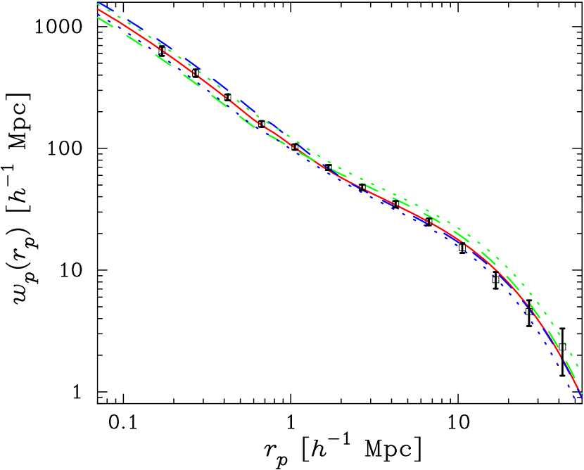
Figure 1.— Shown are the projected correlation function $w_{p}(r_{p})$ of $M_{{}^{0.1}r}<-21$ galaxies from the SDSS LSS sample12 (points with $1\sigma$ diagonal errors) and the best fit three parameter HOD model (solid). Only points with $r<20h^{-1}\rm Mpc$ are used in the fit. Also shown are predicted $w_{p}(r_{p})$ models with $\Omega_{c}$ (dotted) and $\sigma_{8}$ (dashed) at $\pm 3\sigma$ from their best fit values. HOD parameters and other cosmological parameters are held fixed. As seen here, the sensitivity to $\sigma_{8}$ and $\Omega_{c}$ comes from both the amplitude and combined shape of the 1-halo and 2-halo regimes of $w_{p}(r_{p})$.

The observed projected correlation function is obtained from the 2-d correlation function $\xi(r_{p},\pi)$ by integrating along the line of sight in redshift space:

$$w_{p}(r_{p})=2\int_{0}^{\pi_{\rm max}}\xi(r_{p},\pi)d\pi,$$ (11)

where $r_{p}$ and $\pi$ are separations transverse and parallel to the line of sight. We adopt $\pi_{\rm max}=40h^{-1}{\rm Mpc}$ (in the measurement and modeling), large enough to include nearly all correlated pairs and thus minimize redshift-space distortion while keeping background noise from uncorrelated pairs low. Because our sample is volume-limited, we are measuring the clustering of a homogeneous population of galaxies throughout the survey volume, which greatly simplifies HOD modeling. Further details of the sample and measurement are given in Z04b. In our analysis, we use 11 $w_{p}(r_{p})$ data points in the range $0.1h^{-1}{\rm Mpc}<r_{p}<20h^{-1}{\rm Mpc}$, sufficiently below the projection scale $\pi_{\rm max}$ to avoid contamination of redshift space distortions, though we have found that including points up to $r\approx 40h^{-1}\rm Mpc$, which have low statistical weight, does not alter our results.

We also require our models to reproduce the measured mean comoving space density of our sample, $\bar{n}_{g}^{\rm obs}=1.17\times 10^{-3}h^{3}{\rm Mpc}^{-3}$. This quantity has an uncertainty due to sample variance that can be written as $\sigma_{\bar{n}}/\bar{n}_{g}^{\rm obs}=\sqrt{\left<\delta^{2}_{g}\right>}$, where $\left<\delta^{2}_{g}\right>$ is the variance of the galaxy overdensity. We estimate $\left<\delta^{2}_{g}\right>$ by integrating the two-point correlation function over the volume of the SDSS $M_{{}^{0.1}r}<-21$ sample. To compute this integral we generate a large number of independent random pairs of points within the sample volume and sum $\xi(r)$ over all these pairs. We use the Z04b correlation function and extend it to larger scales with the linear theory correlation function multiplied by $b^{2}$, where $b=1.4$ is the large-scale bias factor for $M_{{}^{0.1}r}<-21$ galaxies. We vary the number of random pairs used and find that the integral converges at $10^{5}$ pairs. Using two million pairs, we find that the number density uncertainty due to sample variance is $\sigma_{\bar{n}}/\bar{n}_{g}^{\rm obs}=0.0377$. There is also a shot noise Poisson uncertainty in the number density that, for this number of galaxies, is $0.0062$. We add these two components in quadrature to obtain a total uncertainty of $\sigma_{\bar{n}}^{\rm tot}/\bar{n}_{g}^{\rm obs}=0.0382$, and therefore

$$\bar{n}_{g}^{\rm obs}=(1.17\pm 0.05)\times 10^{-3}h^{3}{\rm Mpc}^{-3}.$$ (12)

4. Results

Table 1Cosmological plus HOD parameters, marginalized constraints with $68.3\%$ C.L. errors.

Parameter	CMB+$w_{p}(r_{p})$ $3p$+$P_{g}(k)$	CMB+$w_{p}(r_{p})$ $3p$	CMB+$w_{p}(r_{p})$ $4p$	CMB+$w_{p}(r_{p})$ $5p$	CMB+$P_{g}(k)$	CMB
$A$	$0.731^{+0.057}_{-0.053}$	$0.749^{+0.063}_{-0.058}$	$0.768^{+0.074}_{-0.068}$	$0.803^{+0.103}_{-0.093}$	$0.747^{+0.077}_{-0.071}$	$0.79^{+0.15}_{-0.12}$
$n$	$0.947^{+0.017}_{-0.018}$	$0.953^{+0.019}_{-0.019}$	$0.958^{+0.020}_{-0.021}$	$0.968^{+0.027}_{-0.027}$	$0.956^{+0.020}_{-0.021}$	$0.974^{+0.037}_{-0.036}$
$\tau$	$0.100^{+0.017}_{-0.021}$	$0.115^{+0.019}_{-0.023}$	$0.131^{+0.021}_{-0.027}$	$0.155^{+0.026}_{-0.037}$	$0.105^{+0.017}_{-0.028}$	$0.158^{+0.093}_{-0.084}$
$h$	$0.687^{+0.023}_{-0.023}$	$0.698^{+0.026}_{-0.026}$	$0.708^{+0.028}_{-0.029}$	$0.721^{+0.034}_{-0.036}$	$0.697^{+0.028}_{-0.028}$	$0.755^{+0.059}_{-0.058}$
$\Omega_{c}h^{2}$	$0.1148^{+0.0039}_{-0.0039}$	$0.1126^{+0.0043}_{-0.0044}$	$0.1107^{+0.0050}_{-0.0049}$	$0.1088^{+0.0058}_{-0.0057}$	$0.1176^{+0.0069}_{-0.0069}$	$0.104^{+0.013}_{-0.013}$
$\Omega_{b}h^{2}$	$0.02234^{+0.00079}_{-0.00080}$	$0.02247^{+0.00084}_{-0.00084}$	$0.02263^{+0.00086}_{-0.00087}$	$0.0229^{+0.0010}_{-0.0010}$	$0.0227^{+0.0009}_{-0.0009}$	$0.0230^{+0.0013}_{-0.0013}$
$M_{1}[10^{13}h^{-1}M_{\odot}]$	$4.79^{+0.63}_{-0.63}$	$4.58^{+0.60}_{-0.60}$	$4.52^{+0.63}_{-0.63}$	$3.31^{+1.61}_{-1.64}$	$-$	$-$
$M_{\rm min}[10^{12}h^{-1}M_{\odot}]$	$3.23^{+0.36}_{-0.35}$	$3.03^{+0.36}_{-0.36}$	$3.26^{+0.46}_{-0.48}$	$3.08^{+0.49}_{-0.51}$	$-$	$-$
$\kappa$	$4.44^{+0.48}_{-0.63}$	$4.44^{+0.51}_{-0.69}$	$3.85^{+0.45}_{-0.56}$	$6.31^{+1.33}_{-1.94}$	$-$	$-$
$\sigma_{\rm cen}$	$0$	$0$	$0.41^{+0.11}_{-0.18}$	$0.39^{+0.10}_{-0.18}$	$-$	$-$
$\alpha$	$1$	$1$	$1$	$0.83^{+0.22}_{-0.23}$	$-$	$-$
$b_{g}$∗	$1.48^{+0.088}_{-0.088}$	$1.47^{+0.093}_{-0.093}$	$1.43^{+0.077}_{-0.077}$	$1.40^{+0.095}_{-0.095}$	$-$	$-$
$\Omega_{m}$	$0.292^{+0.025}_{-0.024}$	$0.278^{+0.027}_{-0.027}$	$0.268^{+0.029}_{-0.029}$	$0.256^{+0.034}_{-0.033}$	$0.291^{+0.034}_{-0.034}$	$0.231^{+0.054}_{-0.056}$
$\sigma_{8}$	$0.809^{+0.028}_{-0.028}$	$0.812^{+0.028}_{-0.027}$	$0.816^{+0.030}_{-0.030}$	$0.829^{+0.039}_{-0.039}$	$0.834^{+0.049}_{-0.050}$	$0.802^{+0.072}_{-0.073}$
$\chi^{2}_{\rm eff}/\rm DOF$	$1483.4/1391$	$1458.5/1373$	$1458.4/1372$	$1458.1/1371$	$1477.2/1383$	$1452.5/1365$
AIC	$1503.4$	$1476.5$	$1478.4$	$1480.1$	$1491.2$	$1464.5$
BIC	$1555.9$	$1523.5$	$1530.7$	$1537.7$	$1527.9$	$1495.8$

Note. — ^∗The large scale galaxy bias ($k\rightarrow 0$).

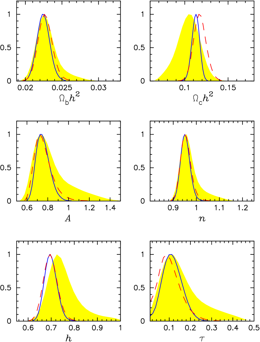
Figure 2.— Shown are the marginalized posterior likelihoods for the cosmological parameters determined from CMB+$w_{p}(r_{p})[M_{{}^{0.1}r}<-21]$ with a three-parameter HOD in solid blue, that for CMB+SDSS 3D $P_{g}(k)$ in red dashed, and that for the CMB alone in yellow (gray) shaded.

For a given cosmology and HOD parameter choice, we use the predicted $w_{p}(r_{p})$ to calculate the likelihood to observe the $M_{{}^{0.1}r}<-21$ sample’s $w_{p}(r_{p})$ and $\bar{n}_{g}^{\rm obs}$. We combine this likelihood with that for the model’s prediction for the cosmic microwave background anisotropy temperature correlation and temperature-polarization cross-correlation to produce the WMAP (first year), ACBAR ($\ell>800$), CBI ($600<\ell<2000$) and VSA ($\ell>600$) observations (Hinshaw et al. 2003; Verde et al. 2003; Kogut et al. 2003; Dickinson et al. 2004; Readhead et al. 2004). We vary the six parameters for the “vanilla” $\Lambda$CDM cosmological model plus the five HOD parameters: $\mathbf{p}=(\Omega_{b}h^{2},\Omega_{c}h^{2},\Theta_{s},\ln(A),n,\tau,M_{\rm min},M_{1},\kappa,\sigma_{\rm cen},\alpha)$. The ranges allowed in our Markov Chain Monte Carlo (MCMC) sampling of parameters are chosen to avoid any artificial cut-off of the likelihood space and are

$$0.005\leq \Omega_{b}h^{2} \leq 0.1$$ (13)

$$0.01\leq \Omega_{c}h^{2} \leq 0.99$$ (14)

$$0.005\leq \Theta_{s} \leq 0.1$$ (15)

$$-0.68\leq \ln(A) \leq 0.62$$ (16)

$$0.5\leq n \leq 1.5$$ (17)

$$0.01\leq \tau \leq 0.8$$ (18)

$$10^{9}\,M_{\odot}\leq M_{\rm min} \leq 5\times 10^{13}\,M_{\odot}$$ (19)

$$10^{10}\,M_{\odot}\leq M_{1} \leq 4\times 10^{14}\,M_{\odot}$$ (20)

$$1\leq \kappa \leq 30$$ (21)

$$0\leq \sigma_{\rm cen} \leq 10$$ (22)

$$0.2\leq \alpha \leq 2.5\;.$$ (23)

Here, $A$ is related to the amplitude of curvature fluctuations at horizon crossing, $|\Delta R|^{2}=2.95\times 10^{-9}A$ at the scale $k=0.05\rm\,Mpc$. The angular acoustic peak scale $\Theta_{s}$ is the ratio of the sound horizon at last scattering to that of the angular diameter distance to the surface of last scattering (Kosowsky et al., 2002).

To measure the likelihood space allowed by the data, we use a Metropolis MCMC method with a modified version of the Lewis & Bridle (2002) CosmoMC code. We use the WMAP team’s code to calculate the WMAP first-year observations’ likelihood, and CosmoMC to calculate that for ACBAR, CBI and VSA. After burn-in, the chains typically sample $10^{5}$ points, and convergence and likelihood statistics are calculated from these. Since it is not known a priori which HOD parameters are most constrained by the $w_{p}(r_{p})$ measurement, we use the Akaike and Bayesian Information Criteria (AIC and BIC) to determine which parameters are statistically relevant to describing $w_{p}(r_{p})$ (Akaike 1974; Schwarz 1978; see also Liddle 2004). More parameters might well be needed once we have more data to constrain the HOD, but $w_{p}(r_{p})$ alone doesn’t provide enough information to demand it.

Likelihood analyses were performed for several cases where some parameters were kept free and others were fixed to a physical limit, i.e. where the scatter in the mass-luminosity relation is unimportant ($\sigma_{\rm cen}\equiv 0$), the cut-off scale of the satellite galaxies is exactly that of the minimum mass $M_{\rm min}$ ($\kappa\equiv 1$), or to a value ($\alpha\equiv 1$) predicted in the numerical simulations and semi-analytic models of satellite halo distributions in Berlind et al. (2003) and Kravtsov et al. (2004). If we adopt all three of these constraints and allow only two parameters, $M_{\rm min}$ and $M_{1}$, to vary to fit $w_{p}(r_{p})$ and $\bar{n}_{g}^{\rm obs}$, then we obtain a poor fit. This model is an inadequate description of the data according to the information criteria ($\Delta{\rm BIC}=7.2$ and $\Delta{\rm AIC}=12.5$) relative to the three-parameter $M_{\rm min}$, $M_{1}$, and $\kappa$ model ($3p$). We also investigated a four parameter model ($4p$), varying $M_{\rm min}$, $M_{1}$, $\kappa$, and $\sigma_{\rm cen}$ with $\alpha\equiv 1$, as well as a five parameter model ($5p$) varying all parameters in this HOD. Relative to the $3p$ model, the $4p$ and $5p$ models introduce new parameters that are not justified by the information criteria ($\Delta{\rm BIC}>6$, cf. Table 1), since these models add freedom but yield only a very small reduction in $\chi^{2}$.

To assess the importance of one aspect of the halo modeling, we performed a test on the $3p$ model whereby the NFW concentration $c_{0}$ [Eq. (7)] of dark matter is replaced by that for the galaxies, $c_{0}^{\rm gal}$, and is also left free in the MCMC within $0.01<c_{0}^{\rm gal}<200$ and independent of the dark matter concentration of the halos. We find that the derived cosmological parameters and their uncertainties remain nearly unchanged from a model with no spatial bias, and the constraints on the galaxy concentration are consistent with no spatial bias: $c_{0}^{\rm gal}=11.1^{+0.7}_{-5.3}$. The marginalized values of the HOD parameters $M_{\rm min}$ and $M_{1}$ remain unchanged with varying $c_{0}^{\rm gal}$, though the error on the cut-off scale of the satellite galaxies $\kappa$ increases ($\kappa=4.71^{+0.60}_{-1.41}$). This increase is expected since it is precisely the central distribution of satellite galaxies that is positively correlated to the one-halo galaxy distribution concentration, with a correlation coefficient of $r=0.72$. As a large $c_{0}^{\rm gal}$ makes the distribution of galaxies inside halos more concentrated, to maintain the small-scale clustering, $\kappa$ increases to allow relatively more galaxies to be put in halos with larger virial radii and lower concentrations.

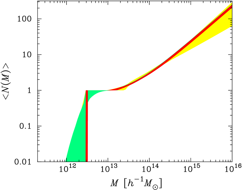
Figure 3.— Plotted are the $\Delta\chi^{2}<1$ range from the best fit for the HOD drawn from the MCMC chains for the $3p$ model in red (dark gray), $4p$ model in green (medium gray), and $5p$ model in yellow (light gray).

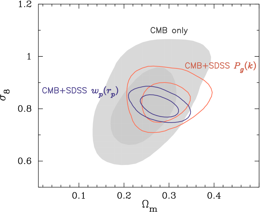
Figure 4.— Shown are the marginalized 68.3% and 95.4% C.L. contours in $\sigma_{8}$ vs. $\Omega_{m}$ for the WMAP+ACBAR+CBI+VSA (CMB) data alone (gray shaded), from the CMB + SDSS 3D $P_{g}(k)$ (orange/light-gray lines) and CMB + SDSS $w_{p}(r_{p})$ (blue/dark-gray lines) from the $3p$ HOD analysis presented here.

Figure 1 illustrates the way that $w_{p}(r_{p})$ constrains cosmological parameters. Data points show the Z04b measurements, and the solid line shows the prediction of the best-fit $3p$ model. Dashed curves show the prediction of the $w_{p}(r_{p})$ after $\sigma_{8}$ is perturbed by $\pm 3\sigma$ relative to its best-fit value given in column 2 of Table 1, with all other cosmological parameters (and therefore the shape of the linear matter power spectrum) as well as the HOD parameters held fixed. Dotted curves show the prediction of $w_{p}(r_{p})$ after changing $\Omega_{c}$, and thus the shape of the transfer function in the matter power spectrum, by $\pm 3\sigma$, with all other cosmological and HOD parameters fixed. The strength of the constraints derived from $w_{p}(r_{p})$ stems from the combined relative dependence of the 1-halo and 2-halo regimes and therefore the overall shape of $w_{p}(r_{p})$.

The cosmological parameters’ marginalized posterior likelihoods for the $3p$ model are shown in Figure 2. Also shown for comparison are the marginalized likelihoods for the CMB plus SDSS 3D $P_{g}(k)$ [updated from Tegmark et al. (2004) with new CMB results], and that from the CMB data alone. We also combine the CMB+$w_{p}(r_{p})(3p)$ measurement with the SDSS 3D $P_{g}(k)$ for a joint constraint on cosmological parameters. Since the $P_{g}(k)$ data points included in the analysis are at wavelengths $\lambda=2\pi/k>30\,h^{-1}\,{\rm Mpc}$, the information they contain is largely independent of that in the $w_{p}(r_{p})$ data points at $r_{p}<20\,h^{-1}\,{\rm Mpc}$. All parameters’ best fit values and errors are listed in Table 1. The resulting range of the HOD measured for all models here are shown in Figure 3.

Two-dimensional contours of $\Omega_{m}$ and $\sigma_{8}$ are shown in Figure 4 and are compared to those obtained using CMB alone or CMB + $P_{g}(k)$. The anticorrelation of $\Omega_{m}$ and $\sigma_{8}$ from the $w_{p}(r_{p})$ constraint seen in Fig. 4 arises from the anticorrelated degeneracy in these parameters in the one-halo component due to its dependence on the halo mass function which needs to maintain its amplitude at high halo masses, and the $Omega_{m}$ and $\sigma_{8}$ anticorrelation in the two-halo component due to the amplitude-shape degeneracy of the dark matter power spectrum (or dark matter correlation function).

Important results to note from the Figures and Table are the following. Cosmological constraints obtained using CMB and $w_{p}(r_{p})$ are substantially tighter than those from CMB alone, and they are similar in value and tightness to those obtained from CMB + $P_{g}(k)$ despite the introduction of new parameters to represent the HOD. The $\sigma_{8}$ constraints using $w_{p}(r_{p})$ are tighter than those using $P_{g}(k)$; note that the latter estimate has dropped relative to that of Tegmark et al. (2004) because of the smaller scale CMB data. If we incorporate $P_{g}(k)$ constraints in addition to $w_{p}(r_{p})$, then parameter values change by less than $1-\sigma$ and error bars improve slightly. Our cosmological parameter results also agree, within errors, with the recent results from SDSS galaxy bias and Lyman-$\alpha$ forest (Seljak et al., 2004b). The HOD parameters are partially degenerate among themselves, so adding parameters to the HOD model worsens the constraint on any one of them. However, within the range of models examined here, adding parameters to the HOD only slightly increases the error bars on cosmological parameters.

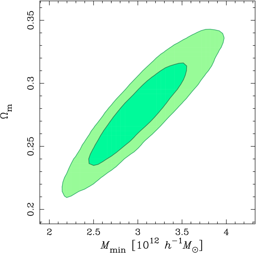
Figure 5.— Plotted are the 68.3% and 95.4% C.L. contours for the marginalized likelihoods for $\Omega_{m}$ vs. $M_{\rm min}$. The strong degeneracy (correlation of $r=0.92$) roughly follows $\Omega_{m}\propto M_{\rm min}$, as expected (Zheng et al., 2002; Rozo et al., 2004)

Since the small scales of the primordial power spectrum probed by $w_{p}(r_{p})$ could be useful in constraining any deviations from a simple power-law primordial spectrum as well as a model including the suppression in power spectrum and mass function due to the presence of massive neutrinos, we performed an MCMC analysis including a running of the spectrum $dn/d\ln k$ about the scale $k=0.05\rm\;Mpc$ for the $3p$ HOD model as well a model including massive neutrinos. We find little evidence for running, $dn/d\ln k=-0.062^{+0.026}_{-0.027}$, comparable to the results of Spergel et al. (2003). The halo model in the presence of massive neutrinos is applied such that the halo mass function, halo bias and halo profile is that of the cold dark matter alone since neutrino clustering is a very small effect on these quantities (Abazajian et al., 2004a). The presence of massive neutrinos is constrained to $m_{\nu}<0.27\rm\,eV$ ($95\%$ C.L.) for each of 3 neutrinos with degenerate mass. The statistical errors from our analysis of the CMB plus this $w_{p}(r_{p})$ measurement on $dn/d\ln k$ and $m_{\nu}$ are comparable to those from other cosmological parameter analyses, being smaller than those from the shape of the SDSS 3D $P_{g}(k)$ plus WMAP (Tegmark et al., 2004), comparable to the WMAP plus 2dFGRS 3D $P_{g}(k)$ plus modeled bias constraints (Spergel et al., 2003), but not as stringent as those from modeling the galaxy bias in the SDSS from galaxy-galaxy lensing and clustering of the Lyman-$\alpha$ forest in the SDSS (Seljak et al., 2004a, b).

5. Discussion

The remaining uncertainties in cosmological parameters introduce relatively little uncertainty in the HOD parameters, i.e., we now know the underlying cosmology with sufficient precision to pin down the relation between galaxies and mass. The strongest expected degeneracy is between the value of $\Omega_{m}$ and the mass scale parameters $M_{\rm min}$ and $M_{1}$, since one can compensate a uniform increase in halo masses by simply shifting galaxies into more massive halos (Zheng et al., 2002; Rozo et al., 2004). The error contours for $\Omega_{m}$ vs. $M_{\rm min}$ are shown in Figure 5. The degeneracy between these parameters is strong, with a correlation of $r=0.96$. While this degeneracy would cause large uncertainties in the values of $M_{\rm min}$ and $\Omega_{m}$ if we used the galaxy clustering data alone, the combination of CMB and $w_{p}(r_{p})$ data constrains $\Omega_{m}$ fairly tightly, leaving limited room to vary the mass scale parameters. Incorporating SDSS clustering measures that are directly sensitive to halo masses, such as redshift-space distortions (Zehavi et al., 2002) and galaxy-galaxy lensing measurements (Sheldon et al., 2004; Seljak et al., 2004a), may further improve the $\Omega_{m}$ constraints.

As discussed by Berlind & Weinberg (2002), the galaxy correlation function places important constraints on HOD parameters, but it still allows tradeoffs between different features of $P(N|M)$ and (to a lesser degree) between $P(N|M)$ and the assumed spatial bias of galaxies within halos. Additional clustering statistics such as the group multiplicity function, higher order correlation functions, and void probabilities impose complementary constraints that can break these degeneracies. Our analysis should thus be seen as a first step in a broader program of combining galaxy clustering measurements from the SDSS and other surveys with other cosmological observables to derive simultaneous constraints on cosmological parameters and the galaxy HOD [see Berlind & Weinberg (2002); Weinberg (2002); Zheng et al. (2002) for further discussion]. Van den Bosch et al. (2003) have been carrying out a similar program using the closely related conditional luminosity function (CLF) method applied to the 2dFGRS luminosity and correlation functions (see also van den Bosch et al. 2004). They find $\sigma_{8}=0.78\pm 0.12$ and $\Omega_{m}=0.25^{+0.10}_{-0.07}$ in their analysis combined with CMB data, with both errors at $95\%$ C.L. as given in that work. Our results are in agreement, within errors, with their determinations of $\sigma_{8}$ and $\Omega_{m}$.

Besides the statistical error bars, there are two main sources of systematic uncertainty in our cosmological parameter estimates. The first is the possibility that our HOD parameterization does not have enough freedom to describe the real galaxy HOD, and that we are artificially shrinking the cosmological error bars by adopting a restrictive theoretical prior in our galaxy bias model. For the $3p$ model, this is arguably the case, since it effectively assumes perfect correlation between the mass of a halo and the luminosity of its central galaxy. However, our $5p$ model is able to give an essentially perfect description of the predictions of semi-analytic galaxy formation models and hydrodynamic simulations (Zheng 2004; see also Guzik & Seljak 2002; Berlind et al. 2003; Kravtsov et al. 2004), so there is good reason to think that the error bars quoted for this case are conservative. This model still makes the assumption that satellite galaxies have no spatial bias with respect to dark matter within halos, but the concentration test in §4 shows that dropping this assumption has minimal impact on cosmological conclusions. In place of an HOD model, traditional analyses based on the large-scale galaxy power spectrum assume that the galaxy power spectrum is a scale-independent multiple of the linear matter power spectrum, so that their shapes are identical. Scale-independence in the linear regime is expected on fairly general grounds (Coles, 1993; Fry & Gaztanaga, 1993; Weinberg, 1995; Mann et al., 1998; Scherrer & Weinberg, 1998; Narayanan et al., 2000). However, it is not clear just how well this approximation holds over the full range of scales used in the power spectrum analyses, so although our HOD models are considerably more complex than linear bias models, our approach is arguably no more dependent on theoretical priors. In future work, we can use the HOD modeling to calculate any expected scale-dependence of the power spectrum bias, thus improving the accuracy of the power spectrum analyses and allowing them to extend to smaller scales.

The second source of systematic uncertainty is the possibility that our approximation for calculating $w_{p}(r_{p})$ for a given cosmology and HOD is inaccurate in some regions of our parameter space. The ingredients of this approximation have been calibrated or tested on N-body simulations of cosmological models similar to the best fitting models found here, so we do not expect large inaccuracies. However, there are several elements of the halo model calculation that could be inaccurate or cosmology dependent at the 10% level that is now of interest, including departures from the Jenkins et al. (2001) mass function, scale dependence of halo bias, and details of halo exclusion. Uncertainties in the halo mass-concentration relation and the impact of scatter in halo concentrations come in at a similar level, though the test in §4 again indicates that these uncertainties mainly affect the details of the derived HOD, not the cosmological parameter determinations. Without a comprehensive numerical study of these issues, it is difficult to assess how large the systematic effects on our parameter determinations could be, but we would not be surprised to find that they are comparable to our statistical errors. We plan to carry out such a study to remove this source of systematic uncertainty in future work; the papers of Seljak & Warren (2004) and Tinker et al. (2004) present steps along this path.

Analyses of multiple classes of galaxies will allow consistency checks on any cosmological conclusions, since different classes will have different HODs but should yield consistent cosmological constraints. By drawing on the full range of galaxy clustering measurements, joint studies of galaxy bias and cosmological parameters will sharpen our tests of the leading theories of galaxy formation and the leading cosmological model. With this current analysis alone, we find that the combination of CMB anisotropies and small-scale galaxy clustering measurements provides, simultaneously, tight constraints on the occupation statstics of galaxies in dark matter halos, and some of the best available constraints on fundamental cosmological parameters.

References

- Abazajian et al. (2004a) Abazajian, K., Switzer, E. R., Dodelson, S., Heitmann, K., & Habib, S. 2004a, Phys. Rev. D submitted, astro-ph/0411552
- Abazajian et al. (2003) Abazajian, K. et al. 2003, AJ, 126, 2081
- Abazajian et al. (2004b) —. 2004b, AJ, 128, 502
- Akaike (1974) Akaike, H. 1974, IEEE Trans. Auto. Control, 19, 716
- Benson et al. (2000) Benson, A. J., Cole, S., Frenk, C. S., Baugh, C. M., & Lacey, C. G. 2000, MNRAS, 311, 793
- Berlind & Weinberg (2002) Berlind, A. A. & Weinberg, D. H. 2002, ApJ, 575, 587
- Berlind et al. (2003) Berlind, A. A. et al. 2003, ApJ, 593, 1
- Blanton et al. (2003a) Blanton, M. R., Brinkmann, J., Csabai, I., Doi, M., Eisenstein, D., Fukugita, M., Gunn, J. E., Hogg, D. W., & Schlegel, D. J. 2003a, AJ, 125, 2348
- Blanton et al. (2004a) Blanton, M. R., Eisenstein, D. J., Hogg, D. W., & Zehavi, I. 2004a, ApJ submitted, astro-ph/0411037
- Blanton et al. (2003b) Blanton, M. R., Lin, H., Lupton, R. H., Maley, F. M., Young, N., Zehavi, I., & Loveday, J. 2003b, AJ, 125, 2276
- Blanton et al. (2004b) Blanton, M. R. et al. 2004b, AJ submitted, astro-ph/0410166
- Bryan & Norman (1998) Bryan, G. L. & Norman, M. L. 1998, ApJ, 495, 80
- Coles (1993) Coles, P. 1993, MNRAS, 262, 1065
- Colless et al. (2003) Colless, M. et al. 2003, astro-ph/0306581
- Cooray & Sheth (2002) Cooray, A. & Sheth, R. 2002, Phys. Rept., 372, 1
- Dickinson et al. (2004) Dickinson, C. et al. 2004, MNRAS, 353, 732
- Eisenstein et al. (2001) Eisenstein, D. J. et al. 2001, AJ, 122, 2267
- Fry & Gaztanaga (1993) Fry, J. N. & Gaztanaga, E. 1993, ApJ, 413, 447
- Fukugita et al. (1996) Fukugita, M. et al. 1996, AJ, 111, 1748
- Gunn et al. (1998) Gunn, J. E. et al. 1998, AJ, 116, 3040
- Guzik & Seljak (2002) Guzik, J. & Seljak, U. 2002, MNRAS, 335, 311
- Hinshaw et al. (2003) Hinshaw, G. et al. 2003, ApJS, 148, 135
- Hogg et al. (2001) Hogg, D. W., Finkbeiner, D. P., Schlegel, D. J., & Gunn, J. E. 2001, AJ, 122, 2129
- Hu & Kravtsov (2003) Hu, W. & Kravtsov, A. V. 2003, ApJ, 584, 702
- Huffenberger & Seljak (2003) Huffenberger, K. M. & Seljak, U. 2003, MNRAS, 340, 1199
- Jenkins et al. (2001) Jenkins, A. et al. 2001, MNRAS, 321, 372
- Jing et al. (2002) Jing, Y. P., Börner, G., & Suto, Y. 2002, ApJ, 564, 15
- Jing et al. (1998) Jing, Y. P., Mo, H. J., & Boerner, G. 1998, ApJ, 494, 1
- Kauffmann et al. (1999) Kauffmann, G., Colberg, J. M., Diaferio, A., & White, S. D. M. 1999, MNRAS, 303, 188
- Kauffmann et al. (1997) Kauffmann, G., Nusser, A., & Steinmetz, M. 1997, MNRAS, 286, 795
- Kogut et al. (2003) Kogut, A. et al. 2003, ApJS, 148, 161
- Kosowsky et al. (2002) Kosowsky, A., Milosavljevic, M., & Jimenez, R. 2002, Phys. Rev., D66, 063007
- Kravtsov et al. (2004) Kravtsov, A. V., Berlind, A. A., Wechsler, R. H., Klypin, A. A., Gottlöber, S., Allgood, B., & Primack, J. R. 2004, ApJ, 609, 35
- Lewis & Bridle (2002) Lewis, A. & Bridle, S. 2002, Phys. Rev., D66, 103511
- Lewis et al. (2000) Lewis, A., Challinor, A., & Lasenby, A. 2000, ApJ, 538, 473
- Liddle (2004) Liddle, A. R. 2004, MNRAS, 351, L49
- Magliocchetti & Porciani (2003) Magliocchetti, M. & Porciani, C. 2003, MNRAS, 346, 186
- Mann et al. (1998) Mann, R. G., Peacock, J. A., & Heavens, A. F. 1998, MNRAS, 293, 209
- Narayanan et al. (2000) Narayanan, V. K., Berlind, A. A., & Weinberg, D. H. 2000, ApJ, 528, 1
- Navarro et al. (1996) Navarro, J. F., Frenk, C. S., & White, S. D. M. 1996, ApJ, 462, 563
- Peacock & Smith (2000) Peacock, J. A. & Smith, R. E. 2000, MNRAS, 318, 1144
- Percival et al. (2001) Percival, W. J. et al. 2001, MNRAS, 327, 1297
- Pier et al. (2003) Pier, J. R. et al. 2003, AJ, 125, 1559
- Porciani & Giavalisco (2002) Porciani, C. & Giavalisco, M. 2002, ApJ, 565, 24
- Porciani et al. (2004) Porciani, C., Magliocchetti, M., & Norberg, P. 2004, MNRAS, 539
- Readhead et al. (2004) Readhead, A. C. S. et al. 2004, ApJ, 609, 498
- Richards et al. (2002) Richards, G. T. et al. 2002, AJ, 123, 2945
- Rozo et al. (2004) Rozo, E., Dodelson, S., & Frieman, J. A. 2004, Phys. Rev., D70, 083008
- Scherrer & Weinberg (1998) Scherrer, R. J. & Weinberg, D. H. 1998, ApJ, 504, 607
- Schwarz (1978) Schwarz, G. 1978, Annals of Statist., 5, 461
- Scoccimarro et al. (2001) Scoccimarro, R., Sheth, R. K., Hui, L., & Jain, B. 2001, ApJ, 546, 20
- Seljak (2000) Seljak, U. 2000, MNRAS, 318, 203
- Seljak & Warren (2004) Seljak, U. & Warren, M. S. 2004, MNRAS, 516
- Seljak & Zaldarriaga (1996) Seljak, U. & Zaldarriaga, M. 1996, ApJ, 469, 437
- Seljak et al. (2004a) Seljak, U. et al. 2004a, Phys. Rev. D submitted, astro-ph/0406594
- Seljak et al. (2004b) —. 2004b, Phys. Rev. D submitted, astro-ph/0407372
- Sheldon et al. (2004) Sheldon, E. S. et al. 2004, AJ, 127, 2544
- Sheth et al. (2001) Sheth, R. K., Mo, H. J., & Tormen, G. 2001, MNRAS, 323, 1
- Sheth & Tormen (1999) Sheth, R. K. & Tormen, G. 1999, MNRAS, 308, 119
- Smith et al. (2002) Smith, J. A. et al. 2002, AJ, 123, 2121
- Somerville et al. (2001) Somerville, R. S., Lemson, G., Sigad, Y., Dekel, A., Kauffmann, G., & White, S. D. M. 2001, MNRAS, 320, 289
- Spergel et al. (2003) Spergel, D. N. et al. 2003, ApJS, 148, 175
- Stoughton et al. (2002) Stoughton, C. et al. 2002, AJ, 123, 485
- Strauss et al. (2002) Strauss, M. A. et al. 2002, AJ, 124, 1810
- Takada & Jain (2003) Takada, M. & Jain, B. 2003, MNRAS, 340, 580
- Tegmark et al. (2004) Tegmark, M. et al. 2004, Phys. Rev., D69, 103501
- Tinker et al. (2004) Tinker, J. L., Weinberg, D. H., Zheng, Z., & Zehavi, I. 2004, ApJ submitted, astro-ph/0411777
- Van den Bosch et al. (2003) Van den Bosch, F. C., Mo, H. J., & Yang, X. 2003, MNRAS, 345, 923
- van den Bosch et al. (2004) van den Bosch, F. C., Mo, H. J., & Yang, X. 2004, MNRAS, 348, 736
- Verde et al. (2003) Verde, L. et al. 2003, ApJS, 148, 195
- Wang et al. (2004) Wang, Y., Yang, X.-H., Mo, H. J., van den Bosch, F. C., & Chu, Y.-Q. 2004, Mon. Not. Roy. Astron. Soc., 353, 287
- Weinberg (1995) Weinberg, D. H. 1995, in Wide-Field Spectroscopy and the Distant Universe, ed. S. J. Maddox & A. Aragón-Salamanca (Singapore: World Scientific), 129, astro–ph/9409094
- Weinberg (2002) Weinberg, D. H. 2002, in A New Era in Cosmology, ed. T. Shanks & N. Metcalfe (San Francisco: ASP Conference Series), 3, astro–ph/0202184
- White (2001) White, M. 2001, A&A, 367, 27
- White et al. (2001) White, M., Hernquist, L., & Springel, V. 2001, ApJ, 550, L129
- York et al. (2000) York, D. G. et al. 2000, AJ, 120, 1579
- Zehavi et al. (2002) Zehavi, I. et al. 2002, ApJ, 571, 172
- Zehavi et al. (2004a) —. 2004a, ApJ, 608, 16
- Zehavi et al. (2004b) —. 2004b, ApJ submitted, astro-ph/0408569
- Zheng (2004) Zheng, Z. 2004, ApJ, 610, 61
- Zheng et al. (2002) Zheng, Z., Tinker, J. L., Weinberg, D. H., & Berlind, A. A. 2002, ApJ, 575, 617
- Zheng et al. (2004) Zheng, Z. et al. 2004, ApJ submitted, astro-ph/0408564