$K$–band Properties of Well-Sampled Groups of Galaxies

Abstract

We use a sample of 55 groups and 6 clusters of galaxies ranging in mass from 7 $\times$10${}^{11}M_{\odot}$ to 1.5 $\times$10${}^{15}M_{\odot}$ to examine the correlation of the $K_{s}$–band luminosity with mass discovered by Lin et al. (2003). We use the 2MASS catalog and published redshifts to construct complete magnitude limited redshift surveys of the groups. From these surveys we explore the IR photometric properties of groups members including their IR color distribution and luminosity function. Although we find no significant difference between the group $K_{s}$ luminosity function and the general field, there is a difference between the color distribution of luminous group members and their counterparts (generally background) in the field. There is a significant population of luminous galaxies with (H-$K_{s}$) $\gtrsim$ 0.35 which are rarely, if ever, members of the groups in our sample. The most luminous galaxies which populate the groups have a very narrow range of IR color. Over the entire mass range covered by our sample, the $K_{s}$ luminosity increases with mass as $L_{K_{s}}\propto M^{0.64\pm 0.06}$ implying that the mass-to-light ratio in the $K_{s}$–band increases with mass. The agreement between this result and earlier investigations of essentially non-overlapping sets of systems shows that this window in galaxy formation and evolution is insensitive to the selection of the systems and to the details of the mass and luminosity computations.

1 Introduction

In the low redshift universe, most galaxies reside in groups (Gott and Turner 1977; Gregory and Thompson 1978; Faber and Gallagher 1979; Huchra & Geller 1982; Ramella et al. 1997; Ramella et al. 1999). Thus, in spite of the difficulty of determining the dynamical and photometric properties of these often sparse systems, they have served as a measure of the universal mass-to-light ratio (Faber & Gallagher 1979; Ramella et al. 1997; Tucker et al. 2000; Bahcall et al. 2000; Carlberg et al. 2001).

Early studies of groups of galaxies are based primarily on surveys drawn from the Zwicky catalog (Zwicky et al. 1961-1968). Problems including the small number of observed members, the membership assignment itself, and non-uniform photometry led to a large spread in group mass-to-light ratios even if the median was robust to the myriad observational problems. Groups thus provided one of the routes to an estimate of the universal mean cosmological mass density, $\Omega_{m}$. Because both the systematic and internal random errors in mass-to-light ratio determination were large, there was little consideration of either the presence or the impact of group (cluster) mass-to-light ratios that vary with mass.

As both photometric and redshift surveys have increased in size and quality, refined analyses of the data have revealed a potential dependence of the mass-to-light ratio of systems on the system mass and/or velocity dispersion. Girardi et al. (2000) and later Girardi et al. (2002) used heterogeneous data to demonstrate a dependence of blue mass-to-light ratio on mass, $M/L_{B}\propto M^{0.17-0.23}$. Bahcall & Comerford (2002) derive an analogous dependence of $M/L_{B}$ on X–ray temperature which they attribute to differences in the ages of the stellar population for galaxies in groups of different mass. The decrease in the fraction of star-forming galaxies with the mass or velocity dispersion of groups appeared to support the argument that the variation in mass-to-light ratio with mass was a population effect (see e.g. Biviano et al. 1997; Koranyi & Geller 2002; Balogh et al. 2004).

Recent analyses by Lin et al. (2003 (L03 hereafter), 2004 (L04 hereafter)) of systems of galaxies based on X–ray data for mass determination and Two-Micron All-Sky Survey (2MASS, Jarrett et al. 2000) data for luminosity determination suggest a profoundly different interpretation of the mass dependence of group mass-to-light ratios. L03 show that $M/L_{K_{s}}\propto M^{0.31\pm 0.09}$, steeper than, but consistent with, the earlier B-band relations. Rines et al. (2004) find a similar dependence of $K_{s}$ mass-to-light ratio on system mass and/or velocity dispersion in their study of nine very well-observed clusters of galaxies. Their mass estimates depend on the dynamics of the cluster galaxy population.

The variation in infrared color with changes in stellar population is much smaller than the analogous variation in optical bands. Thus, if the mass dependence were a population effect, one would expect a shallower $K_{s}$ relation. L03 and L04 suggest that the dependence of $K_{s}$ mass-to-light ratio on mass provides a new window on the galaxy formation process. They suggest that the dependence results from lower efficiency and/or efficient disruption of galaxies in massive systems.

In contrast with L03, L04 and Rines et al. (2004), Kochanek et al. (2003) use 2MASS data to argue that mass-to-light ratios are essentially independent of system mass, consistent with the historical perception that the mass-to-light ratios of groups are roughly independent of the mass of the system. The explanation of the difference between the L03, L04 and Kochanek et al. (2003) results is unclear, but the approaches they take to the the problem are very different. L03 and L04 analyze sets of systems well-observed in the X–ray. Kochanek et al. (2001) use N-body simulations to guide their broad statistical analysis based on a matched filter algorithm. They use dynamical methods and calibration to X–ray data to estimate masses.

Here we take an approach in between that of L03, L04, and Kochanek et al. (2003) to investigate the dependence of $K_{s}$–band mass-to-light ratios on the mass of the system. We compile a set of systems initially selected from a complete redshift survey with subsequent deeper spectroscopic surveys (Mahdavi et al. 1999; Mahdavi & Geller 2004). Most of these systems (but not all) have associated extended X–ray emission (Mahdavi et al. 2000). We use the complete redshift surveys as a basis for mass estimation. We supplement our sample with other optically identified systems to enlarge the sample. The dependence of $K_{s}$–band mass-to-light ratio on mass agrees very well with the results of L03 and L04.

L03 and L04 use statistical background subtraction rather than redshift surveys to assess system membership. We examine this procedure by studying the photometric properties of group members and non-group galaxies. Although we find a substantial color difference between the two populations, we show that this difference does not bias the procedure followed by L03 and L04.

We begin our discussion of the $K_{s}$ properties of groups with a discussion of the group catalog and the construction of a complete magnitude limited redshift list for each group using the 2MASS catalog (Section 2). Section 3 discusses the infrared photometric properties of groups members. Section 3.1 is a discussion of the IR colors of groups members and non-members (generally background). We discuss the $K_{s}$–band luminosity function (LF) of the groups in our sample in Section 3.2. In Section 4 we investigate the dependence of $K_{s}$ light as a function of the mass of the system as determined from the virial theorem. We compare the results of Section 4 with L03, L04, and Rines et al. (2004) in Section 5 and we conclude in Section 6. Throughout this paper we use $H_{0}=100\,h$ km sec^-1 Mpc^-1.

2 The Group Catalog and Group Membership

The 2MASS extended source catalog (Jarrett et al. 2000; 2MASS) provides uniform photometry over the entire sky potentially enabling a uniform comparison of the photometric and dynamical properties of systems of galaxies (Kochanek et al. 2003; L03; L04). To obtain estimates of system mass and $K_{s}$–band luminosity, we compile a set of poor systems which are well-sampled in redshift space.

We select our group and cluster sample from existing catalogs. We use galaxy redshifts in 39 well-sampled groups (Mahdavi et al. 1999; Mahdavi & Geller 2004). These systems constitute our ”core” sample because they were selected and observed in a homogeneous way. Groups in this sample were identified in an unbiased way from complete, magnitude limited redshift-surveys (CfA2 and SSRS2). Subsequently Mahdavi et al. (1999) and Mahdavi & Geller (2004) measured redshifts to a deeper magnitude limit within a projected radius $R_{search}$ = 1.5 $h^{-1}$ Mpc. We supplement this sample with 8 groups from Zabludoff & Mulchaey (1998) and 14 AWM/MKW poor clusters from Koranyi & Geller (2002). Table 1 lists these 61 systems.

These 61 systems are at low redshift (cz $\lesssim$ 12,000 km s^-1 ) and span a three-order-of-magnitude range in mass. Most of our systems have extended X–ray emission, certifying their reliability as physical systems. Thirty (77%) of the Mahdavi et al. (1999, 2004) groups are associated with extended X–ray emission as are 6 (75%) of the Zabludoff & Mulchaey (1998) and 8 (57%) of the Koranyi & Geller (2002) systems. The groups not associated with extended X–ray sources may be below the current detection thresholds.

To obtain an estimate of the group luminosity we use the $K_{s}$–band 20 mag arcsec^-2 isophotal fiducial elliptical aperture magnitudes from 2MASS.

We use thes magnitudes following Jarrett (2003; the FAQ sheet for the 2MASS Extended Source Catalog (http://spider.ipac.caltech.edu/staff/jarrett/2mass/XSC/ jarrett_XSCprimer. html) who emphasizes that ”the isophotal elliptical magnitudes provide accurate colors for galaxies of all sizes” while still ”capturing most of the integrated flux ( 80-90%)”

For each system from Mahdavi et al. (1999) and Mahdavi & Geller (2004), we select all galaxies in the 2MASS extended source catalog (Jarrett et al. 2000) which lie within 1.5 $h^{-1}$ Mpc of the center listed in Table 1. For systems observed by Zabludoff & Mulchaey (1999) and Koranyi & Geller (2002) we search the 2MASS catalog to the radius listed in Table 1.

We match these 2MASS galaxies with the galaxy redshift list for each group. For redshifts from Mahdavi et al. (1999, 2004), Zabludoff & Mulchaey (1999), and Koranyi & Geller (2002) we take the membership assignments given by these authors. We searched NED for additional members of each group. We include additional galaxies as members if the redshift is within 3 $\sigma$ (the velocity dispersion within the limiting search radius in Table 1) of the group mean redshift. This procedure yields 90 additional redshifts including 29 additional members. These last redshifts enable us to extend the completeness limit of each group redshift survey to a fainter limit.

We rank system members according to their $K_{s}$ magnitude and identify the faintest magnitude $K_{s,lim,complete}$ for which the group redshift survey is complete. Because the subsamples $K_{s}$ $\leq$ $K_{s,lim,complete}$ are, in some cases, rather small, we increase the magnitude limit as much as possible by requiring that at most one galaxy without a redshift is included within $K_{s,lim}$. The inclusion of a single galaxy without a measured redshift does produce a substantial gain in the sampling of 39 groups. With this procedure, our individual group surveys reach $\sim$ 0.3 magnitudes fainter and we include a total of 200 (101) additional galaxies (members). In six cases we add more than ten galaxies to individual groups. Our apparent magnitude limits are in the range 10.83 $\leq$ $K_{s,lim,complete}$$\leq$ 13.45, with a large fraction close to $K_{s}$ = 13.0 (median $K_{s,lim,complete}$ = 12.85, with inter-quartile range i.q.r = .22). The corresponding absolute magnitude limits peak at $\sim M_{s,lim,complete}$ = -21.3 with i.q.r. = 0.4.

We assign the mean redshift of the group to the single galaxy without spectroscopy and verify that the inclusion/exclusion of this galaxy from the member list does not alter any of our results significantly. In the analysis below we use the samples limited to $K_{s,lim}$.

The physical quantities we investigate are the mass and total luminosity in the $K_{s}$–band within some fiducial radius. To obtain a physically meaningful and stable estimate of the radius, we use $R_{200}$, the radius enclosing an overdensity 200 $\rho_{crit}(z)$ (Carlberg et al. 1997), where $\rho_{crit}(z)$ the critical density for an Einstein - de Sitter universe at redshift $z$.

Our systems are not rich enough for a reliable fit to a model density profile (e.g. Navarro et al. 1997; NFW). We thus assume that the groups are in virial equilibrium and that their mass increases linearly with the radius, $r$. Under these conditions (Carlberg et al. 1997), $R_{200}=\sqrt{3}\,\sigma(1+z)^{-3/2}/(10\,H_{o})$ where we compute $\sigma$ from all the member galaxies within the limiting search radius (Table 1) irrespective of $K_{s}$ magnitude of the galaxies. This procedure is similar to the one employed by Carlberg et al. (1997) for clusters.

The velocity dispersion profiles of groups of galaxies vary. Mahdavi et al. (1999), Mahdavi & Geller (2004), and Koranyi & Geller (2002) show that the velocity dispersion profiles may be rising, falling or flat. As a result of these variations, there is, in general, a difference between $\sigma$ and $\sigma_{200}$, the velocity dispersion within $R_{200}$. However, the median difference between $\sigma$ and $\sigma_{200}$ is negligible: the median relative difference is 4% with a narrow 4% inter-quartile range. In the worst case (marked “a” in Table 1) the difference is 30%, in few other cases the difference is about 20%, and in all other cases it is much less.

The median $R_{200}$ is $R_{200,median}$ = 0.7 $h^{-1}$ Mpc with an interquartile range of 0.18 $h^{-1}$ Mpc. We compute a virial mass within $R_{200}$: $M_{vir,200}$ = 3 G^-1 $R_{200}$ $\sigma_{200}$². There are five systems with fewer than five members brighter than $K_{s,lim}$ within $R_{200}$. We exclude these systems (marked “b” in Table 1) from further analysis. We also exclude an additional system where $R_{200}$ is one third of its search radius (marked “c” in Table 1). We retain four other groups that have $R_{200}$ slightly larger than their search radius. The total sample we analyze then contains 55 systems; 35 of these systems include a single galaxy without redshift. The final group sample contains a total of 1192 (955) galaxies (members).

3 The Infrared Properties of Group Members

The three IR bands of the 2MASS survey allow investigation of the IR colors and magnitudes of $\sim 1200$ galaxies within the complete redshift surveys of our 55 groups. In Section 3.1 we examine the color distribution of galaxies in groups as a function of absolute magnitude and compare these distributions with the non-members (generally background galaxies).

$K_{s}$–band spectroscopy of nearby star-forming spiral galaxies reveals a $\sim$20% contribution to the $K_{s}$–band luminosity from 1000 K dust (James and Seigar 1999). We thus explore infrared color-color diagrams for the group and “field” galaxies to assess the importance of extinction and/or dust emission as a contributor to the $K_{s}$–band light from galaxy groups.

In Section 3.2 we consider the constraints our group redshift surveys place on the group luminosity and we compare the group luminosity function (GLF) with the LF for the “general field” determined by Kochanek et al. (2001) and Cole et al. (2001).

3.1 The infrared Color Distributions and Color-Color Diagrams

Our sample of 55 groups contains 955 group members and 237 non-member galaxies with magnitudes measured in all three bands, J, H and $K_{s}$, and with $K_{s}$ $\leq$ $K_{s,lim}$. We compute the absolute magnitude in the $K_{s}$–band, $M_{K_{s}}$, and derive the quartiles of the distribution of $M_{K_{s}}$: $Q_{1}$ = -23.60, $Q_{2}$ = -22.76, and $Q_{3}$ = -22.08. To examine the color distributions of members and non-members we separate galaxies into four classes of absolute magnitude ($M_{K_{s}}<Q_{1}$, $Q_{1}\leq M_{K_{s}}<Q_{2}$, $Q_{2}\leq M_{K_{s}}<Q_{3}$, and $M_{K_{s}}\geq Q_{3}$ are intervals I, II, III, and IV respectively). We show below that K-corrections have a negligible effect on these distributions.

The four panels of Figure 1 show histograms of the ($J-K_{s}$) color of member galaxies (solid line) and of the non-members (dot-dashed line) in each absolute magnitude bin (thin line).

The most striking features of the histograms are: a) the very narrow peak of the color histogram of the (intrinsically) brightest member galaxies in panel I (i.q.r. = 0.02), and b) the marked difference between the color distributions of these intrinsically luminous member and non-member galaxies (panel I). The difference between members and non-members is still apparent in panel II but disappears for the intrinsically fainter galaxies in panels III and IV. Low luminosity non-members are rare in these magnitude limited samples. The distribution of colors for the entire sample in each absolute magnitude range (members and non-members) shifts blue-ward for intrinsically less luminous galaxies. This effect is the same as the one observed by Cole et al. (2001) in their analysis of 2MASS properties of galaxies in a sample extracted from the 2dF redshift survey.

Figure 2 shows another view of the narrow peak in the ($J-K_{s}$)  color distribution for members in quartile I as a function of $M_{K_{s}}$. The black dots denote member galaxies; the circles denote the non-members. The symbol size is proportional to the redshift of the group. Inspection of the Second STScI Digitized Sky Survey (McLean et al. 2000; DSS) images shows that most of these luminous members are early type galaxies. All but one group, SRGb037, contribute members to this high luminosity bin. This group has average optical properties (i.e. $\sigma$ , redshift, number of members), but its brightest member is a spiral with ordinary infrared colors. This group has not been detected as an extended X–ray source.

Figure 3 shows the color-color diagram for the class-I galaxies (crosses represent field galaxies, black dots are members). The median ($J-H$)   color of the members and non-members are coincident, ($J-H$) _median = 0.72, with very similar first and third quartiles: (0.70,0.73) and (0.68,0.77) for members and non-members respectively. In contrast, the ($H-K_{s}$)  color of the non-members is significantly redder than for members. Members have a median ($H-K_{s}$) _mem,median = 0.29 with quartiles (0.27,0.31); non-members have   ($H-K_{s}$) _{non-mem,median} = 0.40 with quartiles (0.35,0.47). The first quartile of the ($H-K_{s}$) color distribution of non-members is redder than the third quartile of the ($H-K_{s}$) distribution for members.

The four panels of Figure 4 show the redshift distributions of members (solid line) and non-members (dot-dashed line) in the four magnitude bins, from I (most luminous 25%) to IV (least luminous 25%). As expected, the difference in redshift distribution is impressive for the most luminous quartile and essentially absent for the least luminous. In quartile I, the members have a median redshift of $z_{median}$ = 0.026 with an inter-quartile range i.q.r. = 0.004; for the non-members, the median redshift is $z_{median}$ = 0.073 with a much broader distribution than that for the members, i.q.r. = 0.017. The difference in median redshift decreases as the intrinsic luminosity decreases. The additional 360 members and 384 non-members fainter than $K_{s,lim}$ show the same behavior.

We can understand the presence of luminous red galaxies among the non-members by comparing the color-color diagram of Figure 3 with Figure 1 of Hunt et al. (2002) who examine the effect of hot dust ($\thickapprox$ 600 K – 1000 K) on near infrared colors. The ($H-K_{s}$) color can be red as a result of dust extinction and/or dust emission. The arrow in Figure 3 shows the reddening vector.

Hunt et al. (2002) use $L$–band photometry to separate the effect of hot dust emission from extinction. For equal contributions to the $K_{s}$–band luminosity from the quiescent stellar population and hot emitting dust, Hunt et al. (2002) compute that the ($H-K_{s}$) color of galaxies can approach ($H-K_{s}$) =1.0. Extinction affects ($J-H$) more than ($H-K_{s}$): galaxies with extinction as large as A_V $\simeq$ 5.0 have ($J-H$) $\simeq$ 1.3 but “only” ($H-K_{s}$) $\simeq$ 0.6.

Based on theoretical and observed median colors and the spread of the stellar populations of normal galaxies, galaxies redder than ($H-K_{s}$) =0.35 require a contribution to the $K_{s}$–band luminosity from dust extinction/dust emission (Hunt et al. 2002; Hunt & Giovanardi 1992; Giovanardi & Hunt 1988; Fioc & Rocca-Volmerange 1999).

We translate the limit ($H-K_{s}$) = 0.35 to the median redshift, $z_{median}$ = 0.08, of non-member galaxies by taking the evolutionary- and K-correction into account (Poggianti 1997). We ignore the details of the color transformations between Hunt et al. standard colors and 2MASS colors. The few hundredths of magnitude resulting from color transformations have no substantive effect on our comparison with Hunt et al. results (see http://www.astro.caltech.edu/$\sim$jmc/2mass/v3/ transformations/ for the 2MASS transformations).

In spite of the differences in redshift distribution, galaxy evolution and K-correction make a negligible contribution to the color difference between luminous members and non-members. The brightest members have infrared colors typical of ellipticals (($J-K_{s}$) $\thickapprox$ 0.9). In the models of Poggianti (1997) the typical correction for bandwidth and evolution is $\Delta(J-K_{s})\lesssim 0.05$ and the maximum $\Delta(J-K_{s})\lesssim 0.1$ for the reddest and most distant galaxies. These color corrections can not bring the color distributions into agreement.

A recent spectroscopic survey of 2MASS objects with ($J-K_{s}$) $>$ 1.2 and $K_{s}$ $<$ 15 shows that 6.3$\pm$0.9% of the objects are AGNs (Francis et al. 2004). Most of these AGNs are fainter than $K_{s}$ = 13 and their average redshift is 0.23, well in excess of the limits of our background redshift distribution (Figure 4). We conclude that AGNs do not make a significant contribution to the ($H-K_{s}$) $\gtrsim$ 0.45 population in our sample.

Color gradients within galaxies cannot be responsible for the luminous red background population. The most luminous background galaxies are typically at $z\simeq$ 0.1; group members are at $z\simeq$ 0.03. The ratio of the $(1+z)^{4}$ cosmological dimming factors between background and member galaxies is $\simeq$ 1.3 corresponding to $\simeq 0.3$ mag arcsec^-2. Thus the colors are not computed within a constant physical aperture. Based on previous investigations (e.g. Peletier et al. 1990; Terndrup et al. 1994; Jarrett et al. 2003) this difference has no practical consequences for our color analysis because: a) the difference in physical radius is small (less than 10%), b) the color gradients at our physical radii are very small ($J-K_{s}$) $<$ 0.1 for all galaxy types.

Furthermore there are 16 background galaxies in our sample of bright galaxies that are redder than ($J-K_{s}$) = 1.1 and with redshifts in the range 14000 km s^-1 $<$ cz $<$ 19000 km s^-1 . These 16 galaxies are 20% of the population of bright background galaxies redder than ($J-K_{s}$) = 1.1. Because the redshift difference between these galaxies and group members is small, the varying physical aperture of the isophotal $K_{s}$magnitude cannot be the source of the observed distance/color effect.

Most of our galaxies with ($H-K_{s}$) $\gtrsim$ 0.45 probably owe their color to hot dust emission rather than extinction because none of these galaxies have a red enough ($J-H$) $\gtrsim$ 1.0. The substantial presence of galaxies with emission from hot dust among the non-member galaxies is a Malmquist-type selection bias. At the larger redshifts typical of the luminous non-members, the reddest galaxies are brighter than the magnitude limit as a result of the contributions from hot dust emission. Without the probable contribution from hot dust, 22% of the brightest non-member galaxies would not enter our $K_{s}$ magnitude limited sample.

The impact of dust on ($H-K_{s}$) colors has received little attention in the literature to date even though the effect is apparent in 2MASS redshift surveys (e.g. Figure 5 in http://www.ipac.caltech.edu/2mass/releases/sampler/sampler.html). The combined effect of extinction and hot dust emission on the ($H-K_{s}$) galaxy color deserves further investigation. A proper study requires $L$–band observations to discriminate between extinction and dust emission. It is interesting that very few galaxies with very red ($H-K_{s}$) colors are members of nearby groups; at the bright end of the GLF essentially all of the galaxies have standard early-type colors. We conclude that although emission from hot dust does affect the ($H-K_{s}$) colors of some luminous star-forming galaxies, luminous galaxies with ($H-K_{s}$) $\gtrsim 0.35$ are not typical members of groups in the local universe.

3.2 The Group Luminosity Function and Group Luminosities

The groups in our sample contain 955 members with absolute magnitudes, mostly brighter than $M_{K_{s}}$ = -21.50. We investigate the constraints that this sample places on the GLF and ask whether the GLF parameters are consistent with the 2MASS field LF derived by Kochanek et al. (2001). Exploration of the LF parameters is important because the values of these parameters influence our estimates of total group luminosities.

The groups in our sample have different completeness limits in absolute magnitude, and different richnesses. The richnesses are low (a median of 15 members per group) and absolute magnitude limits are bright (usually $M_{K_{s},lim}\lesssim-21.50$). It is thus impossible to determine individual GLFs. The small number of members does not even allow for robust normalizations necessary to combine our groups into a total, or composite, LF.

We can however use the total sample to derive some constraints. The total number of galaxies in the groups is $N_{mem}$ = 955. From all of these objects, we construct a total “observed” histogram, $H_{o}(\Delta_{M})$. The total number of galaxies is $\Sigma_{bin}H_{o}(\Delta_{M})$ = 955, the total number of groups is $N_{groups}$ = 55, and the bin size is $\Delta_{M}=0.2$ mag. This histogram is the dotted histogram in Figure 5.

Next we consider a grid in the Schechter (1976) function parameter space. At each node of the grid we compute an “expected” histogram $H_{e}(\Delta_{M})$. The grid consists of 50 $\times$ 50 nodes within the parameter region defined by $-24.60<M_{K_{s}^{*}}<-22.00$ and $-1.40<\alpha<-0.40$.

For the i-th group, we sample the Schechter function (with the parameters of the grid-nodes) within the absolute magnitude range -26.0 $\leq M_{K_{s}}\leq M_{K_{s},lim,i}$, where $M_{K_{s},lim,i}$ is the completeness limit of group $i$. The sampling of each Schechter function is extensive enough (we repeat each sampling 1000 times) to provide a fair representation of the Schechter function itself. We then normalize each sample of the Schechter function to the observed number of galaxies, $N_{mem,i}$, and build $H_{e}(\Delta_{M})$ by summing the $N_{groups}$ samples.

We compare $H_{e}(\Delta_{M})$ to $H_{o}(\Delta_{M})$ and judge the agreement with a $\chi^{2}$ fit. Figure 5 shows the histogram (thick solid line) corresponding to the best fit parameters ($M_{K_{s}}^{*},\alpha)_{bf}$ = (-23.55, -0.84). The inset in Figure 5 shows the 1- and 2-$\sigma$ confidence level contours around the best fit ($M_{K_{s}}^{*},\alpha)_{bf}$. Based on the $\chi^{2}$ value, $\chi^{2}_{\nu=23}$ = 27 , we do not reject the hypothesis that the Schechter LF is the parent distribution of the observed luminosities. The value of $M_{K_{s}}^{*}$ is close to the Kochanek et al. (2001) value of -23.4 (and within the 1-$\sigma$ c.l. contour). However, the value $\alpha$ = -0.84 is far from $\alpha=-1.1$ (Kochanek et al. 2001) and outside the 2-$\sigma$ c.l. contour.

The high value of $\alpha$ we find is not surprising. The sampling of the systems is too shallow to constrain $\alpha$; much fainter limits are necessary for a proper constraint. We evaluate the necessary depth below.

For ($M_{K_{s}}^{*},\alpha)$ = (-23.55, -0.84), the group luminosities are, on average, (8$\pm$ 6)% fainter than with (-23.4, -1.1). Most of the 8% difference results from the poorly constrained $\alpha$. If we chose ($M_{K_{s}}^{*},\alpha)$ = (-23.55, -1.1) we obtain luminosities differing by only (3 $\pm$ 3)% from those computed with ($M_{K_{s}}^{*},\alpha)$ = (-23.4, -1.1). Even the 8% difference is small compared with other uncertainties and it does not affect the slope of the relation between $K_{s}$–band luminosity and mass (Section 4).

To better understand the problem of constraining $\alpha$, we use the simulation to assess the magnitude limit we must reach to obtain a reliable estimate of the parameter $\alpha$ from the sampling of a “true” Schechter LF. We generate a single simulated system by sampling a Schechter function with ($M_{K_{s}}^{*},\alpha)$ = (-23.4, -1.1) within a given absolute magnitude limit, $M_{K_{s},lim,sim}$. We then apply our fitting procedure to this simulated group.

Figure 6 summarizes this experiment. The contours show the well-known correlation betweeen $M_{K_{s}}^{*}$ and $\alpha$. Furthermore, the $1-\sigma$ contour around the best fit value ($M_{K_{s}}^{*},\alpha)$ = (-23.25, -0.92) is quite wide for $M_{K_{s},lim,sim}$ = -22 (panel A). Panel A is particularly relevant to our observed sample because 46 out of 56 systems have $M_{K_{s},lim,i}\leq-22$. As we push the sampling of the simulated groups toward fainter values, the best fit values move closer to the input values and the confidence level contours become more restrictive.

For $M_{K_{s},lim,sim}=-21$ (panel B), the simulation shows that $\alpha$ still remains poorly constrained even though the input value is now within $1-\sigma$ c.l. contour. For $M_{K_{s},lim,sim}=-19$ (panel C), $\alpha$ is better constrained, but the uncertainty of the fit “transfers” to $M_{K_{s}}^{*}$. In fact, the uncertainty in $M_{K_{s}}^{*}$ is larger than $\pm 0.5$ mag. For $M_{K_{s},lim,sim}=-17$ (panel D) both $M_{K_{s}}^{*}$ and $\alpha$ are finally well determined. $M_{K_{s},lim}=-17$ is six magnitudes fainter than $M_{K_{s}}^{*}$ and an enormous observational challenge.

The correlation between $M_{K_{s}}^{*}$ and $\alpha$ together with the poor constraints on $\alpha$ set by insufficiently faint magnitudes limits emphasize the need for deep samples for the determination of GLFs. The correlation between the parameters of the Schechter form of the LF was noted by Schechter (1976) himself and later confirmed and/or discussed by many authors, including Colless (1989), Lumsden et al. (1997), De Propris et al. (2003), Andreon (2004), and Ellis & Jones (2004). In fact, Andreon (2004) proposes an alternative definition of $M^{*}$ that breaks the correlation with $\alpha$.

Existing cluster LFs based on large and/or deep photometric and spectroscopic surveys have reached farther below $M^{*}$ with every passing year. Lumsden et al. (1997), Valotto et al. (1997), Rauzy et al. (1998), Garilli et al. (1999) and Paolillo et al. (2001) use a variety of surveys to reach 2 to 3 magnitudes below $M^{*}$. Goto et al. (2002) and De Propris et al. (2003) use the Sloan Digital Sky Survey and the 2DF Survey, respectively to probe the cluster LF to nearly $M^{*}+5$. All of these surveys require a substantial statistical background correction, but these have also improved in the most recent studies. Christlein & Zabludoff (2003) use extensive spectroscopic surveys of a smaller cluster sample, but in one cluster, A1060, their LF determination reaches magnitudes $\sim M^{*}+7$. The most recent surveys are deep enough to meet the stringent requirements of determining the Schechter parameters of the cluster LF.

Spectroscopic studies of less rich and/or poorly sampled systems are more problematic. Flint et al. (2001) discuss methods for sampling the very faint end of the galaxy LF and Balogh et al. (2001) discuss the dependence of the $J$–band LF on environment. In both cases there are challenges in interpreting the photometric data in the absence of dense spectroscopic data. Surveys of some small sets of groups are deep and more complete. An early redshift survey of MKW4 and AWM4 (Malumuth & Kriss 1986) reaches about M${}^{*}+3$, but the faint end slope, $\alpha$, is essentially unconstrained. Mendes de Oliveira & Hickson (1991) reach a similar depth in Hickson Compact groups also failing to constrain the slope. Zabludoff & Mulchaey (2000) reach M${}^{*}+4.5$ and obtain parameters of the LF consistent with our choice.

L04 determine the 2MASS LF to $M_{K_{s}}=-21$ for a sample of well known systems of galaxies. They analyze 2 samples of 25 systems each, one sample including their highest mass systems (out of 93), the other their lowest mass systems. L04 find $\alpha\simeq-0.8$ for the composite LF of each sample, in very close agreement with our results. Figure 2 of L04 shows two LFs with very different slopes, $\alpha=$ -1.1 and 0.84. Both LFs provide a satisfactory fit to the data bright-ward of $M_{K_{s}}=-21$.

A common practice in the computation of GLFs is elimination of the brightest galaxy from each group before the fit. The narrow infrared color range of the brightest galaxies (Section 3.1) gives some physical justification for this approach. Eliminating the brightest galaxies from the fit, we obtain ($M_{K_{s}}^{*},\alpha)_{bf}$ = (-22.95, -0.54) with a $\chi^{2}$ small enough to accept the hypothesis that the Schechter LF accounts for the observed data. The $2-\sigma$ c.l. contour we obtain without the brightest galaxies does not include the best fit parameters we obtain from the entire sample of group members. Nonetheless, the parameters (-22.95, -0.54) used to compute the total luminosity of groups including the brightest galaxy lead to an underestimate of the total luminosity of only $\sim$5%. The impact of the change in the parameters of the LF on the total luminosity is small. However, the brightest galaxy itself typically accounts for about 40% of the group luminosity and omitting it from the summed group luminosity has an obviously large effect.

We conclude that a) a significant variation in $\alpha$ only leads to a 10% difference in total luminosities, b) $\alpha$ is poorly constrained, c) the best fit value $M_{K_{s}}^{*}=-23.55$ is within one bin-width, $\Delta_{M}=0.2$ mags, of the Kochanek et al. (2001) value, and d) elimination of the first-ranked groups members does not change the GLF parameters $M_{K_{s}}^{*}$ and $\alpha$. Omission of the first-ranked galaxy from the observed total group luminosity does have a substantial effect. We conclude Kochanek et al. (2001) LF is a reasonable choice for computation of total group luminosities.

Using the Kochanek et al. (2001) LF parameters ($M_{K_{s}}^{*},\alpha)$ = (-23.4, -1.1), we integrate the LF${}_{K_{s}}$ to $M_{K_{s}}=-19.5$, corresponding to the intrinsically least luminous galaxies at the relevant $K_{s,lim}$. We normalize the LF with the observed number of group members $N_{obs}$ within $R_{200}$ and brighter than $L_{K_{s},lim}$, the luminosity corresponding to $K_{s,lim}$ at the mean redshift of the group:

$$\phi^{*}=\frac{1}{N_{obs}}\int_{L_{K_{s},lim}/L_{K_{s}}^{*}}^{+\infty}\,t^{\,\alpha}\,e^{-t}\,dt$$ (1)

We then sum the luminosities $L_{K_{s},i}$ of the observed members (including the single galaxy without a redshift) and use the normalization of equation 1 to extrapolate each group luminosity to the fixed limit $L_{K_{s},min}$ corresponding to $M_{K_{s}}=-19.5$

$$L_{{K_{s}}}=\sum_{i=1}^{N_{obs}}L_{K_{s},i}+\phi^{*}L_{K_{s}}^{*}\int_{L_{K_{s},min}/L_{K_{s}}^{*}}^{L_{K_{s},lim}/L_{K_{s}}^{*}}\,t^{\,\alpha+1}\,e^{-t}\,dt$$ (2)

We note that the integration of the LF${}_{K_{s}}$ to the common limit $M_{K_{s}}=-19.5$ corresponds to an extrapolation of the observed luminosity of only 10%-20% for most of our systems.

Because not all galaxies without redshifts are real members, we slightly overestimate the total luminosity for a number of groups. Of course, a few apparent members with redshifts may also be mere superpositions (c.f. Cen 1997). Because these potential non-member galaxies are not luminous, these effects are small, typically only a few percent.

Following L03, we finally correct the total luminosities by a factor 1.2 to account for the systematic underestimation of the total light of galaxies with the 2MASS isophotal magnitudes (Kochanek et al. 2001). Table 1 lists masses and corrected luminosities for all of the systems together with their errors. For each group, we derive the error in $M_{vir,200}$ from the distribution obtained with 1000 bootstrap re-samplings of the redshifts. For the error in $L_{K_{s}}$ we use the jackknife re-sampling because, in some cases, repeated samplings of the brightest galaxy lead to unrealistic luminosities.

4 The Group K–band Mass-Luminosity Relation

Although we use the light from galaxies to trace the mass distribution in the universe, the details of the relationship between mass and light remain poorly understood from both the theoretical and observational points of view. From the observational point of view, the relation between the mass of an individual galaxy and its luminosity is affected by current star formation and by the star formation history. Infrared bands are less affected by current star formation than optical bands (Gavazzi et al. 1996; Zibetti et al. 2002; Jarrett et al. 2003). Here we examine the behavior of $K_{s}$–band light as a tracer of the mass in systems of galaxies. Emission from the old stellar population dominates the $K_{s}$–band light in groups of galaxies.

We first examine the relationship between $K_{s}$–band light and mass. L03 and L04 explore the relations $L_{K_{s},500}$ vs $M_{500}$ and L${}_{K_{s},200}$ vs $M_{200}$, respectively, for clusters in the mass range $2\times 10^{13}\,h^{-1}\,M_{\odot}<M_{200}<1.2\times 10^{15}\,h^{-1}\,M_{\odot}$. Our sample extends the mass range to $10^{12}M_{\odot}$. In contrast with L03 and L04 who use X–ray masses and a statistical procedure (not dependent on measurements of redshifts) to obtain the $K_{s}$–band light, we use the virial mass and a direct measurement of the $K_{s}$–band light contributed by the intrinsically brightest members of the system.

29 (42) of the groups in the “core”(extended) samples have associated extended X–ray emission (we mark these groups with an “X” in Table 1). Only a few of them are detected with high enough signal-to-noise ratio in the X–ray to derive an X–ray mass. To treat all of the systems homogeneously, we use the virial mass within $R_{200}$ for all systems. Our sample is largely independent of those examined by L03 and L04: one of our “core” groups is in the L03 sample, another one is in the L04 sample, and a further 7 groups in the extended sample are in the L04 sample.

Figure 7 shows log($L_{K_{s},200}$) vs log($M_{vir,200}$) for the “core” sample of 36 groups from Mahdavi et al. (1999) and Mahdavi & Geller (2004). We use the BCES (Bivariate Correlated Errors and intrinsic Scatter) estimators for the linear regression analysis (Akritas & Bershady 1996: http://www.astro.wisc.edu/$\sim$mab/archive/stats/stats.html). We obtain

$${\rm log}(L_{K_{s},200})=(0.61\pm 0.08)\,{\rm log}(M_{vir,200})+(3.53\pm 1.0)$$ (3)

and plot the BCES regression line in Figure 7. From here on, masses and luminosities are implicitly measured in units of solar values. The slope is slightly flatter than the 0.72$\pm 0.04$ obtained by L04 for the relation $L_{K_{s},200}$ vs $M_{200}$. The difference between the L04 relation and ours is insignificant according to the Welch test (Guest 1961).

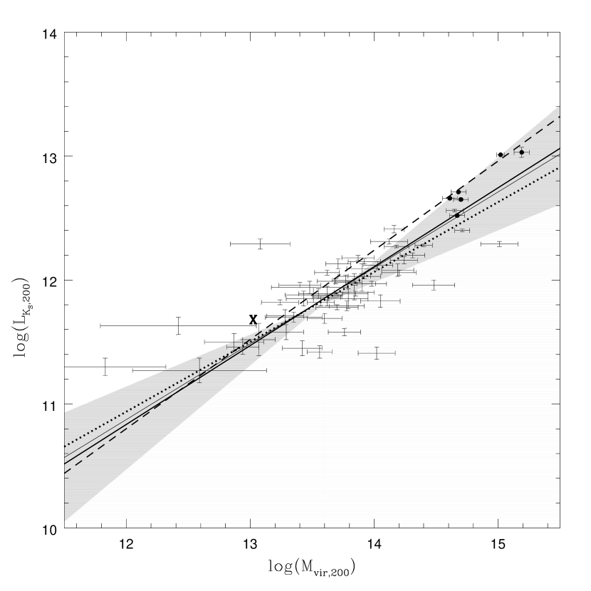
Figure 8: log($L_{K_{s},200}$) vs log($M_{vir,200}$) for the “expanded” sample of 55 groups and the 6 clusters of Rines et al. (2003) and Tustin et al. (2001) (black dots). The lines represent the relations for the “core” sample (dotted line), for the “expanded” sample (solid line), and for the sample including both the “expanded” sample and the 6 clusters of Rines et al. (2003) and Tustin et al. (2001) (thick solid line). The dashed line is L04 relation. The shaded area indicates the region between the two extreme estimators of the relation for the “core” sample. The letter “X” marks the luminosity and X–ray mass of NRGb045.

Figure 8 shows $M_{vir,200}$ and $L_{K_{s},200}$ for the total sample of 55 groups. In this case the BCES regression analysis leads to

$${\rm log}(L_{K_{s},200})=(0.56\pm 0.06)\,{\rm log}(M_{vir,200})+(4.17\pm 0.87).$$ (4)

Figure 8 shows the regression line for the total sample (dotted line) together with L04 regression line for $L_{K_{s},200}$ vs $M_{200}$ (dashed line). Clearly the behavior of $L_{K_{s},200}$ vs $M_{vir,200}$ for the extended sample agrees well with the result obtained for the core sample (thin solid line), again according to the Welch test. In Figure 8 we shade the area between the two extreme estimates of the regression line for our core sample (Akritas & Bershady 1996). All the regression lines of our various samples fall within the shaded area. The L04 best fit relation lies very close to (or within) the borders of this shaded area.

Our results extend the L04 relation to the low mass range $M_{200}<2\times 10^{13}$. Because there are so few systems within this mass range, we reconsider the special case of the system NRGb045, dropped from our virial theorem analysis because it has fewer than 5 members within $R_{200}$. NRGb045 is the only system in our sample which has an X–ray temperature unavailable to (and not considered by) L04. For this system Mahdavi et al. (2004) use a previously unpublished Chandra observations to compute the X–ray temperature T_X = 0.61$\pm$0.04 keV. To obtain a mass, we use the relation of Finoguenov et al. (2001) between T_X and $M_{500}$ scaled from $M_{500}$ to $M_{200}$ for a NFW profile with concentration $c=5$. We obtain log($M_{200}$) = 13.05. Finally we use all available members within 1.5 $h^{-1}$ Mpc down to $K_{s,lim}$ = 12.61 to derive a total luminosity log ($L_{K_{s},tot}$) = 11.69. We mark the position of NRGb045 with the symbol X in Figure 8. Clearly the low mass system NRGb045 provides further support for the equation (4).

The studies of L03 and L04 indicate that the same relation between $L_{K_{s},200}$ vs $M_{200}$ continues to be valid for masses exceeding those we sample. The details of their analysis differ from ours. For consistency across the entire range of system masses, we analyze recent cluster data from Rines et al. (2003) and Tustin et al. (2001) using the same approach we apply to the sample of poorer systems. This approach avoids systematic offsets which might result from different approaches to mass and/or luminosity estimation. Table 2 summarizes the observations and derived quantities for the 5 clusters surveyed by Rines et al. (2003) and for the cluster surveyed by Tustin et al. (2001). Figure 8 shows the Rines et al. (2003) and Tustin et al. (2001) clusters as black circles. Their position in the diagram agrees with the relation defined by the poorer systems. Including these clusters in the analysis makes a negligible change in the regression; the logarithmic slope is now

$${\rm log}(L_{K_{s},200})=(0.64\pm 0.06)\,{\rm log}(M_{vir,200})+(3.19\pm 0.79).$$ (5)

We represent this relation with a thick solid line in Figure 8.

Figure 9 shows the mass-to-light ratio, $M_{vir,200}/L_{K_{s},200}$, as a function of $M_{vir,200}$ for the expanded sample in Figure 8 including the Rines et al. (2003) and Tustin et al. (2001) clusters. We find

$${\rm log}(M_{vir,200}/L_{K_{s},200})=(0.56\pm 0.05)\,{\rm log}(M_{vir,200})-(5.98\pm 0.88).$$ (6)

As discovered by L03, $M_{vir,200}/L_{K_{s},200}$ increases for more massive, higher velocity dispersion systems.

Mass-to-light ratios of galaxies in the NIR vary by no more than a factor of 2 over a large range of star formation histories (e.g. Madau et al 1998; Bell & de Jong 2001; Bell 2003). On the theoretical side, a decrease of the differences in mass-to-light ratio toward NIR wavelengths with variations in stellar population is predicted by Bruzual & Charlot (2003). The observed/expected range of variation in $M_{vir,200}/L_{K_{s},200}$ for individual galaxies is clearly not enough to produce the observed trend of $M_{vir,200}/L_{K_{s},200}$ vs $M_{vir,200}$ for groups.

Uncertainty in the dynamical state of groups, and hence in the validity of the virial mass estimator, may contribute to the scatter in Figure 9. The uncertainty in the “true” mass resulting from a reasonable departure from the assumed dynamical state of groups is, on average, $\sim$30% – 40% (e.g. Giuricin et al. 1988; Diaferio et al. 1999). This uncertainty is unlikely to alter our results significantly. A change in mass by a factor of 1.3 without a corresponding change in luminosity would move any low mass group only slightly off the M/L relation. It is therefore impossible to explain the two order of magnitude variation of $M_{vir,200}/L_{K_{s},200}$ we observe over the whole $M_{vir,200}$ range as a result of evolutionary effects on the mass estimates.

Interlopers, possibly included as group members may also contribute to the scatter, particularly at the low mass end. However, the uncertainties in the luminosity that could be caused by interlopers are much smaller than the corresponding uncertainties produced in the mass (see for example the error bars in figure 8).

There are potential systematic variations in galaxy properties with the velocity dispersion of the system which might contribute to this relation. We assume a fixed form for the galaxy LF; it is possible that there are systematic variations particularly at the faint end. If, contrary to our assumption, the faint end is steeper for more massive systems, the $M_{vir,200}/L_{K_{s},200}$ would be reduced relative to less massive systems. There is some observational evidence for a larger dwarf-to-giant ratio, or equivalently a steeper faint-end slope in richer systems (Zabludoff & Mulchaey 2000). This effect however, cannot be solely responsible for the variation of the mass-to-light ratio we observe. We find an increase by a factor fifty over a mass interval of three orders of magnitudes. To explain the $M_{vir,200}/L_{K_{s},200}$ dependence within a mass range of only one order of magnitude, $\Delta log(M_{vir,200})$ = 1, the LF would have to steepen up to $\alpha\simeq-2.15$ well outside the observed range.

Variation in the galaxy population as a function of the velocity dispersion might also contribute to the dependence of $M_{vir,200}/L_{K_{s},200}$ on $M_{vir,200}$. Biviano et al. (1997) and Koranyi & Geller (2002) show that the fraction of emission-line galaxies increases as the velocity dispersion decreases. The color differences between emission- and absorption-line galaxies are, however, much smaller at infrared than at optical wavelengths. We showed in Section 3.1 that in some galaxies dust emission makes a significant contribution to the $K_{s}$–band luminosity, however these galaxies are remarkably rare within groups. Population effects are thus unlikely to make a significant contribution to the trend discovered by L03 and L04 and supported here.

Finally the contributions of the extended halo of the brightest cluster member and/or intracluster light to the total luminosity are not included in the 2MASS luminosity. The presence of intracluster red giant branch stars (Durrell et al. 2002), planetary nebulae (Ciardullo et al. 1998; Feldmeier er al. 1998; Durrell et al. 2002; Feldmeier et al. 2003). globular clusters (West et al. 1995; Jordán et al. 2003), diffuse light (e.g. Zwicky 1952; Melnick et al. 1977; Uson et al. 1991; Bernstein et al. 1995; Gregg & West 1998; Gonzalez et al. 2000), and supernovae (Gal-Yam et al. 2003) not associated with individual cluster members all suggest that stripped material contributes to intracluster light (Moore et al. 1999; Gnedin 2003). In rich clusters like those in the Rines et al. (2003) sample, various estimates indicate that intracluster light might constitute 5-50% of the light in the virial regions.

Two recent studies explore contribution of diffuse optical emission to the total luminosity of groups of galaxies. White et al. (2003) examine Hickson compact Group 90 and argue that 38%-48% of the total group light belongs to a diffuse component identified with tidal debris. Castro-Rodriguez et al. (2003) carried out a narrow band survey of the Leo I group to limit the number density of planetary nebulae in the group. They find none and set a stringent upper limit of 1.6% on the contribution of diffuse light to the total luminosity core of the group. As in rich clusters, the limits on the fractional contribution of diffuse light to the group luminosity have a similar and wide range from 1.6%-48%.

Recent simulations (Murante et al. 2004) indicate that for systems with masses exceeding 10¹⁴M_⊙, the fraction of stars in diffused light increases with cluster mass. They suggest that at least $\sim$10% of the stars in a cluster may be contributors to the intracluster light.

We conclude that the population effects on the relation in Figure 9 are small but that intracluster light could complicate the interpretation of the relation. Two plausible physical interpretations of this result are: (1) galaxy formation is less efficient in more massive systems and/or (2) galaxies are destroyed in collisions and tidal interactions in the more massive systems. In the second case, the disrupted material might appear as intracluster light which we do not detect. There are currently no data available which constrain the fraction of diffuse light as a function of the mass or velocity dispersion of the parent system.

5 Comparison with Previous Results

There are four previous analyses of masses and 2MASS luminosities of samples of systems of galaxies: Kochanek et al. (2003), L03, Rines et al. (2004) and L04. L03, L04, and Rines et al. (2004) all find a significant increase of $M_{200}/L_{K_{s},200}$ with the mass of the system. Kochanek et al. (2003) find no increase and perhaps a small decrease.

In comparing our results with L03 and L04, we focus our discussion on L04; their large sample of 93 clusters supersedes L03. Furthermore L04 and L03 give similar results. The L04 sample and ours probe overlapping but not coincident regions in the mass – luminosity plane. In particular our sample contains more low mass systems and fewer high mass systems than L04. The lowest quartile of the distribution of masses of L04 systems, $M_{Q25}=13\times 10^{13}$, is larger than our highest quartile, $M_{Q75}=11\times 10^{13}$. The lowest masses of our sample (about $10^{12}$) are more than one order of magnitude below L04 lowest masses ($10^{13}$). We expect this difference between the mass distributions of the two samples because L04 systems are X–ray selected. Even our X–ray emitting systems are not X–ray selected.

We select our initial “core” sample from a redshift survey and subsequently confirm the physical robustness of each system by X–ray detection; L04 select a sample of X–ray clusters. L04 estimate the total luminosity from de-projected and background corrected counts of galaxies at the position of X–ray emission peaks of the Abell clusters in their sample. They derive masses from X–ray temperatures whereas we use magnitudes and velocities of individual member galaxies selected in redshift space to derive a dynamical mass.

L04 fit log($L_{K_{s},200}$) vs log($M_{200}$) and obtain $d$ log($L_{K_{s},200}$)/ $d$ log($M_{200}$) = (0.72 +/- 0.04). We plot this relation in Figure 8 (dashed line). Clearly the L04 relation is indistinguishable from our regression lines; a Welch test verifies the visual impression. Given the completely different methods used to estimate masses and luminosities, Figure 8 demonstrates the robustness of the different estimates and of the physical result.

In the intermediate mass range spanned mostly by our “core” sample, there are two systems in common with L04. In the entire sample there are 9 objects in common (marked “l” in Table 1). L04 and our mass estimates differ for these objects: for 4 out of nine objects we find a lower mass and for the remaining objects we obtain a higher mass. The differences are typically a factor of 2 and the median mass ratio is 1.85. The system luminosities are in good agreement: the median ratio between L04 and our luminosities is 1.03 and the fractional differences never exceed 10%. In computing this ratio we make a geometric correction that decreases the luminosities in Table 1 by 20%: Table 1 lists luminosities projected in cylinders with a radius $R_{200}$ whereas L04 compute luminosities within a sphere. We also take the different faint magnitude cut-off of L04 into account (another 10% decrement of the luminosities in Table 1). The median differences between the mass and luminosity estimates yield a median mass-to-light ratio larger than L04 by about 50% for our overlapping systems. This difference corresponds to the median uncertainty on our individual mass-to-light ratios. The bias in the mass (without a corresponding bias in the luminosity) roughly preserves the logarithmic relation between mass-to-light ratio and mass we observe.

Because of the small number of overlapping systems, it is difficult to identify the reason for the differences between the mass estimates. Interlopers in our systems could artificially increase the velocity dispersion. Another possibility is that X–ray masses may systematically underestimate the mass of the system (Finoguenov et al. 2001; Girardi et al. 1998). Simulations by Rasia et al. (2003) also suggest the presence of a 30% - 50% bias in the direction we find for masses derived from $\beta$-models. Taking these potential biases into account could significantly reduce the observed differences between our masses and those of L04.

The agreement of our luminosity estimates with those of L04 means that the presence of a population of dusty objects (see Section 3.1) does not invalidate the statistical background subtraction of L04. Statistical background subtraction works here because these intrinsically luminous objects (with ($H-K_{s}$) $\gtrsim$ 0.35), are rarely, if ever, members of the nearby systems in our sample or in the sample of L04.

Our masses of the 5 systems in common with Rines et al. (2003) are larger by a median factor 1.5, systematically exceeding the masses obtained from caustics. By using the same analysis procedure for these clusters as for the core sample, we include galaxies in the member list that lie at high barycentric velocity and at relatively large radii; these galaxies are outside the caustics. The number of these galaxies is small, but their effect is rather large. We also expect our masses to be larger than those of Rines et al. (2003) because we do not correct for the surface term in the virial theorem (Carlberg et al. 1996; Girardi et al. 1998). There is no difference between our luminosity computations and those of Rines et al. (2003).

L04 find that the exclusion of the brightest member galaxy from each cluster leads to a steeper logarithmic slope of the $L_{K_{s},200}$ vs $M_{200}$ relation. As noted in Section 3.2, the narrow infrared color range of the brightest member galaxies of our sample (Section 3.1) gives some physical justification for this approach. We exclude the brightest galaxy from each group before the fit and find the steeper $d$ log($L_{K_{s},200}$) / $d$ log($M_{vir,200}$ ) = 0.74 +/- 0.06, consistent with the trend detected by L04.

L04 also plot log($M_{200}/L_{K_{s},200}$) vs log($M_{200}$) and fit it with a logarithmic slope $\simeq$ 0.3. Our slope, 0.56$\pm$0.05 is significantly steeper (figure 9). It is also steeper than expected on the basis of our $M_{vir,200}/L_{K_{s},200}$ vs $L_{K_{s},200}$ relation. One reason for this apparent inconsistency is the weighting of errors in the particular estimator of the regression line we use; the fractional errors in the mass are much larger than the fractional errors in the luminosity biasing the slope toward steeper values. Furthermore our error bars do not account for systematic uncertainties and thus the uncertainty in the slope is thus probably larger than implied by our estimated internal errors. The shaded area in Figure 8 shows that different estimators (Akritas & Bershady, 1996) of the slopes of $M_{vir,200}/L_{K_{s},200}$ vs $L_{K_{s},200}$ for the expanded sample have a large spread of (0.54, 0.74). This range of slopes yields a range of slopes for log($M_{200}/L_{K_{s},200}$) vs log($M_{200}$) which overlaps the L04 result.

Like L03, L04, and Rines et al. (2004), our results differ from those of Kochanek et al. (2003). L03 briefly comment that, in principle, their sample and the one built by Kochanek et al. (2003) should yield similar results but that the L04 estimates of the physical properties of individual systems is more robust that the corresponding estimates by Kochanek et al. (2003). Our selection of systems is more similar to the procedure followed by L03 and L04 than to the statistical approach based on structure formation simulations taken by Kochanek et al. (2003). The independent analyses of 55 systems in our sample, 93 systems in the L04 sample, and the 9 CAIRNS clusters (Rines et al. 2004) show that the increase of the NIR mass-to-light ratio with mass appears to be a robust property of systems of galaxies with masses ranging from 7$\times$10¹¹ to 1.5$\times$10¹⁵.

6 Conclusion

We use a sample of 55 groups and 6 clusters of galaxies ranging in mass from 7$\times$10¹¹ to 1.5 $\times$10¹⁵ to examine the correlation of the $K_{s}$–band luminosity with mass discovered by L03 and further investigated by L04 and Rines et al. (2004). We use complete redshift surveys of the 55 groups to explore the IR photometric properties of groups members including their IR color distribution and LF.

Although we find no significant difference between the $K_{s}$–band GLF and the general field determination by Kochanek et al. (2001), we do find a difference between the color distribution of luminous group members and their counterparts (generally background) in the field. There is a significant population of luminous galaxies with (($H-K_{s}$) $\gtrsim$ 0.35) which are rarely, if ever, members of the groups in our sample. The most luminous galaxies which populate the groups have a very narrow range of IR color.

Although we select and analyze our group sample with approaches completely different from those taken by L03 and L04, we find nearly the same dependence of $L_{K_{s},200}$ on $M_{200}$. The mass-to-light ratio of groups increases with the mass of the system. Out of the 55 groups plus 6 clusters we analyze, only 9 systems overlap with the analyses of L04.

We conclude, as have previous investigators of this issue, that galaxy formation is suppressed or galaxy disruption is enhanced in more massive systems. If disruption is the dominant process which accounts for the dependence of mass-to-light ratio on mass, more massive systems should harbor relatively more diffuse light. Recent simulations give some support to this proposal (Murante et al. 2004).

Neither our analysis nor that of L03 and L04 takes intracluster light into account. There are no data which set interesting limits on intra-system light as a function of system mass. These challenging observations would be an important contribution to the understanding of galaxy formation and evolution in galaxy systems.

Table 1: Basic data for 61 groups in the sample.

Group ID	$\alpha$ (J2000)	$\delta$ (J2000)	log10(Mvir,200/$h^{-1}$M${}_{\odot})$	log10(L${}_{K_{s},200}$/$h^{-2}$L${}_{K_{s},\odot})$	$r_{\mathrm{search}}$	Comments	Source
	(h m s)	(${}^{\mathrm{o}}\ {}^{\prime}\ {}^{\prime\prime}$)			($h^{-1}$ Mpc)
(1)	(2)	(3)	(4)	(5)	(6)	(7)	(8)
SRGb062	00 18 22.5	+30 04 00	13.84$\pm$ 0.13	12.03$\pm$ 0.02	1.50	X	M99
SRGb063	00 21 11.1	+22 18 56	13.62$\pm$ 0.10	12.06$\pm$ 0.02	1.50	X	MG04
SRGb102	01 25 55.8	+01 49 27	13.90$\pm$ 0.11	11.97$\pm$ 0.06	1.50	X	MG04
N664	01 44 02.7	+04 19 02	-	-	0.68	b	ZM88
SRGb119	01 56 13.8	+05 35 12	13.79$\pm$ 0.16	11.85$\pm$ 0.08	1.50	X	M99
SRGb145	02 32 28.6	+00 56 11	13.70$\pm$ 0.17	11.78$\pm$ 0.02	1.50	-	MG04
SRGb149	02 38 43.8	+02 01 11	13.90$\pm$ 0.12	12.09$\pm$ 0.04	1.50	-	MG04
SRGb155	02 50 19.2	+00 45 11	14.48$\pm$ 0.17	11.96$\pm$ 0.04	1.50	X	MG04
AWM7	02 54 27.5	+41 34 44	14.71$\pm$ 0.06	12.40$\pm$ 0.01	1.50	l, X	KG02
SRGb158	02 55 09.9	+09 16 43	13.55$\pm$ 0.16	11.89$\pm$ 0.04	1.50	X	MG04
N2563	08 20 24.4	+21 05 46	13.57$\pm$ 0.11	11.82$\pm$ 0.03	0.62	l, X	ZM98
NRGb004	08 38 07.3	+24 58 02	13.40$\pm$ 0.17	11.96$\pm$ 0.02	1.50	X	M99
NRGb007	08 50 29.9	+36 29 13	-	-	1.50	b	M99
NRGb025	09 13 37.3	+29 59 58	14.05$\pm$ 0.16	11.83$\pm$ 0.05	1.50	X	M99
NRGs027	09 16 20.8	+17 36 32	13.92$\pm$ 0.13	12.15$\pm$ 0.02	1.50	X	MG04
AWM1	09 16 49.9	+20 11 54	14.31$\pm$ 0.10	12.20$\pm$ 0.02	1.38	-	KG02
NRGb032	09 19 46.9	+33 45 00	14.03$\pm$ 0.12	12.12$\pm$ 0.03	1.50	l, X	M99
MKW1s	09 20 02.1	+01 02 18	-	-	0.47	b	KG02
NRGb043	09 28 16.2	+29 58 08	13.29$\pm$ 0.14	11.58$\pm$ 0.06	1.50	-	M99
NRGB045	09 33 25.6	+34 02 52	-	-	1.50	b, X	M99
NRGb057	09 42 23.2	+36 06 37	12.59$\pm$ 0.54	11.27$\pm$ 0.10	1.50	X	M99
SS2b144	09 49 59.9	– 05 02 48	12.87$\pm$ 0.24	11.50$\pm$ 0.07	1.50	-	MG04
H42	10 00 13.1	– 19 38 24	13.07$\pm$ 0.13	11.52$\pm$ 0.13	0.49	X	ZM98
MKW1	10 00 30.3	– 02 58 10	13.76$\pm$ 0.13	11.58$\pm$ 0.03	0.94	X	KG02
NRGs076	10 06 52.4	+14 27 31	15.01$\pm$ 0.15	12.29$\pm$ 0.02	1.50	X	MG04
NRGb078	10 14 01.8	+38 56 09	13.77$\pm$ 0.11	12.00$\pm$ 0.04	1.50	-	MG04
NRGs110	10 59 09.9	+10 00 31	14.12$\pm$ 0.15	12.31$\pm$ 0.02	1.50	X	MG04
NRGs117	11 10 42.9	+28 41 38	14.65$\pm$ 0.07	12.56$\pm$ 0.01	1.50	l, X	M99
NRGs127	11 21 34.2	+34 15 31	13.08$\pm$ 0.24	12.29$\pm$ 0.04	1.50	-	M99
SS2b164	11 23 15.8	– 07 51 30	13.78$\pm$ 0.14	11.79$\pm$ 0.04	1.50	X	MG04
MKW10	11 42 23.7	+10 15 51	12.42$\pm$ 0.63	11.63$\pm$ 0.07	0.70	X	KG02
NRGs156	11 45 33.3	+33 14 46	13.48$\pm$ 0.31	11.94$\pm$ 0.05	1.50	X	MG04
MKW4	12 04 27.2	+01 53 43	14.24$\pm$ 0.11	12.16$\pm$ 0.03	1.26	l, X	KG02
MKW4s	12 06 38.9	+28 10 26	14.19$\pm$ 0.13	12.08$\pm$ 0.05	1.50	l, X	KG02
NRGb181	12 07 35.5	+31 26 32	-	-	1.50	b	M99
NRGb184	12 08 55.9	+25 17 33	13.79$\pm$ 0.11	11.98$\pm$ 0.01	1.50	X	MG04
AWM2	12 15 37.6	+23 58 55	13.60$\pm$ 0.14	11.69$\pm$ 0.04	0.99	-	KG02
N4325	12 23 18.2	+10 37 19	13.42$\pm$ 0.16	11.45$\pm$ 0.06	0.95	X	ZM98
H62	12 52 57.9	– 09 09 26	13.85$\pm$ 0.10	11.89$\pm$ 0.02	0.56	l, X	ZM98
NRGs241	13 20 27.3	+33 12 01	14.18$\pm$ 0.10	12.27$\pm$ 0.01	1.50	X	MG04
NRGb244	13 23 57.9	+14 02 37	13.43$\pm$ 0.14	11.85$\pm$ 0.06	1.50	X	M99
NRGb247	13 29 25.7	+11 45 21	13.92$\pm$ 0.13	12.03$\pm$ 0.02	1.50	X	M99
NRGb251	13 34 25.3	+34 41 25	13.50$\pm$ 0.24	11.88$\pm$ 0.06	1.50	a, X	M99
SS2b239	13 48 51.5	– 07 26 59	13.62$\pm$ 0.12	11.87$\pm$ 0.08	1.50	X	MG04
MKW5	14 00 37.4	– 02 51 29	13.28$\pm$ 0.15	11.71$\pm$ 0.05	0.78	-	KG02
MKW12	14 02 48.0	+09 19 40	13.24$\pm$ 0.15	11.82$\pm$ 0.02	1.19	-	KG02
AWM3	14 28 12.7	+25 50 39	13.56$\pm$ 0.10	11.42$\pm$ 0.05	1.34	X	KG02
NRGb302	14 28 29.8	+11 29 20	13.62$\pm$ 0.11	11.86$\pm$ 0.02	1.50	X	MG04
MKW8	14 40 42.9	+03 27 53	13.87$\pm$ 0.13	12.18$\pm$ 0.02	0.81	l	KG02
NRGs317	14 47 05.3	+13 39 46	13.70$\pm$ 0.13	11.99$\pm$ 0.02	1.50	X	M99
N5846	15 05 47.0	+01 34 25	-	-	0.24	c, X	ZM98
AWM4	16 04 56.8	+23 55 58	13.84$\pm$ 0.16	11.90$\pm$ 0.06	0.56	l, X	KG02
NRGs385	16 17 43.9	+34 58 00	14.39$\pm$ 0.08	12.28$\pm$ 0.01	1.50	X	MG04
AWM5	16 57 58.0	+27 51 16	14.16$\pm$ 0.08	12.41$\pm$ 0.03	0.73	X	KG02
H90	22 02 31.4	– 32 04 58	12.94$\pm$ 0.13	11.46$\pm$ 0.06	0.33	X	ZM98
SRGb009	22 14 46.0	+13 50 30	13.97$\pm$ 0.12	11.97$\pm$ 0.02	1.50	X	M99
SRGb013	22 50 21.1	+11 34 47	14.21$\pm$ 0.13	12.06$\pm$ 0.02	1.50	X	MG04
SRGb016	22 58 45.9	+26 00 05	13.71$\pm$ 0.10	12.13$\pm$ 0.04	1.50	X	M99
N7582	23 18 54.5	– 42 18 28	11.83$\pm$ 0.49	11.30$\pm$ 0.07	0.21	-	ZM98
SRGb037	23 29 57.6	+03 40 56	14.02$\pm$ 0.15	11.41$\pm$ 0.05	1.50	-	MG04
SS2b312	23 47 51.6	– 02 20 16	13.36$\pm$ 0.22	11.70$\pm$ 0.04	1.50	X	MG04

Note. — Columns: (1) Name; (2) Right Ascension; (3) Declination; (4) Virial mass within $R_{200}$; (5) $K_{s}$-band luminosity within $R_{200}$; (6) Search radius; (7) Comments; (8) Reference for data source.

Table 2: Basic data for six Abell clusters.

Group ID	$\alpha$ (J2000)	$\delta$ (J2000)	log10(Mvir,200/$h^{-1}$M${}_{\odot})$	log10(L${}_{K_{s},200}$/$h^{-2}$L${}_{K_{s},\odot})$	$r_{\mathrm{search}}$	Source
	(h m s)	(${}^{\mathrm{o}}\ {}^{\prime}\ {}^{\prime\prime}$)			($h^{-1}$ Mpc)
(1)	(2)	(3)	(4)	(5)	(6)	(7)
A496	04 33 35.2	– 13 14 45	14.61$\pm$ 0.06	12.66$\pm$ 0.01	1.50	R03
A539	05 16 32.1	+06 26 31	14.67$\pm$ 0.06	12.52$\pm$ 0.01	1.50	R03
A1367	11 44 36.2	+19 46 19	14.70$\pm$ 0.06	12.65$\pm$ 0.01	1.50	R03
A1644	12 57 11.6	– 17 24 34	15.19$\pm$ 0.06	13.03$\pm$ 0.04	1.50	T01
A1656 (Coma)	12 59 31.9	+27 54 10	15.02$\pm$ 0.03	13.01$\pm$ 0.01	1.50	R03
A2199	16 28 39.5	+39 33 00	14.68$\pm$ 0.06	12.71$\pm$ 0.01	1.50	R03

Note. — Columns: (1) Name; (2) Right Ascension; (3) Declination; (4) Virial mass within $R_{200}$; (5) $K_{s}$-band luminosity within $R_{200}$; (6) Search radius; (7) Reference for data source.

Figure 1: ($J-K_{s}$) color distribution of members (solid line) and non-members (dot- dashed line). The four panels (I to IV) are for galaxies of decreasing luminosity: from galaxies brighter than the first quartile of the absolute magnitude distribution (class I) to galaxies fainter than the third quartile (class IV).

Figure 2: ($J-K_{s}$) color vs absolute magnitude of members (filled circles) and non-members (empty circles). Galaxies are those brighter than the first quartile of the absolute magnitude distribution (class I). The sizes of the circles are proportional to the redshifts (larger circles represent more distant objects).

Figure 3: Color - color diagram for the brightest galaxies (class I). Dots represent members, crosses are non-members. The arrow represents the reddening vector.

Figure 4: Redshift distribution of members (solid line) and non-members (dot- dashed line). The four panels (I to IV) are for galaxies of decreasing luminosity: from galaxies brighter than the first quartile of the absolute magnitude distribution (class I) to galaxies fainter than the third quartile (class IV).

Figure 5: Total “observed” histogram (dotted line) of absolute magnitudes of members, $H_{o}(\Delta_{M})$, and total “expected” histogram $H_{e}(\Delta_{M})$ (solid line) computed for a Schecter LF with the best fit parameters ($M_{K_{s}}^{*},\alpha)_{bf}$ = (-23.55, -0.84). These values are marked with a dot in the inset. The inset also shows 1-$\sigma$ and 2-$\sigma$ c.l. contours.

Figure 6: Best fit parameters (dots) and 1-$\sigma$, 2-$\sigma$ c.l. contours obtained for a single simulated system with ($M_{K_{s}}^{*},\alpha)$ = (-23.4, -1.1) within a given absolute magnitude limit, $M_{K_{s},lim,sim}$. Panels A to D are for $M_{K_{s},lim,sim}$ = -22.0, -21, -19., and -17.0 respectively.

Figure 7: log($L_{K_{s},200}$) vs log($M_{vir,200}$) for the “core” sample of 36 groups from Mahdavi et al. (1999) and Mahdavi & Geller (2004). The line represents the relation of equation 3.

Figure 9: log($M_{vir,200}/L_{K_{s},200}$) vs log($M_{vir,200}$) for the “expanded” sample of 55 groups and the 6 clusters of Rines et al. (2003) and Tustin et al. (2001) (black dots). The line represents the relation of equation 6.

References

- (1) Akritas, M.G., & Bershady, M.A. 1996, ApJ, 470, 706
- (2) Andreon, S. 2004, å, 416, 865
- (3) Bahcall, N.A., Cen, R., Dav , R., Ostriker, J.P., & Yu, Q. 2000, ApJ, 541, 1
- (4) Bahcall, N.A., & Comerford, J.M. 2002, ApJ, 565, L5
- (5) Balogh, M.L., Christlein, D., Zabludoff, A.I., & Zaritsky, D. 2001, ApJ, 557, 117
- (6) Balogh, M.L., Eke, V., Miller, C., et al. 2004, MNRAS, 348, 1355
- (7) Bell, E.F., & de Jong, R.S. 2001, ApJ, 550, 212
- (8) Bell, E.F., McIntosh, D.H., Katz, N., & Weinberg, M.D. 2003 ApJS, 149, 289
- (9) Bernstein, G.M., Nichol, R.C., Tyson, J.A., Ulmer, M.P., & Whittman, D. 1995, AJ, 110, 1507
- (10) Biviano, A., Katgert, P., Mazure, A., et al. 1997, A&A, 321, 84
- (11) Bruzual, G. & Charlot, S. 2003, MNRAS, 344, 1000
- (12) Carlberg, R.G., Yee, H.K.C., Ellingson, E., et al. 1996, ApJ, 462, 32
- (13) Carlberg, R.G., Yee, H.K.C., Ellingson, E., et al. 1997, ApJ, 485, L13
- (14) Carlberg, R.G., Yee, H.K.C., Morris, S.L., Lin, H., Hall, P.B., Patton, D.R., Sawicki, M. & Shepherd, C.W. 2001, ApJ, 552, 427
- (15) Castro-Rodriguez, N., Aguerri, J.A.L., Arnaboldi, M., et al. 2003, A&A, 405, 803
- (16) Cen, R. 1997, ApJ, 485, 39
- (17) Christlein, D., & Zabludoff, A.I. 2003, ApJ, 591, 764
- (18) Ciardullo, R., Jacoby, G.H., Feldmeier, J.J., & Bartlett, R.E. 1998, ApJ, 492, 62
- (19) Cole, S., Norberg, P., Baugh, C.M., et al. 2001, MNRAS, 326, 255
- (20) Colless, M. 1989, MNRAS, 237, 799
- (21) De Propris, R., Colless, M., Driver, S.P., et al. 2003, MNRAS, 342, 725
- (22) Diaferio, A., Kauffmann, G., Colberg, J.M., & White, S.D.M. 1999, MNRAS, 307, 537
- (23) Durrell, P.R., Ciardullo, R., Feldmeier, J.J., Jacoby, G.H., & Sigurdsson, S. 2002, ApJ, 570, 119
- (24) Ellis, S.C., & Jones, L.R. 2004, MNRAS, 348, 165
- (25) Faber, S.M., & Gallagher, J.S. 1979, ARA&A, 17, 135
- (26) Feldmeier, J.J., Ciardullo, R., & Jacoby, G.H. 1998, ApJ, 503, 109
- (27) Feldmeier, J.J., Ciardullo, R., Jacoby, G.H., & Durrell, P.R. 2003, ApJS, 145, 65
- (28) Fioc, M., & Rocca-Volmerange, B. 1999, A&A, 351, 869
- (29) Finoguenov, A., Reiprich, T.H., & Böhringer, H. 2001, A&A, 368, 749
- (30) Flint, K., Metevier, A.J., Bolte, M., & Mendes de Oliveira, C. 2001, ApJS, 134, 53
- (31) Francis, P.J., Nelson, B.O., & Cutri, R.M. 2004, AJ, 127, 646
- (32) Gal-Yam, A., Maoz, D., Guhathakurta, P., & Filippenko, A.V. 2003, AJ, 125, 1087
- (33) Garilli, B., Maccagni, D., & Andreon, S. et al. 1999, A&A, 342, 408
- (34) Gavazzi, G., Pierini, D., & Boselli, A. 1996, A&A, 312, 397
- (35) Giovanardi, C., & Hunt, L.K. 1988, AJ, 95, 408
- (36) Girardi, M., Giuricin, G., Mardirossian, F., Mezzetti, M., & Boschin, W. 1998, ApJ, 505, 74
- (37) Girardi, M., Borgani, S., Giuricin, G., Mardirossian, F., & Mezzetti, M. 2000, ApJ, 530, 62
- (38) Girardi, M., Manzato, P., Mezzetti, M., Giuricin, G., & Limboz, F. 2002, ApJ, 569, 720
- (39) Giuricin, G., Gondolo, P., Mardirossian, F., Mezzetti, M., & Ramella, M. 1988, A&A, 199, 85
- (40) Gnedin, O.Y. 2003, ApJ, 589, 752
- (41) Gonzalez, A.H., Zabludoff, A.I., Zaritsky, D., & Dalcanton, J.J. 2000, ApJ, 536, 561
- (42) Goto, T., Okamura, S., McKay, T.A., et al. 2002, PASJ, 54, 515
- (43) Gott, J.R. III, & Turner, E.L. 1977, ApJ, 213, 309
- (44) Gregg, M.D., & West, M.J. 1998, Nature , 396, 549
- (45) Gregory, S.A, & Thompson, L.A. 1978, Nature, 274, 450
- (46) Guest, P.G. 1961, “Numerical methods of curve fitting”, pag. 107
- (47) Hunt, L.K., & Giovanardi, C. 1992, AJ, 104, 1018
- (48) Hunt, L.K., Giovanardi, C., & Helou, G. 2002, A&A, 394, 873
- (49) Huchra, J.P., & Geller, M.J. 1982, ApJ, 257, 423
- (50) James, P.A., & Seigar, M.S. 1999, A&A, 350, 791
- (51) Jarrett, T.H., Chester, T., Cutri, R., et al. 2000, AJ, 119, 2498
- (52) Jarrett, T.H., Chester, T., Cutri, R., Schneider, S.E., & Huchra, J.P. 2003, AJ, 125, 525
- (53) Jordán, A., West, M.J., Côté, P., & Marzke, R.O. 2003, AJ, 125, 1642
- (54) Kochanek, C.S., Pahre, M.A., Falco, E.E., et al. 2001, ApJ, 560, 566
- (55) Kochanek, C.S., White, M., Huchra, J., et al. 2003, ApJ, 585, 161
- (56) Koranyi, D.M., & Geller, M.J. 2002, AJ, 123, 100
- (57) Lilliefors, H.W. 1967, ASA Journal, June, 399-402
- (58) Lin, Y., Mohr, J.J., & Stanford, S.A. 2003, ApJ, 591, 749 (L03)
- (59) Lin, Y., Mohr, J.J., & Stanford, S.A. 2004, ApJ, preprint doi:10.1086/421714 (L04)
- (60) Lumsden, S.L., Collins, C.A., Nichol, R.C., Eke, V.R., & Guzzo, L. 1997, MNRAS, 290, 119L
- (61) Madau, P., Pozzetti, L., & Dickinson, M. 1998, ApJ, 498, 106
- (62) Mahdavi, A., Geller, M.J., Bohringer, H., Kurtz, M.J., & Ramella, M. 1999, AJ, 518, 69
- (63) Mahdavi, A., Böhringer, H., Geller, M.J. & Ramella, M. 2000, ApJ, 534, 114
- (64) Mahdavi, A., & Geller, M.J. 2004, ApJ, 607, 202
- (65) Mahdavi, A., et al. 2004, in preparation
- (66) Malumuth, E.M., & Kriss, G.A. 1986, ApJ, 308, 10
- (67) McLean, B.J., Greene, G.R., Lattanzi, M.G., & Pirenne, B. 2000, PASP, 216, 145
- (68) Melnick, J., Hoessel, J., & White, S.D.M. 1977, MNRAS, 180, 207
- (69) Mendes de Oliveria, C., & Hickson, P. 1991, ApJ, 380, 30
- (70) Moore, B., Lake, G., Quinn, T., & Stadel, J. 1999, MNRAS, 304, 465
- (71) Murante, G., Arnaboldi, M., Gerhard, O., Borgani, S., Cheng, L.M., Diaferio, A., Dolag, K., Moscardini, L., Tormen, G., Tornatore, L., & Tozzi, P. 2004, ApJ607, 83L
- (72) Navarro, J.F., Frenk, C.S., & White, S.D.M. 1997, ApJ, 490, 493
- (73) Paolillo, M., Andreon, S., Longo, G., et al. 2001, A&A, 367, 59
- (74) Peletier, R.F., Valentijn, E.A., & Jameson, R.F. 1990, A&A, 233, 62
- (75) Poggianti, B.M. 1997, A&AS, 122, 399
- (76) Ramella, M., Pisani, A., & Geller, M.J. 1997, AJ, 113, 483
- (77) Ramella, M., Zamorani, G., Zucca, E., et al. 1999, å, 342, 1
- (78) Rasia, E., Tormen, G., & Moscardini, L. 2003, MNRAS, submitted (astro-ph 0309405)
- (79) Rauzy, S., Adami, C., & Mazure, A. 1998, A&A, 337, 31
- (80) Rines, K., Geller, M.J., Kurtz, M.J., & Diaferio, A. 2003, AJ, 126, 2152
- (81) Rines, K., Geller, M.J., Diaferio, A., Kurtz, M.J., & Jarrett, T.H. 2004, AJ, submitted (astro-ph/0402242)
- (82) Schechter, P. 1976, ApJ, 203, 297
- (83) Terndrup, D.M., Davies, R.L., Frogel, J.A., Depoy, D.L., & Wells, L.A. 1994, ApJ, 432, 518
- (84) Tucker, D.L., Oemler, A. Jr., Hashimoto, Y., Shectman, S.A., Kirshner, R.P., Lin, H., Landy, S.D., Schechter, P.L., Allam, S.S. 2000, ApJS, 130, 237
- (85) Tustin, A.W., Geller, M.J., & Kenyon, S.J. 2001, A&A, 122, 1289
- (86) Uson, J.M., Boughn, S.P., & Kuhn, J.R. 1991, ApJ, 369, 46
- (87) Valotto, C.A., Nicotra, M.A., Muriel, H., & Lambas, D.G. 1997, ApJ, 479, 90
- (88) West, M.J., Côté, P., Jones, C., Forman, W., & Marzke, R.O. 1995, ApJ, 453, L77
- (89) White, P.M., Bothun, G.D., Guerrero, M.A., West, M.J., & Barkhouse, W.A. 2003, ApJ, 585, 739
- (90) Zabludoff, A.I., & Mulchaey, J.S. 1998, ApJ, 496, 39
- (91) Zabludoff, A.I., & Mulchaey, J.S. 2000, ApJ, 539, 136
- (92) Zibetti, S., Gavazzi, G.; Scodeggio, M., Franzetti, & P., Boselli, A. 2002, ApJ, 579, 261
- (93) Zwicky, F. 1952, PASP, 64, 242
- (94) Zwicky, F., Herzog, E., Wild, P., & Kowal, C., 1961-1968 Catalogue of Galaxies and of Clusters of Galaxies, Pasadena: California Institute of Technology