The Color-Magnitude Effect in Early-Type Cluster Galaxies

Abstract

We present the analysis of the color-magnitude relation (CMR) for a sample of 57 X-ray detected Abell clusters within the redshift interval $0.02\leq z\leq 0.18$. We use the $B-R$ vs $R$ color-magnitude plane to establish that the CMR is present in all our low-redshift clusters and can be parameterized by a single straight line. We find that the CMRs for this large cluster sample of different richness and cluster types are consistent with having universal properties. The k-corrected color of the individual CMRs in the sample at a fixed absolute magnitude have a small intrinsic dispersion of $\sim 0.05$ mag. The slope of the CMR is consistent with being the same for all clusters, with the variations entirely accountable by filter band shifting effects. We determine the mean of the dispersion of the 57 CMRs to be 0.074 mag, with a small rms scatter of 0.026 mag. However, a modest amount of the dispersion arises from photometric measurement errors and possible background cluster superpositions; and the derived mean dispersion is an upper limit. Models which explain the CMR in terms of metallicity and passive evolution can naturally reproduce the observed behavior of the CMR in this paper. The observed properties of the CMR are consistent with models in which the last episode of significant star formation in cluster early-type galaxies occurred significantly more than $\sim 3$ Gyr ago, and that the core set of early-type galaxies in clusters were formed more than 7 Gyr ago.

The universality of the CMR provides us with an important tool for cluster detection and redshift estimation. A very accurate photometric cluster redshift estimator can be devised based on the apparent color-shift of the CMR due to redshift. This calibrator has the additional advantage of being very efficient since only two bands are needed. An empirically calibrated redshift estimator based on the $B-R$ color of the CMR for clusters with $z<0.20$ produces an accuracy of $\Delta z\sim 0.010$. Background clusters, typically at $z\sim 0.25$ and previously unknown, are found in this survey in the color-magnitude diagrams as secondary CMRs to the red of the target cluster CMRs. We also find clear cases of apparent X-ray substructure which are due to these cluster superpositions. This suggests that X-ray observations of clusters are also subject to a significant amount of projection contaminations.

1. Introduction

Early-type galaxies are the dominant population in low-redshift galaxy clusters (e.g., Dressler, 1984; Kormendy & Djorgovski, 1989). When compared with other galaxy types, early-type galaxies can be labeled as a homogeneous class in terms of the dynamical structure, stellar populations, and the gas and dust content. The remarkable uniformity of the properties of early-type galaxies in clusters and the tightness of their fundamental plane and its projections suggest that these galaxies are coeval, had their last episode of strong star formation at high redshift ($z~{}\geq~{}2$), and have evolved passively since then (e.g., Bower, Lucey, & Ellis, 1992; Aragón-Salamanca et al., 1993; Pahre et al., 1996; van Dokkum et al., 1998; Stanford, Eisenhardt, & Dickinson, 1998; Gladders et al., 1998; López-Cruz et al., 2002; Blakeslee et al., 2003). As larger samples of early-type galaxies become available, the idea that giant spheroidal galaxies had their major starburst at high redshifts, regardless of the environment, becomes more popular (e.g., Peebles, 2002).

One of the properties of early-type galaxies that can be studied most straightforwardly is the color-magnitude relation (CMR). This effect was discovered by Baum (1959) who noted that field elliptical colors become redder as the galaxies become brighter. Baum’s study also revealed that the average colors of ellipticals are much redder than those of globular clusters, and concluded, contrary to Baade (1944), that elliptical galaxies were dominated by old Population I stars. To arrive at this conclusion, Baum generated a simple population synthesis model that was based on the, then novel, idea of progressive metal enrichment of a population by successive generations of stars (Fowler & Greenstein, 1956; Struve, 1956). Hence, elliptical galaxies may have experienced an extended period of very efficient star formation during the early stages of their formation. This idea is now accepted, but still debatable in terms of our inability to disentangle the effects of age and metallicity in present day ellipticals (e.g., Worthey et al., 1995; Ferreras, Charlot, & Silk, 1999).

A simple straight line fit can describe the CMR for elliptical galaxies in an interval of about 8 magnitudes in Virgo (e.g., Sandage, 1972) and Coma (e.g., Thompson & Gregory, 1993; López-Cruz, 1997; Secker, Harris, & Plummer, 1998). This effect is remarkable because it covers a range in luminosity of about $10^{3}$, suggesting that within this range galaxies have shared a similar evolutionary process. However, this is not the only way to get such an effect. For instance, the CMR can be reproduced by demanding younger galaxies to be more metal rich than older galaxies of similar luminosity (Ferreras, Charlot, & Silk, 1999). The potential of the CMR as a tool for cosmological studies was recognized by Sandage (1972) and was characterized for different galaxy environments (Visvanathan & Sandage, 1977; Sandage & Visvanathan, 1978a, b). The CMR’s application as a distance indicator has been suggested by Visvanathan & Sandage (1977). The dispersion in the CMR, which is very small, has been quantified for Virgo and Coma by Bower, Lucey, & Ellis (1992, hereafter BLE) and for high-redshift clusters (e.g., Ellis et al., 1997; van Dokkum et al., 1998; Stanford, Eisenhardt, & Dickinson, 1998; Gladders et al., 1998; Blakeslee et al., 2003). These studies have used the dispersion to constrain the epoch of galaxy formation and the way they have evolved.

The CMR was modeled as a metallicity effect by Arimoto & Yoshii (1987). The models of Arimoto & Yoshii incorporated the ideas of Larson (1974a, b) in which early-type galaxies are formed by dissipative monolithic collapse and the star formation regulated by supernova driven winds. As in Bower et al. (1998), we will call Larson’s model the classical model. More recently, Kodama (1997) and Kodama & Arimoto (1997, hereafter KA97) have revised the models of Arimoto & Yoshii (1987) and have included improved libraries for stellar evolution, incorporating the effects of the variation of metallicity with galaxy mass. Alternatively, the semi-analytical modeling of Kauffmann & Charlot (1998), which incorporate the hierarchical galaxy formation scenario, can also reproduce the CMR for early-type galaxies by imposing a very early epoch for the major mergers. Much effort has been devoted to improving the models and the observations; however, it is still difficult to decide whether early-type galaxies formed according to the hierarchical or the classical model (Bower et al., 1998, and references therein).

If cluster early-type galaxies were formed at high redshift, are coeval and evolving passively, then it should be expected that the CMR is universal at the current epoch. Universality should be defined in the present context as the validity for all clusters of the same rest-frame parameters: slope, intercept and dispersion. The works of Sandage & Visvanathan(Visvanathan & Sandage, 1977; Sandage & Visvanathan, 1978a, b) and BLE made a case for the universality of the CMR for early-type galaxies, albeit based on a few local clusters. There are other studies that appear to agree with these results (e.g., Butcher & Oemler, 1984; Dixon, Godwin, & Peach, 1989; Metcalfe et al., 1994; Garilli et al., 1996, and references therein). However, some apparent cluster-to-cluster variations of the CMR have also been reported, but the evidence is not compelling. For example, Aaronson, Persson, & Frogel (1981) reported that the $U-V$ and $V-K$ colors for galaxies in Coma were bluer than those for galaxies in Virgo; this result was not confirmed by BLE. Drastic changes in the CMR’s slope for galaxies within the same cluster have been reported (Metcalfe et al., 1994, and references therein). The model of galactic cannibalism proposed by Hausman & Ostriker (1978) hinted at an explanation for this phenomenon. However, most of the studies at different redshifts, even as high as $z\approx 0.5$ (Ellis et al., 1997) or higher (Stanford, Eisenhardt, & Dickinson, 1998; Gladders et al., 1998), have shown little indications of such an effect. The studies mentioned above utilized relatively small cluster samples and accurate photometry was limited mainly to the few nearest clusters. In this paper we show that the CMR in a 57-cluster sample at low redshifts, with different richness, cluster types and X-ray luminosities, are consistent with being universal.

This paper is the second of a series resulting from a large multicolor imaging survey of low-redshift Abell clusters. The paper is organized as follows. In §2 we present the sample selection criteria. In §3 we briefly describe the observations and photometric reduction procedures. Section 4 describes the CMR parameterization and the error estimate techniques; while §5 examines the dispersion of the CMR. We present a discussion of the results, in particular regarding the universality and the evolutionary models, in §6. In §7 we introduce some observational applications of the CMR based on the results of this study, including using the CMR as a redshift indicator and a cluster finding tool. Finally in §8 we summarize the conclusions. More details regarding sample selection, observations, image preprocessing, catalogs and finding charts can be found in López-Cruz (1997), Barkhouse (2003), and Barkhouse, López-Cruz, & Yee (2004a, in preparation, Paper I of this series). A detailed discussion of the luminosity function of cluster galaxies using this survey can be found in Paper III (Barkhouse, Yee, & López-Cruz 2004b, in preparation). Paper IV describes the characteristics of various color-selected cluster galaxies (Barkhouse, Yee, & López-Cruz 2004c, in preparation). Recent cosmological observations indicate that the best world model agrees with a flat $\Lambda$-dominated universe that is characterized by $\Omega_{\rm m}\simeq 0.3$, $\Omega_{\Lambda}\simeq 0.7$ and $H_{\circ}\simeq 70$ km s^-1 Mpc^-1 (e.g., Spergel et al., 2003). However, considering that the effects of dark energy and curvature are negligible at low redshifts ($z<0.2$) and in order to allow direct comparisons with previous studies; we, then, for convenience have set, unless otherwise indicated, $H_{\circ}=50h_{50}~{}\mbox{km}~{}\mbox{s}^{-1}~{}\mbox{Mpc}^{-1}$ and $q_{0}=0$ throughout this paper.

2. The Sample and Observations

The sample contains Abell clusters selected mainly from a compilation of bright X-ray clusters from Einstein’s IPC made by Jones & Forman (1999). The selection of clusters identified by independent techniques (i.e., optical and X-ray) reduces the probability of confusing real, gravitationally bound clusters, with apparent galaxy over-densities due to projection effects. The initial sample was defined under the following selection criteria: 1) the clusters should be at high galactic latitude, $|b|\geq 30\arcdeg$; 2) their redshifts should lie within the range $0.04\leq z\leq 0.20$; 3) the Abell richness class (ARC) should, preferably, be greater than 0; and 4) the declination $\delta\geq 20\arcdeg$. We attempt to follow these criteria strictly; however, some ARC=0 clusters were included due to observational constraints, such as the lack of suitable clusters at certain right ascensions during the observations. The ARC=0 clusters were not selected at random, but on the appearance of the X-ray emission and the Bautz-Morgan type that indicate a higher richness class. See Yee & López-Cruz (1999) for a discussion of the richness of the cluster sample.

This sample includes 47 clusters of galaxies observed in Kron-Cousins $B$, $R$, and $I$ at KPNO with the 0.9m telescope using the $2048\times 2048$ pixels T2KA CCD (López-Cruz, 1997; Yee & López-Cruz, 1999; López-Cruz, 2001, hereafter the LOCOS sample). In addition, two clusters imaged in $B$ and $R$ were included from Brown (1997) using the same instrumental setup and satisfying our selection criteria. We note that only the $B$ and $R$ data are considered in this paper. The field covered by this combination of a small telescope plus a 2K CCD is $23.2\arcmin\times 23.2\arcmin$ with a scale of $0.68\arcsec/\mbox{pixel}$, i.e., $\sim 1.5h_{50}^{-1}~{}\mbox{Mpc}$ at $z=0.04$ and $\sim 6h_{50}^{-1}\mbox{Mpc}$ at $z=0.2$.

A sub-sample of eight clusters from Barkhouse (2003) are included to complement our 49 cluster sample by covering the low redshift interval from $0.02\leq z\leq 0.04$. The data were obtained at KPNO with the 0.9m telescope using the 8k Mosaic camera ($8192\times 8192$ pixels). This telescope/detector combination yields a scale of $0.423\arcsec/\mbox{pixel}$, with a field-of-view of one square degree ($\sim 2h_{50}^{-1}~{}\mbox{Mpc}$ at $z=0.02$ and $\sim 4h_{50}^{-1}~{}\mbox{Mpc}$ at $z=0.04$). The clusters from this sample were selected using the previous criteria except that ARC=0 clusters were not preferentially excluded, although all clusters in the sample are detected in X-rays and have a prominent CMR.

The integration times for our 57 cluster sample varied from 250 to 9900 seconds, depending on the filter and the redshift of the cluster. The photometric calibrations were done using stars from Landolt (1992). Control fields are also an integral part of this survey. We observed in both $R$ and $B$ filters a total of 6 control fields chosen at random positions on the sky at least $5\arcdeg$ away from the clusters in the sample. These control fields were observed using the T2KA CCD and the Mosaic camera to a comparable depth and reduced in the same manner as the cluster data. All observations included in this study were carried out during 1992–93 and 1996–98.

Table 1 lists the sample with the cluster redshifts. Coma (A1656) was included in the LOCOS sample despite its low redshift ($z=0.0232$). The main reason for its inclusion is the vast amount of data for Coma available in the literature, which allows us to make direct comparisons of our results with others. (We note that only $R$ images of Coma were obtained with the Mosaic camera and hence are not considered here.)

3. Photometric Reductions

The preprocessing of the images was done using IRAF. The photometric reduction was carried out using the program PPP(Picture Processing Package, Yee, 1991), which includes algorithms for performing automatic object finding, star/galaxy classification and total magnitude determination. We also exploited a series of improvements to PPP described in Yee, Ellingson, & Carlberg (1996) which decrease the detection of false objects and allow star/galaxy classification in images with variable point-spread function (PSF). We describe the reduction procedures briefly below; full details are given in Paper I.

3.1. Photometry

The object list for each cluster is compiled from the R frames. The R frames are chosen because they are deeper than the images from the other filters. On average, about 3000 objects are detected in each LOCOS fields and about 25,000 objects in the mosaic fields. Various steps are taken to minimize spurious object detections due to bleeding columns, bright star halos, artificial satellite tracks and other cosmetic effects.

PPP uses the curve of growth of counts to determine total magnitudes of identified objects. A sequence of 30 concentric circular apertures is used, starting from a diameter of $\sim 2\arcsec$ (three pixels), approximately the diameter of the seeing disk. The apertures have a maximum diameter of $20-24\arcsec$, in steps of $0.68\arcsec$ or $0.423\arcsec$ (i.e., one pixel). An optimal aperture size for each object is determined based on the shape of the growth curve, using the criteria described in Yee (1991).

Determining the photometry for galaxies in clusters is more complicated than for field galaxies at comparable magnitude limits. One of these problems is the large range of galaxy sizes, which extends from a few kpcs for dwarf galaxies to $\sim 1h_{50}^{-1}~{}\mbox{Mpc}$ for cD galaxies. We find that for bright galaxies whose apparent $R$ magnitude is brighter than about 18.5, an aperture of $20\arcsec$ is insufficient for the determination of the total magnitude. Hence, in a second iteration, the growth curves of all objects brighter than $R=18.5$ and classified as galaxies are extended to a maximum aperture of $81-120\arcsec$ with a coarser radial increment, allowing the total light of even the largest non-cD galaxies to be measured at $z\sim 0.02$

The presence of close neighbors and crowding is a problem that is more acute in cluster galaxy photometry. PPP deals with this by automatically masking all neighbors within twice the radius of the maximum allowable aperture from the object being considered (see Yee, 1991). An additional problem which may adversely affect the photometric and color accuracy of cluster galaxies situated near the cluster core is the presence of a cD galaxy that, by virtue of its large size, may engulf many nearby galaxies in its envelope. To solve this problem, the photometry of galaxies near the core is carried out after the cD and bright early-type galaxies have been removed using profile modeling techniques developed by Brown (1997).

3.2. Color Determination

The colors for the galaxies are determined using fixed apertures on the images of each filter, sampling identical regions of galaxies in different filters. Due to the large range of cluster galaxy sizes and the sampled redshifts range ($0.02\leq z\leq 0.18$) we adopt the following scheme. For bright galaxies $(R\leq 17.5)$ at $z\leq 0.06$, a maximum physical aperture of $0.011h^{-1}_{50}~{}\mbox{Mpc}$ is used. This aperture varies in angular size from $19\arcsec$ for $z=0.04$, to $6\arcsec$ for $z=0.06$. For bright objects at larger redshifts the maximum allowable aperture is fixed at $6\arcsec$, this corresponds to $0.025h^{-1}_{50}$ Mpc at $z=0.18$, the largest cluster redshift in the sample. This change in aperture for the objects at redshift larger than $z=0.06$ is introduced because the angular size of an $0.011h^{-1}_{50}$ Mpc aperture becomes too small at those redshifts. Using too small an aperture introduces systematic errors due to seeing and variations of the PSF; hence, a minimal color aperture of $\sim 3\times$ FWHM is used to avoid these effects (the average seeing measured in the cluster images is $\sim 1.5\arcsec$). Overall the internal accuracy in the color determinations should be about 0.005 magnitudes in $B-R$ for bright objects. For faint objects, the physical size is often smaller than $0.011h^{-1}_{50}$ Mpc; hence, the smallest optimal aperture from the available filters as determined by the growth curve profile is used. The errors for faint objects can be as large as 0.5 magnitudes in $B-R$.

The approach of using relatively small aperture sizes for color determination increases the accuracy, because only the central region of each object is used. This, however, comes at the expense of assuming no color gradients in the galaxies. The effects of color gradients in $B-R$ are very small for early-type galaxies; color gradients of only $\Delta(B-R)/\Delta\log r=-0.09\pm 0.02$ mag per dex in radius (e.g., Peletier et al., 1990; Wu et al., 2004) are present in elliptical galaxies. However, larger color gradients are found in late-type galaxies (e.g., de Jong, 1996; Gadotti & dos Anjos, 2001); galaxies could be bluer by as much as $B-R=0.8$ mag between the nuclear and the outer regions (see Taylor et al., 2003, for an alternative viewpoint). However, those color-gradients do not seriously affect our color determinations, since these very late-type galaxies are not a significant population in rich clusters of galaxies for our redshift range.

We note that the total magnitude of a galaxy is determined using the growth curve from the $R$ image, while the total magnitudes in the $B$ and $I$ images are determined using the color differences with respect to the $R$ images (see Yee, 1991, for more details).

3.3. Star/Galaxy Classification

Star-galaxy classification is a very important issue in wide-field galaxy photometry, because the foreground stellar contribution relative to galaxies is large at the bright end and has large variations from field to field. PPP uses a classifier that is based on the comparison of the growth curve of a given object to that of a reference PSF. The reference PSF is generated as the average of the growth curves of high signal-to-noise ratio, non-saturated stars within the frame. The classifier measures the “compactness” of the object by effectively comparing the ratio of the fluxes of inner and outer parts of an object with respect to the reference PSF.

An additional problem with wide-field imaging is the PSF variation across the frame, which, although not severe, is clearly detectable in these data, especially for the mosaic images. Yee, Ellingson, & Carlberg (1996) describe a procedure of using local PSFs for star/galaxy classification to compensate for this effect. Local PSFs generated from a set of bright stars, ranging in number from 30 to 200 per frame and distributed over the whole image, are used for classification in these images. The detailed procedure, including visual verifications and reliability, is discussed in Paper I.

3.4. Calibration to the Kron-Cousins Standard System

Instrumental magnitudes are calibrated to the Kron-Cousins system by observing standard stars from Landolt (1992). Due to the large field, up to 45 standard stars can be accommodated in a single frame. The color properties of the standard stars cover a large color range that encompasses those of elliptical and spiral galaxies.

We observed standard star fields in each filter $\sim$ three times throughout the night. The standard stars are measured using a fixed aperture of 30 pixels for the LOCOS frames and 32 pixels for the mosaic data. These aperture sizes are selected as being the most stable after measuring the magnitudes using a series of diameters. We adopt the average extinction coefficients for KPNO, and fitted for the zero points and color terms. The airmass terms for the LOCOS data are held fixed to the values $-0.270$, $-0.100$ and $-0.040$ (in units of magnitudes per air mass) for $B$, $R$, and $I$, respectively. For the mosaic observations, the adopted average extinction coefficients are fixed at $-0.243$ for $B$ and $-0.097$ for $R$. Nightly solutions for the remaining coefficients are obtained. The rms in the residuals of individual fittings is in the range 0.020–0.040 mag, which is comparable to the night-to-night scatter in the zero points. This can be considered as the systematic calibration uncertainty of the data.

3.5. Completeness and Final Catalogs

The final galaxy catalogs are generated using all the information and corrections derived in the previous sections. For data obtained under non-photometric conditions, single cluster images were obtained during photometric nights in order to calibrate the photometry (three clusters in total). A final step involves the determination of the completeness limit. A fiducial $5\sigma$ detection limit is determined for each field by calculating the magnitude of a stellar object with brightness equivalent to having a $S/N=5$ in an aperture of $2\arcsec$. This is done by scaling a bright star in the field to the $5\sigma$ level. However, the $5\sigma$ limit is fainter than the peak of the galaxy count curve and hence is below the 100% completeness limit for galaxies. A conservative 100% completeness limit is in general reached at 0.6 to 1.0 magnitudes brighter than the $5\sigma$ detection. See Yee (1991) for a detailed discussion of the completeness limit relative to the $5\sigma$ detection limit.

Each cluster’s final catalog contains the object identification number, pixel positions, the celestial coordinate offsets with respect to the brightest cluster galaxy (BCG), apparent magnitudes $B$, $R$ and $I$ ($I$ magnitudes are only available for 47 clusters), and their respective errors, object classification, and $R-I$ and $B-R$ colors. A more detailed presentation of the catalogs and gray scale images of the clusters is given in Paper I, and can be accessed in the near future from a Web site.

3.6. Galactic Absorption Correction

In order to compare the galaxy colors in a consistent manner, we have to correct for the extinction produced by our own galaxy. The corrections for the filters used in this study are (Postman & Lauer, 1995):

$$A_{B}=4.05E(B-V),$$

$$A_{R}=2.35E(B-V).$$

The values of the galactic extinction coefficients can be calculated from the Burstein & Heiles (1982) maps, using the reported $E(B-V)$ values, or directly from the $A_{B}$ tabulations for bright galaxies (Burstein & Heiles, 1984) with coordinates in the vicinity of our pointed observations using NED. Alternatively, extinction maps based on dust infrared emission have been provided by Schlegel, Finkbeiner, & Davis (1998). We found that $A_{B}$ values, for the cluster in our sample, determined by Schlegel, Finkbeiner, & Davis are systematically larger than those of Burstein & Heiles, but in most cases the difference is not larger than 0.1 mag. In order to make direct comparison with previous works, we have adopted Burstein & Heiles determinations. We are aware that both schemes have their own limitations and biases: the difference and uncertainties between these two extinction schemes are, therefore, considered as a systematic error. In Paper I we provide the extinction values used for each cluster.

3.7. The Color-Magnitude Diagram

We plot the $B-R$ color versus $R$-band magnitude to create the color-magnitude diagrams (CMD). Both the magnitudes and colors have been corrected for galactic extinction. The entire set of cluster CMDs can be found in Paper I. As examples, Figure 1 shows the CMDs for six of the clusters, demonstrating the various properties of the CMR. Following the terminology introduced in Metcalfe et al. (1994) we can readily distinguish three zones: the “blue” zone, which is populated by late-type galaxies both in the cluster and in the field, and early-type galaxies with redshifts lower than that of the cluster; the “sequence”, which contains galaxies that have a high probability of being early-type cluster members at the cluster redshift (e.g., Dixon, Godwin, & Peach, 1989; Biviano et al., 1995; Thompson & Gregory, 1993; Yee et al., 1996; Vazdekis et al., 2001); and finally, the “red” zone, which is populated by galaxies which have redshifts higher than that of the cluster.

4. The Parametrization of the CMR

Different approaches have been applied to quantify the CMR. In most cases, the analysis has only been applied to objects with confirmed early-type morphology and membership (e.g., BLE; Visvanathan & Sandage, 1977). Because the presence of outliers is minimized by membership and morphology information, simple least-squares methods can be applied in these cases. In the present study we do not have redshift information for the majority of the cluster galaxies nor galaxy morphological classifications. Nevertheless, as illustrated by the CMDs, the CMR stands out, and it can be easily traced visually. Robust methods can be applied to provide a statistical fit that can be resistant against the influence of outliers. A few schemes include those used by BLE, Metcalfe et al. (1994), Ellis et al. (1997), Gladders et al. (1998), and Pimbblet et al. (2002). Below we describe the robust fitting technique used in this paper.

4.1. Robust Regression Based on the Biweight Method

The red sequence of early-type galaxies can be parameterized using a simple straight line. Fitting this line to the red sequence of the CMR is not an unambiguous procedure. In practice, the presence of a significant number of outliers, such as background galaxies, tends to skew the derived solution. Simple least-squares methods are ineffective in this situation and more “robust” estimators, such as the Least Absolute Deviation (Press et al., 1992), have been used (López-Cruz, 1997). After numerous iterations using a variety of strategies, a technique utilizing the biweight method (Beers, Flynn, & Gebhardt, 1990) was adopted. This method is found to be very robust and not greatly influenced by the presence of outliers. A variant of this method has been implemented by several groups to effectively fit the CMR (e.g., Terlevich, Caldwell, & Bower, 2001; Pimbblet et al., 2002).

The procedure used in this study to successfully fit the CMR is summarized as follows: An initial cut is made to each cluster catalog to cull galaxies further than $0.2\,r_{200}$ from the adopted cluster center, which is typically the cD or brightest cluster galaxy. The value of $r_{200}$, the radius within which the average density is 200 times the critical density, is derived photometrically for each cluster based on cluster richness (Yee & Ellingson, 2003, see paper III for a detailed discussion), and is approximately equal to the virial radius (e.g., Cole & Lacey, 1996). The radius criterion provides a less biased measurement of the CMR since our cluster images cover a large range in linear size. By using the same dynamical radius for each cluster we minimize the influence of using different cluster-centric radii, which can potentially affect our CMR measurements (e.g., Pimbblet et al., 2002). The value of $0.2\,r_{200}$ was chosen since it is the maximum radius in which all 57 clusters are fully observed. For this initial cut of the cluster catalog, galaxies fainter than $\sim 3$ magnitudes brighter than the completeness limit are removed in order to help reduce the presence of outliers. Once the modified cluster catalog is generated, an estimate of the slope and intercept is made by visually inspecting the CMR. A set of deviations given by $d_{i}=y_{i}-(a+bx)$, where $x_{i}$ and $y_{i}$ are the observed values of $R$ and $B-R$ for each galaxy, $b$ is the slope, and $a$ is the intercept, is calculated for each galaxy. A biweight function is then used to calculate the location and scale. In this context, the location and scale are statistical quantities that describe where the data are mostly found (e.g., median) and the spread in the data about this value (e.g., dispersion), for the set of deviations (Beers et al. 1990). This function is given by:

$$f(u)=\left\{\begin{array}[]{r@{\quad:\quad}l}u(1-u^{2})^{2}&|u|\leq 1\\ 0&|u|>1,\end{array}\right.$$ (1)

where $u=(d_{i}-M)/(c\cdot MAD)$, $M$ is the median, $MAD$ is the median absolute deviation from the median, and $c$ is the “tuning” constant (taken to be 9.0, see Beers et al. 1990). The value of the slope and intercept are than incremented by a small amount $\epsilon$ and a new set of deviations constructed. The location and scale are determined for this new set, and the process is repeated for a range of slope and intercept values that bracket the estimated best-fit values. The grid of slope and intercept values are searched to determine the best-fit value of $a$ and $b$ that minimizes the location and scale of the deviations.

4.2. Error Estimate and Outlier Rejection

We apply the non-parametric bootstrap method (Efron & Tibshirani, 1986; Babu & Rao, 1993) to derive the errors. Babu & Singh (1983) have analytically estimated that $N\sim n\log^{2}n$ (where $N$ is the number of resamples to generate and $n$ is the number of elements in the original data set) resamples give a good approximation of the underlying density distribution. We adopt the median values for the slope and intercept derived from $N=n\log^{2}n$ bootstrap resamplings as the solution for the fit. These values are slightly different from the ones derived from the direct fit of the actual data. The standard errors for the median slope and intercept are the rms of these quantities from the bootstrap samples.

In some clusters the standard errors of the slope are large, with the uncertainty comparable to the slope itself. We identify three reasons for this occurrence: a) the presence of a second CMR produced by a serendipitous cluster or group of galaxies at a higher redshift; b) when the cluster is poor and there are gaps (in $R$ magnitude) in the CMR; and c) for the higher-redshift clusters where the clusters show indications of the Butcher-Oemler effect (Butcher & Oemler, 1984).

For those clusters with large error estimates, a second pass with outlier rejection is performed which allows the fitting to move closer to the line defined by the CMR and produce more reasonable error estimates. Points that are $2\sigma$ away from the main fit are rejected and the procedure is repeated. Three cases can be recognized in our second pass: a) no effect at all, b) producing a similar fit as the first pass but with a smaller error estimate, or c) passing from one unique fit to another one. By inspection, we normally recognize that the initial fit is already a good fit to the CMR. The second pass is introduced to refine the solution and reduce the estimated standard errors. A three sigma rejection criterion usually results in case (a). Rejection at the one sigma level invariably ends in case (c). The optimal approach is obtained using a two sigma rejection procedure that results in a new fit consistent with the previous iteration, but with smaller computed errors, i.e., case (b). In some cases where the CMR is poorly populated, the errors become larger after applying the rejection criteria, a consequence of a large change in the fit. We note that only three clusters required a second pass with outlier rejection. The method outlined above was found to produce an accurate characterization of the CMR, as can be seen by visual inspection of the color-magnitude diagrams in Figure 1. This procedure was also used to successfully fit the CMR of A2271 and A2657 from the sample of López-Cruz (1997), which could not be achieved by utilizing the Least Absolute Deviation (Press et al., 1992) method used in that study.

4.3. Results

The resultant parameters of the CMR fits are given in columns 3 and 4 of Table 1, which tabulate the slope and intercept and their uncertainties for each cluster. The fit of the CMR is shown in the example CMDs in Figure 1 as a dashed line with the fit equation shown. The plot of the fits of all the clusters can be found in Paper I.

5. The Dispersion of the CMR

The dispersion of the CMR is a useful diagnostic for the star formation history of early-type galaxies in clusters (e.g., BLE). In order to provide a robust measure of the dispersion of the CMR, we create for each cluster (using an identical radius cut as that used in determining the CMR fit parameters, §4.1) a $B-R$ color distribution which is rectified for the inclination of the CMR using the fit parameters. The galaxies are binned into 0.1 mag intervals in the rectified $B-R$ color. An absolute magnitude limit of $-20.2+5\log h_{50}$ (2.0 mag below the mean $M^{*}$ in the LF of the cluster galaxies; see Paper III) is used to form the distributions.

The error in the color bin counts is assumed to be Poissonian. For each cluster a background galaxy color distribution is formed by applying the identical rectification and binning to the control fields. The background counts in color bins are obtained by averaging the control fields, and the uncertainty is generated by calculating the standard deviation of the counts from the six control fields in each bin. The background is then subtracted bin by bin from the cluster color distribution, and the total error per bin is the sum in quadrature of the error in the background and the error in the cluster color bin counts.

The histogram of the rectified color distribution is shown as an insert on the upper left of each CMD in Figure 1. On the CMD the $-20.2+5\log h_{50}$ mag counting limit is marked by a dotted line, while the 100% completeness magnitude is shown as a solid line. The histogram shows the total count distribution, with the white outline representing the contribution of the background counts, and the background-subtracted net counts in dark shading.

A Gaussian fit is applied to the resultant color distribution to obtain a dispersion. This fit is shown as a solid line on the color histogram. Since the color distribution also contains galaxies other than early-types (as in the case when membership and morphological type information is available), blue cluster galaxies and clustered foreground and background galaxies contaminate the tails of the distributions. Hence, the Gaussian fit is performed by forcing it to fit the peak region properly. Visual inspection of the fits indicates that this method produces acceptable estimates of the observed width of the CMR.

It is found that the average dispersion of the CMR is 0.074 mag. The rms of the distribution of the dispersion is 0.026 magnitudes. We can consider this to be an upper bound of the true average dispersion of the CMR, since a significant amount of the dispersion must in fact arise from errors introduced both by photometric measurement and stochastic background galaxy contamination. This is supported by the fact that for clusters at lower redshift, where both effects are minimized, the CMRs have a lower average dispersion. The mean CMR dispersion for the 9 clusters with $z<0.04$ is $0.061\pm 0.029$, where the uncertainty is the rms of the distribution; for the remaining 48 clusters, the mean is $0.076\pm 0.025$. Thus, the mean of the low-redshift sub-sample is smaller than the high-redshift sample.

For comparison, a fainter magnitude cutoff of $M_{R}=-17.5+5\log h_{50}$ is used in fitting a Gaussian to the rectified background-subtracted cluster galaxy counts. For a few higher-$z$ clusters whose 100% completeness limit (1.0 mag brighter than the $5\sigma$ limit) is brighter than $-17.5+5\log h_{50}$, we use the completeness limit as the counting limit. The mean CMR dispersion obtained using this fainter magnitude limit is found to be 0.106 mag, with an rms scatter of 0.040 mag. The larger measured dispersion of the CMR using a fainter magnitude cutoff is a reflection of the increase in the photometric uncertainty rather than an increase in the intrinsic CMR dispersion. This is supported by the fact that the mean $B-R$ photometric error using the $-17.5+5\log h_{50}$ magnitude limit is $0.134\pm 0.164$ mag while for the bright magnitude limit, $-20.2+5\log h_{50}$, it is $0.040\pm 0.055$ mag (the uncertainties are the rms of the distribution).

Estimating the contribution of photometric and background contamination errors to the CMR dispersion is a complex matter. This is because the error bars are not constant over the magnitude range from which we compute the CMR dispersion. In a future paper, we will analyze the magnitude of the intrinsic dispersion of the CMR in detail using Monte Carlo simulations of the data set based on measured photometric error distributions. For the current paper, we will use a simple estimate to show that the correlation between the dispersion width and redshift is not due to an evolutionary effect, but reflects the higher photometric uncertainties of the data at higher redshifts. Since our color errors are primarily dominated by the errors in the $B$ photometry, we can use the mean $B$ photometry errors of the galaxies brighter than the $-20.2+5\log h_{50}$ mag limit as a proxy for the contribution of photometric error to the CMR dispersion.

In Figure 2 we plot the ratio of the CMR dispersion to the average $B$ photometric error as a function of redshift of the clusters. From the plot it is clear that at $z\gtrsim 0.04$, the mean photometric error is $\sim 1/3$ of the dispersion of the CMR; whereas at lower $z$, the photometric error is negligible compared to the CMR dispersion. There are a number of clusters showing a significantly larger CMR dispersion than the mean photometric error. There are 10 clusters with $z\lesssim 0.04$ which have the dispersion-to-photometric error ratio larger than $\sim 30$. These are A260, A496, A634, A779, A999, A1142, A2152, A2247, A2634, and Coma. If we use the quadratic differences of the observed dispersion and the average photometric error as a crude estimate to the intrinsic dispersion, we find that they have values ranging from 0.028 mag (for A634) to as high as 0.126 mag (A2152). We note that the cluster with the largest estimated intrinsic dispersion, A2152, belongs to the group of clusters which appear to have a contaminating CMR from a higher redshift background cluster (see Section 7.2). Hence, it appears that both photometric errors and possible contaminations from background clusters contribute a significant part, if not most, of the apparently large dispersion values, and we do not find definitive evidence that there is a large range of dispersion in the CMRs.

5.1. Radial Dependence of the CMR

The measurement of the CMR is based on a region surrounding each cluster of $0.2\,r_{200}$ in radius. In order to look for radial changes in the measured properties of the CMR, we have repeated our cluster CMR fits using an annulus extending from 0.2–$0.5\,r_{200}$. Due to the increase in the extent of the measured region, only 33 clusters have the necessary areal coverage. A comparison of the same 33 clusters for the two different annular regions yields a mean CMR dispersion of $0.081\pm 0.030$ mag for the inner region and $0.090\pm 0.034$ mag for the outer radial region. The uncertainties are calculated from the rms of the distribution. For the slope of the CMR, the 0–$0.2\,r_{200}$ region has a mean value of $-0.052\pm 0.008$, while the 0.2–$0.5\,r_{200}$ outer region has a mean slope of $-0.053\pm 0.009$ (rms uncertainties). Color changes between these two regions can be quantified by comparing the difference in $B-R$. Using the CMR fits, the average color difference at $R=17$ between the inner and outer radial region is $\Delta(B-R)=0.040\pm 0.055$, where the uncertainty is the rms. The comparison of the mean CMR dispersion, slope, and color difference between the inner and outer annuli provides evidence of a slight increase in the CMR dispersion and a blueward $B-R$ color change with increasing cluster-centric radius. This is probably due to the increasing blue fraction with radius (density morphology relation; Dressler, 1980) and the greater relative number of background galaxies (see Paper IV).

6. Discussion

6.1. Elliptical Galaxy Formation and Evolution in Clusters

The classical understanding of the CMR in terms of metallicity rests on the idea that massive stellar systems are able to experience longer episodes of efficient star formation. In these systems a large number of supernova explosions are necessary to inject enough energy into the ISM in order to surpass the binding energy of the galaxy to expel the remaining gas and halt star formation activity. It has been shown (e.g., Carlberg, 1984) that the removal of enriched gas by supernova-driven winds is more efficient in low-mass systems. Hence, giant ellipticals are redder due to a longer episode of subsequent star formation that result in the higher metallicity of their stellar population; while dwarf ellipticals have had shorter episodes of star formation that result in a lower metallicity of their star population, and hence their bluer colors. Passive evolution sets in once the star formation activity has ceased. Any recent episode of star formation will cause variations of the slope and broadening of the dispersion of the CMR. A possible extreme situation that one can consider is that the CMR can break up if in a given cluster only the giants or the dwarfs have experienced some recent episode of star formation.

At the present epoch the color effects due to dissipative galaxy formation cannot be distinguished from age effects. However, KA97 have shown that, if the redder color of more luminous early-type galaxies are due to age, then the CMRs should not exist at high redshift. Observational evidence has shown that clusters of galaxies with $z$ up to 1.2 have prominent CMRs (see §1). Therefore, KA97 concluded that the origin of the CMR is due to metallicity effects induced by supernova-driven winds. The interpretation that early-type galaxies in clusters were formed at redshifts $>2$ should produce very similar CMRs in current epoch clusters. In the next section, we will look at the universality of the properties of the CMR and the resultant constraints on the formation and evolution of early-type galaxies in clusters.

6.2. The Universality of the CMR

6.2.1 The Color of the CMR

We can compare the rest-band colors of the CMR in our sample by computing the k-corrected $B-R$ color of the fitted CMR at a fixed absolute magnitude. We pick a fiducial absolute magnitude of $M_{R}=-22.2+5\log h_{50}$, the mean $M^{*}$ in the LF of the cluster galaxies (Barkhouse, Yee, & López-Cruz 2004b, in preparation). The $B-R$ color of the red sequence of galaxies in the CMR is computed at the apparent magnitude equivalent to the fiducial absolute magnitude. This color is then corrected to the rest bands by using computed k-corrections for $B$ and $R$ for E/S0’s from Coleman, Wu, & Weedman (1980).

For the 57 clusters with a CMR fit, a mean k-corrected $B-R$ color at $M_{R}=M^{*}=-22.2+5\log h_{50}$ of $1.539\pm 0.063$ is obtained, where the uncertainty is the rms dispersion of the distribution. A conservative estimate of the systematic uncertainties in the calibration of the $R$ and $B$ photometry is $\sim$ 0.03 mag for each filter, producing a systematic uncertainty of 0.042 mag in $B-R$. Hence, the intrinsic dispersion of the color of the CMR in this large sample over a small redshift range is about 0.05 mag. This small dispersion is very similar to that estimated by Smail et al. (1998), who, using 10 clusters at $0.22<z<0.28$, found also a small observed dispersion of the color of the CMR of $\sim 0.04$ mag, consistent with an intrinsic dispersion of 0.03 mag. Our measured intrinsic scatter is also consistent with values measured by Stanford, Eisenhardt, & Dickinson (1998) for a sample of 19 clusters spanning a redshift range from $0.03$ to $0.9$ (see their Fig. 6).

6.2.2 The Dispersion of the CMR

The dispersion of the CMR can potentially serve as a statistical indicator of the star formation history of early-type cluster galaxies (e.g., BLE). For example, if the dispersion is connected to the initial formation, it could be used to estimate the spread of the formation age of the galaxies. Or alternatively, the dispersion could be an indication of additional episodes of star formation.

Typically, most investigations have found relatively small dispersions in the CMRs, although they are all based on very small samples and usually sampling only over a range of four or five magnitudes. For example, BLE found a very small dispersion of 0.05 mag in $U-V$ with about 0.03 attributable to photometric errors. In $B-R$, and over a similar baseline of magnitude, we obtain a comparable measurement for Coma — a dispersion of 0.06 mag with a mean photometric error of 0.01 mag, using the background subtraction technique (with no membership and morphological type information). Using HST data with redshift and morphological type information, van Dokkum et al. (1998) performed very detailed analysis of the CMR of the rich EMSS cluster 1358+62 at $z=0.33$, and found again very small dispersions of 0.02 to 0.04 mag, depending on the exact galaxy sample chosen. Ellis et al. (1997), using HST data for the core regions of three $z\sim 0.55$ clusters, found dispersions ranging from 0.07 to 0.11 mag. For high redshift clusters ($z\sim 1.3$), van Dokkum et al. (2001) and Blakeslee et al. (2003), using HST data, measured dispersions of 0.04 and 0.03 mag, respectively. Our mean dispersion of 0.074 mag can only serve as an upper limit to the ensemble average, and is consistent with these measurements. Despite our large sample, we have found no definitive evidence of clusters with dispersion broader than those reported in the literature, i.e., larger than $\sim 0.1$ mag. This lack of broad dispersion clusters is consistent with an early formation epoch and the lack of significant recent star formation in the early-type galaxies in clusters.

6.2.3 The Slope of the CMR

Comparing the variation of the slope of the CMR to those predicted by models is more robust than comparisons based on absolute color evolution. Uncertainties in the transformations to standard photometric systems, both in the observations and the models, and k-corrections can considerably reduce the significance of any photometric test; whereas the slope of the CMR is subject only to internal errors. Gladders et al. (1998) exploit this robustness of the comparison between models and observations of the slope of the CMR for clusters at $z\sim 0$ to 0.8. For the low-redshift anchor, they used redshift-binned composites from a sub-sample of the full cluster sample CMRs that were available from López-Cruz (1997). Comparing with CMRs of higher redshift clusters from HST data, Gladders et al. (1998) concluded that the formation epoch, assuming a coeval early-type population in clusters, is conservatively larger than $z\sim 2.5$.

The 57 clusters from our sample provides one of the largest single samples of CMRs over a small redshift range obtained in a homogeneous fashion. This allows us to compare a large sample of clusters of various richness and cluster morphological types, at about the same epoch, to test the universality of the CMR in a single epoch. In Figure 3 we plot the distribution of the $B-R$ CMR slopes of individual clusters as a function of the cluster redshift. The slopes have a very narrow range of values between $-0.03$ to $-0.08$, with a definite trend of steeper values towards larger redshifts.

To interpret the slopes of the CMRs, we appeal to the models of KA97. The KA97 models are sophisticated stellar population synthesis models which include new libraries for stellar evolution accounting for the effects of metallicity. Kodama (1996, private communication) has repeated the calculations in KA97 for the filters employed by this study. The transmission curves for the $B$, $R$ and $I$ filters were obtained from KPNO. An epoch of galaxy formation of 15 Gyr ($z_{f}\approx 5.4$) is assumed. A more critical parameter is the epoch when the supernova driven winds ($t_{gw}$) are established. KA97 have calibrated $t_{gw}$ using the observed CMR for Coma (BLE) based on $U-V$ colors. The resultant variations of the model slope as a function of redshift is plotted on Figure 3 as a dashed line. We remark that this model is not a fit, i.e., no freely adjustable parameter based on our cluster data has been applied. The model was generated independently using as the anchoring calibration BLE’s data for Coma. The model clearly provides an excellent fit, including the slight steepening trend of the slope with redshift. The very slight apparent slope variations seen here are due to the CMRs being sampled at slightly bluer rest wave-bands at higher redshifts, and it is not due to stellar evolutionary effects. Hence, once the CMR is properly corrected for this band pass effect, we can conclude that the CMR is very uniform in its parametrization for the whole sample of 57 clusters.

6.2.4 The Universality of the CMR and Cluster Evolution

Our cluster sample contains a diverse set of clusters: it covers a richness range over a factor of 4 (Yee & López-Cruz, 1999), from Abell 0 to amongst the richest known clusters; it contains clusters that cover the full range of the morphological types for schemes in the optical and in the X-rays (see López-Cruz, 2003, for a review on the morphological classification of clusters). The lack of variations in the slope of the CMR, along with the very small dispersion in the color, across all clusters with such diverse properties allows us to draw the very conservative conclusion that no cluster has experienced a significant star formation episode in the core during the last 3 Gyr (i.e., the look-back time of $z\sim 0.2$). Furthermore, this universality indicates that all current epoch clusters contain a core set of early-type galaxies which were formed at a sufficiently distant epoch. As demonstrated in Gladders et al. (1998), using models from KA97, it can be shown that a significant digression of the CMR slope, in the form of a turn-over to a shallower slope, is expected due to the differing evolution rates of early-type galaxies with different metallicities when the galaxies are at ages younger than $\sim 4$ Gyr after formation. Hence, we can conclude that none of these 57 clusters were formed less than 7 Gyr ago (or $z\sim 0.8$ for $H_{0}=70~{}\mbox{km}~{}\mbox{s}^{-1}~{}\mbox{Mpc}^{-1}$, $\Omega_{m}=0.3$, and $\Omega_{\Lambda}=0.7$). Given the relatively large sample size, one can conclude that it is very unlikely that there are any current-epoch clusters (rich enough to be in the Abell sample) which were formed less than 7 Gyr ago. We note that Gladders et al. (1998), combining 44 clusters from the LOCOS sample and HST data for 6 higher redshift clusters, suggested, based on the variation of the CMR slope with redshift, that early-type galaxies in clusters form an old population with formation redshift $z_{f}\geq 3$. However, because of the small number of high-$z$ clusters and their high average richness, they could not rule out that some (likely less massive) clusters may form at lower redshifts. Recent studies by van Dokkum et al. (2001) and Blakeslee et al. (2003) extend the redshift limit to $z\sim 1.3$ for the existence of a well-established early-type cluster population, further supporting a formation redshift $z_{f}\geq 3$. A large sample of clusters covering a wide range of cluster properties at $z$ between 0.5 and 1.0 will allow us to place stringent constraints on the formation epoch of clusters as a function of cluster properties.

6.3. The Coma Cluster and the CMR for Dwarf Galaxies

The Coma cluster (Abell 1656) is the most studied galaxy cluster; its proximity and richness makes it ideal for all varieties of cluster studies. It was included as an anchoring reference for the properties that we measure in the other clusters of our sample. What is striking is that, because of the low redshift of the cluster and the depth of sampling, its CMR (see Figure 1) can be defined over a range of 8 magnitudes ($R=12.5$ to 20.5) easily, and it can be detected well into our 100% completeness limit of $R=21.2$ ($\sim-14.2+5\log h_{50}$ in absolute magnitude). If we define the dwarf galaxy population in the same manner as Secker, Harris, & Plummer (1998), i.e, galaxies fainter than $R=18$ in apparent magnitude (absolute magnitudes fainter than $-18+5\log h_{50}$), it is apparent that the same linear fit describes the CMR from giants to dwarfs. This result agrees with Sandage (1972) indication that dwarf galaxies follow the CMR defined by bright elliptical galaxies in Virgo. Visual inspection of the objects on the sequence zone indicates that their morphology resembles dwarf elliptical galaxies. Hence, we do not detect any change in slope in the CMR over this very large range of galaxy masses. We also note that we do not detect any significant changes of slope within the CMR in any of our clusters, most of which we can sample to and past absolute magnitude $-17+5\log h_{50}$ (although, because of the higher redshift, the background confusion is usually larger). Thus, if there is a bend in the CMR, as has been claimed by a number of studies (e.g., Metcalfe et al. 1994), this is not a frequent occurrence at these redshifts. The bending may be due to photometric errors or due to the working definition of the color aperture.

The slope of the CMR can be used as an age indicator (§6.2.3 and Gladders et al., 1998); hence, the fact that dwarfs appear to follow the same CMR as the giants suggests that dwarf galaxies have a similar evolutionary history as giant ellipticals. This seem to be the case: Odell, Schombert, & Rakos (2002) using medium-band photometry in the Coma cluster have found that dwarf galaxies do follow the CMR defined by giant early-type galaxies. However, according to Odell, Schombert, & Rakos dwarf ellipticals, depending on the morphology, could be either younger or older than giant ellipticals.

We have explored some observational properties of the CMR. We found that these properties can be explained within the classical models. However, alternative models can be introduced considering both age and metallicity effects (e.g., Ferreras, Charlot, & Silk, 1999) or alternative formation scenarios (e.g., Kauffmann & Charlot, 1998). A complete scenario for the formation of early-type galaxies in clusters should also incorporate other observational constraints, i.e., line strength indices and their evolution, and the fundamental plane as its evolution.

7. Practical Application of the CMR

The CMR, beside being an important diagnostic in the formation and evolution of early-type galaxies, can also serve as a powerful observational tool for detecting galaxy clusters and measuring photometric redshifts. In the following we briefly examine these applications.

7.1. A Single-Color Redshift Estimator

In the last few years, there has been a resurgence of interest in and applications of photometric techniques for determining redshifts of galaxies (see, e.g., Yee, 1999, for a review). Typically such techniques use about four filters, combined with either empirical training-set calibrations or model spectral energy distributions, to derive the redshift. The CMR of clusters of galaxies, however, offers the unique capability of serving as a redshift estimator using only two filters, since the population type of the galaxies is known. In the observer’s frame the CMR of a cluster shifts toward redder colors as one progresses in redshift. It is possible to calibrate the changes in color of the CMR using our cluster sample as a training set and generate a redshift estimator. This indicator, calibrated empirically in the observer’s frame, will also account for evolutionary effects, if any is detectable at these low $z$. In the following we determine an empirical correlation between the $B-R$ color of the CMR and redshift.

The zero points from the fits of the CMR (which is equivalent to the color of a galaxy at 0 apparent magnitude) in Table 1 show a strong correlation with redshift, but the errors are large, as this value is greatly correlated with the uncertainty in the slope. A much better estimator can be obtained by using a point on the CMR within the magnitude range of the observed CMR. We have chosen a fiducial, but arbitrary, magnitude of $R=17$. An apparent magnitude is chosen as the fiducial because no prior knowledge of the cluster’s redshift is assumed when determining the redshift of an unknown cluster. The $(B-R)_{R=17}$ values are listed in column 6 of Table 1. The average error in $(B-R)_{R=17}$ as estimated from the fit to the CMR by bootstrap is $\approx 0.016$ mag for clusters at $z\sim 0.04$, and $0.030$ mag for clusters at $z\sim 0.15$. In Figure 4 we plot the very tight correlation between $(B-R)_{R=17}$ with redshift. The correlation between the computed $(B-R)_{R=17}$ and $z$ is fitted with a quadratic polynomial anchored on Coma:

$$z = 0.0849(+/-0.0165)(B-R)^{2}-0.1419(+/-0.0573)$$ (2)

$$(B-R)+0.0511(+/-0.0496).$$

This fit is shown as a solid line in Figure 4. The dispersion about the fit is $\sigma=0.010$, or a mean $\Delta z/z\sim 0.13$. This dispersion is comparable or better than the best $\sigma_{z}\sim 0.04$ that is typically obtained using training set techniques for redshift determination using color information from at least four bands for $z\sim 0.3$ galaxies (e.g., Brunner et al., 1997). The high accuracy of this method rest in the fact that we are using a large number of galaxies with a known spectral type simultaneously. Postman & Lauer (1995) have devised a redshift indicator based on the $L_{m}-\alpha$ (the metric luminosity and the logarithmic slope of the surface brightness profile) relationship for BCGs. For our sample, we found that the mean and standard deviations for $\frac{(z_{obs}-z_{est})}{z_{obs}}$ were -0.0164 and 0.180, respectively. These values are comparable to the ones found in the Postman & Lauer study; however we have covered a redshift range about four times as large. It is interesting to note that the CMD of A2152 (Figure 1) shows the presence of a contaminating cluster at $B-R\sim 2$, or $z=0.11$ according to equation 1. Blakeslee (2001) has recently reported the discovery of a cluster $2.4^{\prime}$ from the center of A2152 at a spectroscopically determined redshift of $z=0.13$, and having a red sequence at $B-R\sim 2.1$. The CMR provides a very reliable redshift estimator that is based on a uniform property of elliptical galaxies.

7.2. The CMR as a Tool for Cluster Detection

The universality of the CMR, at least at the low-redshift range being considered, suggests that the signature of a CMR in a CMD is a good indicator of galaxy clusters. In the case of our data, such a signature can be used to detect high-density concentrations of galaxies in the background or foreground of the target Abell clusters. Simple visual inspection of the CMDs (Figure 1, and Paper I) shows that the presence of such contaminating clusters is very easily seen. Prominent examples include A690, A2152, and A2399. However, a more efficient way to detect a background cluster is to use the rectified color histograms that are applied to determine the dispersion of the CMR (Section 5). A background cluster can be easily seen, after background subtraction, as a strong peak with a median color redder than the foreground target cluster. By inspection of the color histograms, we identify nine clusters (A514, A690, A999, A1291, A2152, A2247, A2271, A2399, and A2634) as having a very high probability of having a background cluster within their image frames, and an additional four (A168, A671, A1795, and A2440) as having a possible background cluster superposition. A robust and rigorous cluster-finding algorithm based on this idea of the CMR as a cluster detection signature, which searches for enhanced density in the four-dimensional space of color, magnitude, and x-y sky position has been developed by Gladders & Yee (2000), and this algorithm will be applied to our cluster data to quantify the background cluster detections in a future paper.

At the modest depth of our survey, which allows us to detect clusters out to about $z\sim 0.3$, using this crude method of identifying clusters from the $B-R$ color distribution, we have detected 9 to 13 background clusters to our target sample of 57 clusters, or at a rate of about 15 to 20%. The $B-R$ colors of the background clusters are typically greater than 2.3 mag, indicating they are at a redshift of greater than 0.15 (see Section 7.1). In total, we have 57 cluster observations sampling $\sim 15$ square degrees, with an average completeness limit of $R=21.2$. Thus we detect $\sim 1$ cluster per square degree having a median redshift of $z=0.2$.

There is a general perception that X-ray surveys and observations are free from background cluster-cluster contaminations. It is interesting to examine the few cases where we find definite optical projections. A remarkable case is A514, which has been considered as a standard cluster for substructure studies in the X-ray (e.g., Ebeling et al., 1996; Jones & Forman, 1999; Govoni et al., 2001; Kolokotronis et al., 2001). The X-ray image of this cluster shows many substructures, including a very prominent component to the NW (Jones & Forman, 1999). The CMD clearly shows a background CMR at the color of $B-R\sim 2.8$, corresponding to a redshift of greater than 0.20, and the galaxies contributing to this background CMR are coincident with this large substructure. Thus, at least part of the complex X-ray structure of A514 arises from the superposition of clusters. Another very clear case of cluster superposition in the X-ray is provided by A2152. The X-ray image shows a strong source with a NW extension (Jones & Forman, 1999). In this case, the CMD clearly shows the presence of a background cluster at $B-R\sim 2.0$ and has been spectroscopically verified as a $z=0.13$ cluster (Blakeslee, 2001), which is coincident with the X-ray extension. Of the remaining seven cases of clear background CMRs, only A999 and A1291 do not show significant X-ray substructure. Furthermore, of the four clusters with possible superposing CMDs, two show significant X-ray substructure. Hence, we have found that in a number of instances, background cluster-cluster superpositions may well have a significant effect on the apparent X-ray morphology of clusters. A more detailed analysis of the cluster-cluster superpositions to study the correlation between such superpositions and X-ray structures based on the more quantitative red-sequence cluster finding algorithm of Gladders & Yee (2000) will be presented in a future paper.

8. Conclusion

In this paper we have explored the properties and applications of the CMR using a large sample of 57 low-redshift Abell clusters. We demonstrate that simple techniques based on the biweight function are able to fit a single line to the CMR. A straight line describes the CMR for a range of at least 5 magnitudes for all the clusters in the sample, and extending as far as 8 magnitudes when the data are of sufficient depth. We find no evidence for a change of slope within the CMR over this magnitude range.

The properties of the CMR for this diverse sample of low-redshift clusters are remarkably universal. We also find no definitive evidence that the dispersion of the CMR is significantly greater than about 0.1 mag in any cluster. The distribution of the k-corrected color at a fixed absolute magnitude of the individual CMRs in the sample have a very small dispersion of 0.05 mag. Finally, the slope of the CMR is entirely consistent with being identical, once the CMRs are corrected to the same rest wave bands. Given the constancy of the parameters of the CMR, the universality of this fundamental property of early-type galaxies in clusters is established. In agreement with the results of Stanford, Eisenhardt, & Dickinson (1998), we show that our observations are consistent with models that explain the origin of the CMR based on galaxy formation which produces the color dependence due to varying metallicities. The universality of the slope and color of the CMR enable us to place a conservative limit that the last episode of significant star formation in cluster early-type galaxies happened more than $\sim 3$ Gyr ago, and that the core set of early-type galaxies in current epoch clusters were formed more than $\sim 7$ Gyr ago.

We demonstrate that the CMR provides a powerful tool for the detection of clusters and also can be used as a very accurate and efficient redshift indicator for groups and clusters of galaxies. The CMR can also be effectively used to limit the contribution of background galaxies in the statistical determination of cluster membership, in that galaxies redder than the CMR can be confidently considered as background galaxies (López-Cruz, 1997; López-Cruz et al., 1997; Barkhouse, 2003). We will exploit this property in the companion paper on the luminosity function of cluster galaxies (Paper III).

Example color-magnitude diagrams from our cluster sample in $B-R$ vs $R$ for the total region covered by our images. The solid line shows the 100% completeness limit, while the dotted line indicates absolute magnitude $-20.2$ at the cluster’s redshift. The dashed line illustrates the best fitting color-magnitude relation for the cluster, with the fit equation shown at the lower left. The insert histogram is the CMR rectified $B-R$ color distribution for background-subtracted galaxies within $0.2\,r_{200}$ of the adopted cluster center. The Gaussian fit to the CMR is shown as the thick solid line over-plotting the histogram with the dispersion indicated on the upper left corner. A total of 6 CMDs are shown. These are: (a) A21, (b) A690, (c) A1213, (d) A1656 (Coma), (e) A2152, and (f) A2399. The CMD of the complete sample can be found in Paper I. We note that A690, A2152, and A2399 are examples of cluster fields which have an apparent background CMR, likely arising from background clusters at $z>0.2$. These can be detected both in the CMDs and as the prominent second peak in the $B-R$ histograms.

The ratio of the computed dispersion of the CMR from the $B-R$ histogram to that of the mean $B$-band photometric uncertainty of the galaxies versus redshift. Note that for clusters with $z>0.04$, their CMR dispersion is partly due to photometric errors. For the $z<0.04$ clusters, there are a number of clusters which show a significantly larger CMR dispersion than expected simply from measurement errors. At least part of this dispersion can be attributed to excess background contaminations from cluster-cluster superpositions (see text).

The variation of the slope of the CMR with redshift. The points correspond to the cluster sample. The dashed line is not a fit, but the predicted variation derived from a spectral synthesis model that accounts for variations due the metallicity and passive evolution in elliptical galaxies (KA97). The equation parameterizing this model as a function of $z$ is given at the top of the graph.

The variation of the CMR color at a fixed apparent magnitude with redshift. The points correspond to the $B-R$ colors at $R=17.0$ for the clusters in this survey as computed from the best fitting CMR. The solid line represents a second order polynomial fit to the data (see text for details).

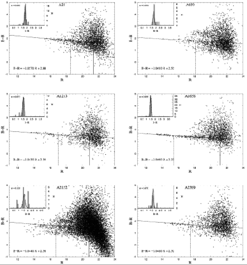
Figure 1.—

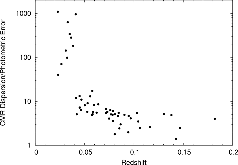
Figure 2.—

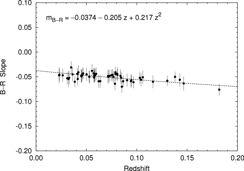
Figure 3.—

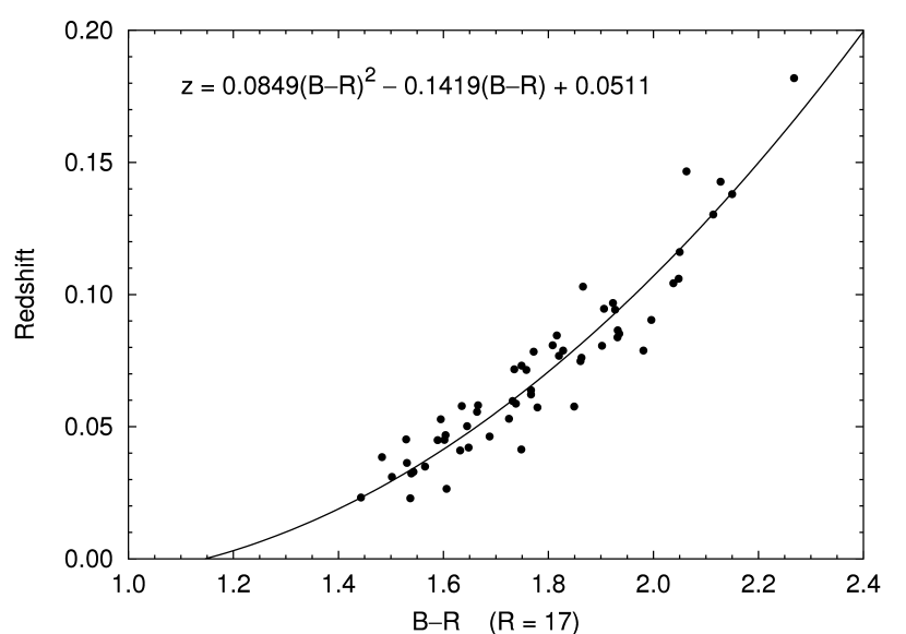
Figure 4.—

Table 1Cluster Sample and CMR Fits

Cluster	Redshift($z$)	Slope (b)	Zero Point (a)	$\sigma_{CMR}$	$(B-R)_{R=17}$
A21	0.0946	-0.057 $\pm$ 0.012	2.88 $\pm$ 0.20	0.080	1.91
A84	0.1030	-0.052 $\pm$ 0.013	2.75 $\pm$ 0.21	0.097	1.87
A85	0.0556	-0.038 $\pm$ 0.014	2.31 $\pm$ 0.22	0.113	1.66
A98	0.1043	-0.056 $\pm$ 0.013	2.99 $\pm$ 0.22	0.077	2.04
A154	0.0638	-0.059 $\pm$ 0.013	2.77 $\pm$ 0.22	0.115	1.77
A168	0.0452	-0.048 $\pm$ 0.013	2.34 $\pm$ 0.20	0.042	1.53
A260	0.0363	-0.045 $\pm$ 0.014	2.30 $\pm$ 0.22	0.093	1.53
A399	0.0715	-0.048 $\pm$ 0.013	2.58 $\pm$ 0.22	0.088	1.76
A401	0.0748	-0.047 $\pm$ 0.012	2.66 $\pm$ 0.19	0.062	1.86
A407	0.0463	-0.046 $\pm$ 0.013	2.47 $\pm$ 0.21	0.072	1.69
A415	0.0788	-0.044 $\pm$ 0.013	2.74 $\pm$ 0.23	0.055	1.98
A496	0.0329	-0.052 $\pm$ 0.013	2.43 $\pm$ 0.22	0.063	1.54
A514	0.0731	-0.048 $\pm$ 0.013	2.56 $\pm$ 0.21	0.075	1.75
A629	0.1380	-0.050 $\pm$ 0.010	3.00 $\pm$ 0.19	0.112	2.15
A634	0.0265	-0.047 $\pm$ 0.014	2.40 $\pm$ 0.22	0.028	1.61
A646	0.1303	-0.058 $\pm$ 0.010	3.10 $\pm$ 0.18	0.130	2.11
A665	0.1819	-0.076 $\pm$ 0.012	3.56 $\pm$ 0.21	0.145	2.27
A671	0.0502	-0.045 $\pm$ 0.014	2.41 $\pm$ 0.22	0.070	1.64
A690	0.0788	-0.041 $\pm$ 0.011	2.52 $\pm$ 0.19	0.091	1.83
A779	0.0229	-0.047 $\pm$ 0.016	2.34 $\pm$ 0.24	0.109	1.54
A957	0.0450	-0.049 $\pm$ 0.013	2.44 $\pm$ 0.21	0.061	1.60
A999	0.0323	-0.054 $\pm$ 0.017	2.46 $\pm$ 0.24	0.085	1.54
A1142	0.0349	-0.031 $\pm$ 0.013	2.09 $\pm$ 0.22	0.034	1.56
A1213	0.0468	-0.043 $\pm$ 0.012	2.34 $\pm$ 0.19	0.073	1.60
A1291	0.0530	-0.050 $\pm$ 0.012	2.58 $\pm$ 0.21	0.077	1.72
A1413	0.1427	-0.056 $\pm$ 0.013	3.08 $\pm$ 0.23	0.076	2.13
A1569	0.0784	-0.064 $\pm$ 0.013	2.86 $\pm$ 0.22	0.067	1.77
A1650	0.0845	-0.052 $\pm$ 0.012	2.70 $\pm$ 0.22	0.084	1.82
A1656	0.0232	-0.046 $\pm$ 0.012	2.22 $\pm$ 0.21	0.056	1.44
A1775	0.0717	-0.050 $\pm$ 0.014	2.58 $\pm$ 0.24	0.071	1.74
A1795	0.0622	-0.059 $\pm$ 0.013	2.77 $\pm$ 0.23	0.067	1.77
A1913	0.0528	-0.050 $\pm$ 0.013	2.44 $\pm$ 0.21	0.047	1.60
A1983	0.0449	-0.048 $\pm$ 0.013	2.40 $\pm$ 0.22	0.062	1.59
A2022	0.0578	-0.048 $\pm$ 0.013	2.45 $\pm$ 0.22	0.070	1.64
A2029	0.0768	-0.050 $\pm$ 0.012	2.67 $\pm$ 0.20	0.080	1.82
A2152	0.0410	-0.044 $\pm$ 0.011	2.38 $\pm$ 0.20	0.126	1.63
A2244	0.0968	-0.061 $\pm$ 0.012	2.96 $\pm$ 0.21	0.073	1.92
A2247	0.0385	-0.060 $\pm$ 0.011	2.50 $\pm$ 0.18	0.032	1.48
A2255	0.0808	-0.046 $\pm$ 0.012	2.59 $\pm$ 0.20	0.073	1.81
A2256	0.0581	-0.047 $\pm$ 0.013	2.46 $\pm$ 0.22	0.050	1.67
A2271	0.0576	-0.051 $\pm$ 0.012	2.72 $\pm$ 0.20	0.059	1.85
A2328	0.1466	-0.063 $\pm$ 0.014	3.14 $\pm$ 0.23	0.130	2.06
A2356	0.1161	-0.060 $\pm$ 0.013	3.07 $\pm$ 0.24	0.061	2.05
A2384	0.0943	-0.059 $\pm$ 0.013	2.93 $\pm$ 0.23	0.046	1.93
A2399	0.0587	-0.046 $\pm$ 0.013	2.52 $\pm$ 0.22	0.070	1.74
A2410	0.0806	-0.044 $\pm$ 0.014	2.65 $\pm$ 0.24	0.031	1.90
A2415	0.0597	-0.044 $\pm$ 0.013	2.48 $\pm$ 0.23	0.089	1.73
A2420	0.0838	-0.048 $\pm$ 0.013	2.75 $\pm$ 0.23	0.078	1.93
A2440	0.0904	-0.057 $\pm$ 0.013	2.96 $\pm$ 0.23	0.088	2.00
A2554	0.1060	-0.051 $\pm$ 0.014	2.92 $\pm$ 0.23	0.052	2.05
A2556	0.0865	-0.059 $\pm$ 0.012	2.94 $\pm$ 0.21	0.049	1.93
A2593	0.0421	-0.041 $\pm$ 0.014	2.34 $\pm$ 0.23	0.048	1.65
A2597	0.0852	-0.070 $\pm$ 0.012	3.12 $\pm$ 0.24	0.037	1.94
A2626	0.0573	-0.043 $\pm$ 0.012	2.51 $\pm$ 0.20	0.059	1.78
A2634	0.0310	-0.053 $\pm$ 0.013	2.40 $\pm$ 0.20	0.047	1.50
A2657	0.0414	-0.054 $\pm$ 0.013	2.68 $\pm$ 0.21	0.077	1.75
A2670	0.0761	-0.046 $\pm$ 0.012	2.64 $\pm$ 0.20	0.094	1.86

References

- Aaronson, Persson, & Frogel (1981) Aaronson, M., Persson, S.E., & Frogel, J.A. 1981, ApJ, 245, 18
- Aragón-Salamanca et al. (1993) Aragón-Salamanca, A., Ellis, R.S., Couch, W.J., & Carter, D. 1993, MNRAS, 262, 764
- Arimoto & Yoshii (1987) Arimoto, N., & Yoshii, Y. 1987, A&A, 173, 23
- Baade (1944) Baade, W. 1944, ApJ, 100, 137
- Babu & Rao (1993) Babu, G.J., & Rao, C.R. 1993, in Handbook of Statistics, Vol. 9, ed. C.R. Rao (Amsterdam: Elsevier Science), 627
- Babu & Singh (1983) Babu, G.J., & Singh, K. 1983, Annals Statist., 11, 999
- Barkhouse (2003) Barkhouse, W.A. 2003, Ph.D. Thesis, University of Toronto
- Baum (1959) Baum, W.A. 1959, PASP, 71, 106
- Beers, Flynn, & Gebhardt (1990) Beers, T.C., Flynn, K., & Gebhardt, K. 1990, AJ, 100, 32
- Biviano et al. (1995) Biviano , A., Durret , F., Gerbal , D., Le Fevre , O., Lobo , C., Mazure , A. & Slezak , E. 1995, A&A, 297, 610
- Blakeslee (2001) Blakeslee, J.P. 2001, in Proceedings of the STScI Symp., The Dark Universe: Matter, Energy, and Gravity, ed. M. Livio, preprint (astro-ph/0108253)
- Blakeslee et al. (2003) Blakeslee, J.P., Franx, M., Postman, M., et al. 2003, ApJ, 596, L143
- Bloomfield & Steiger (1983) Bloomfield, P., & Steiger W.L 1983, in Progress in Probability and Statistics, Vol. 8, ed. P. Huber, & M. Rosenblatt (Boston: Birkhäuser)
- Bower, Lucey, & Ellis (1992) Bower, R.G., Lucey, J.R., & Ellis, R.S. 1992, MNRAS, 254, 601 (BLE)
- Bower et al. (1998) Bower, R.G., Terlevich, A., Kodama, T., & Caldwell, N. 1998, ASP Conf. Ser. 163, Star Formation in Early Type Galaxies, ed. P. Carral, & J. Cepa (San Francisco: ASP), 211
- Brown (1997) Brown, J.P. 1997, Ph.D. Thesis, University of Toronto
- Brunner et al. (1997) Brunner, R.J., Connolly, A., Szalay, A.S., & Bershady, M.A. 1997, ApJ, 482, L21
- Burstein & Heiles (1982) Burstein, D., & Heiles, C. 1982, AJ, 87, 1165
- Burstein & Heiles (1984) Burstein, D., & Heiles, C. 1984, ApJS, 54, 33
- Butcher & Oemler (1984) Butcher, H., & Oemler A. 1984, ApJ, 285, 426
- Carlberg (1984) Carlberg, R.G. 1984, ApJ, 286, 403
- Cole & Lacey (1996) Cole, S., & Lacey, C. 1996, MNRAS, 281, 716
- Coleman, Wu, & Weedman (1980) Coleman, G.D., Wu, C.C., & Weedman, D.W. 1980, ApJS, 43, 393
- de Jong (1996) de Jong, R.S. 1996, A&A, 133, 377
- Dixon, Godwin, & Peach (1989) Dixon, K.L., Godwin, J.G., & Peach, J.V. 1989, MNRAS, 239, 459
- Dressler (1978) Dressler, A. 1978, ApJ, 223, 765
- Dressler (1980) Dressler, A. 1980, ApJ, 236, 351
- Dressler (1984) Dressler, A. 1984, ARA&A, 22, 185
- Ebeling et al. (1996) Ebeling, H., Voges, W., Bohringer, H., Edge, A.C., Huchra, J.P., & Briel, U.G. 1996, MNRAS, 281, 799
- Efron & Tibshirani (1986) Efron, B., & Tibshirani, R. 1986, Statistical Sci., 1, 54
- Ellis et al. (1997) Ellis, R.S., Smail, I., Dressler, A., Couch, W.J., Oemler, A., Butcher, H., & Sharples R.M. 1997, ApJ, 483, 582
- Ferreras, Charlot, & Silk (1999) Ferreras, I., Charlot, S., & Silk, J. 1999, ApJ, 521, 81
- Fowler & Greenstein (1956) Fowler, W.A., & Greenstein, J.L. 1956, Proc. Nat. Acad. Sci., 42, 173
- Gadotti & dos Anjos (2001) Gadotti, D.A., & dos Anjos, S. 2001, AJ, 122, 1298
- Garilli et al. (1996) Garilli, B., Bottini, D., Maccagni, D., Carrasco, L., & Recillas, E. 1996, ApJS, 105, 191
- Gladders et al. (1998) Gladders, M.D., López-Cruz, O., Yee, H.K.C., & Kodama, T. 1998, ApJ, 501, 571
- Gladders & Yee (2000) Gladders, M.D., & Yee, H.K.C. 2000, AJ, 120, 2148
- Govoni et al. (2001) Govoni, F., Taylor, G.B., Dallacasa, D., Feretti, L., & Giovannini, G. 2001, A&A, 379, 807
- Hausman & Ostriker (1978) Hausman, M.A., & Ostriker, J.P. 1978, ApJ, 224, 320
- Jones & Forman (1999) Jones, C., & Forman, W. 1999, ApJ, 511, 65
- Kauffmann & Charlot (1998) Kauffmann, G., & Charlot, S. 1998, MNRAS, 294, 705
- Kodama (1997) Kodama, T. 1997, Ph.D. Thesis, University of Tokyo
- Kodama & Arimoto (1997) Kodama, T., & Arimoto, N. 1997, A&A, 321, 41 (KA)
- Kolokotronis et al. (2001) Kolokotronis, V., Basilakos, S., Plionis, M., & Georgantopoulos, I. 2001, MNRAS, 320, 49
- Kormendy & Djorgovski (1989) Kormendy, J., & Djorgovski, S.G. 1989, ARA&A, 27, 235
- Landolt (1992) Landolt, A.U. 1992, AJ, 104, 372
- Larson (1974a) Larson, R.B. 1974a, MNRAS, 166, 585
- Larson (1974b) Larson, R.B. 1974b, MNRAS, 169, 229
- López-Cruz (1997) López-Cruz O. 1997, Ph.D. Thesis, University of Toronto
- López-Cruz (2001) López-Cruz, O. 2001, Rev. Mex. Astron. Astrophys, Conf. Ser., 11, 183
- López-Cruz (2003) López-Cruz, O. 2003, in The Garrison Festschrift, eds. R.O. Gray, C. Corbally, & A.G. Davis Philip, (Schenectady: L Davis Press, Inc.), 109
- López-Cruz et al. (1997) López-Cruz, O., Yee, H.K.C., Brown, J.P., Jones. C., & Forman, W. 1997, ApJ, 475, L97
- López-Cruz et al. (2002) López-Cruz, O., Schade, D., Barrientos, et al. 2002, in New Quests in Stellar Astrophysics: The Link between Stars and Cosmology, eds. M. Chávez et al. (Dordrecht:Kluwer Academic Publisher), 269
- Metcalfe et al. (1994) Metcalfe, N., Godwin, J.G., & Peach, J.V. 1994, MNRAS, 267, 431
- Odell, Schombert, & Rakos (2002) Odell, A. P., Schombert, J. & Rakos, K. 2002, AJ, 124, 3061
- Pahre et al. (1996) Pahre, M.A., Djorgovski, S.G., & De Carvalho, R.R. 1996, ApJ, 456, L79
- Peebles (2002) Peebles, P. J. E. 2002, ASP Conf. Ser., 283, A New Era in Cosmology, eds. N. Metcalfe & T. Shanks (San Francisco, ASP), 351
- Peletier et al. (1990) Peletier, R.F., Davies, R.L., Davis, L.E., Illingworth, G.D., & Cawson, M. 1990, AJ, 100, 1091
- Pimbblet et al. (2002) Pimbblet, K.A., Smail, I., Kodama, T., Couch, W.J., Edge, A.C., Zabludoff, A.I., O’Hely, E. 2002, MNRAS, 331, 333
- Postman & Lauer (1995) Postman, M., & Lauer, T.R. 1995, ApJ, 440, 28
- Press et al. (1992) Press, W.H., Teukolsky, S.A., Vetterling, W.T., & Flannery, B.P. 1992, Numerical Recipes, The Art of Scientific Computing, (2d ed.; Cambridge, Cambridge University Press)
- Rey (1980) Rey, W. 1980, Introduction to Robust and Quasi-Robust Statistical Methods, (Springer-Verlag: Berlin)
- Roouseeuw & Leroy (1987) Roouseeuw, R.J., & Leroy, A.M. 1987, Robust Regression and Outlier Detection, (Wiley: New York)
- Sandage (1972) Sandage, A. 1972, ApJ, 176, 21
- Sandage & Visvanathan (1978a) Sandage, A., & Visvanathan, N. 1978a, ApJ, 223, 707
- Sandage & Visvanathan (1978b) Sandage, A., & Visvanathan, N. 1978b, ApJ, 228, 81
- Schlegel, Finkbeiner, & Davis (1998) Schlegel, D. J., Finkbeiner, D. P. & Davis, M. 1998, ApJ, 500, 525
- Secker, Harris, & Plummer (1998) Secker, J., Harris, W.E., & Plummer, J.D. 1998, PASP, 109, 1364
- Spergel et al. (2003) Spergel, D. N, Verde, L., Peiris, H. V., et al., 2003, ApJS, 148, 175
- Stanford, Eisenhardt, & Dickinson (1998) Stanford, S.A., Eisenhardt, P.R., & Dickinson, M. 1998, ApJ, 492, 461
- Struve (1956) Struve, O. 1956, S&T, 15, 391
- Taylor et al. (2003) Taylor, V.A., Odewahn, S.C., Jansen, R.A., Windhorst, R.A., Hibbard, J.E. 2003, abstract, AAS Meeting 203, #146.04
- Terlevich, Caldwell, & Bower (2001) Terlevich, A. I., Caldwell, N. & Bower, R. G. 2001, MNRAS, 326, 1547
- Thompson & Gregory (1993) Thompson, L.A., & Gregory, S.A. 1993, AJ, 106, 2197
- van Dokkum et al. (1998) van Dokkum, P.G, Franx, M., Kelson, D.D., Illingworth, G.D., Fisher, D., & Fabricant, D. 1998, ApJ, 500, 714
- van Dokkum et al. (2001) van Dokkum, P.G., Stanford, S.A., Holden, B.P., Eisenhardt, P.R., Dickson, M., & Elston, R. 2001, ApJ, 552, 101
- Vazdekis et al. (2001) Vazdekis, A., Kuntschner, H., Davies, R.L., Arimoto, N., Nakamura, O., & Peletier, R. 2001, ApJ, 551, 127
- Visvanathan & Sandage (1977) Visvanathan, N., & Sandage, A. 1977, ApJ, 216, 214
- Yee (1991) Yee, H.K.C. 1991, PASP, 103, 396
- Yee (1999) Yee, H.K.C. 1999, in the proceedings of the Xth Rencontres de Blois on “The Birth of Galaxies”, eds. Guiderdoni & Thuan, in press (astro-ph/9809347).
- Yee et al. (1996) Yee, H.K.C., Ellingson, E., Abraham, R.G., Gravel, P., Carlberg, R.G., Smecker-Hane, T.A., Schade, D., & Rigler, M. 1996, ApJS, 102, 289
- Yee, Ellingson, & Carlberg (1996) Yee, H.K.C., Ellingson, E., & Carlberg, R.G. 1996, ApJS, 102, 269
- Yee & López-Cruz (1999) Yee, H.K.C., & López-Cruz, O. 1999, AJ, 117, 1985
- Yee & Ellingson (2003) Yee, H. K. C. & Ellingson, E. 2003, ApJ, 585,215
- Worthey et al. (1995) Worthey, G., Trager, S., & Faber, S.M. 1995, in ASP Conf. Ser. 86, Fresh Views of Elliptical Galaxies, ed. A. Buzzoni, A. Renzini, & A. Serrano, (San rFrancisco: ASP), 203
- Wu et al. (2004) Wu, H., Shao, Z., Mo, H.J., Xia, X., & Deng, Z. 2004, preprint (astro-ph/0404226)