T Dwarfs and the Substellar Mass Function. I. Monte Carlo Simulations

Abstract

Monte Carlo simulations of the field substellar mass function (MF) are presented, based on the latest brown dwarf evolutionary models from Burrows et al. (1997) and Baraffe et al. (2003). Starting from various representations of the MF below 0.1 M_☉ and the stellar birth rate, luminosity functions (LFs) and T_eff distributions are produced for comparison with observed samples. These distributions exhibit distinct minima in the mid-type L dwarf regime followed by a rise in number density for fainter/cooler brown dwarfs, predicting many more T-type and cooler brown dwarfs in the field even for relatively shallow mass functions. Deuterium-burning brown dwarfs (0.012 M_☉ $\leq$ M $\leq$ 0.075 M_☉) dominate field objects with 400 $\leq$ T_eff $\leq$ 2000 K, while non-fusing brown dwarfs make up a substantial proportion of field dwarfs with T_eff $\leq$ 500 K. The shape of the substellar LF is fairly consistent for various assumptions of the Galactic birth rate, choice of evolutionary model, and adopted age and mass ranges, particularly for field T dwarfs, which as a population provide the best constraints for the field substellar MF. Exceptions include a depletion of objects with 1200 $\leq$ T_eff $\leq$ 2000 K in “halo” systems (ages $>$ 9 Gyr), and a substantial increase in the number of very cool brown dwarfs for lower minimum formation masses. Unresolved multiple systems tend to enhance features in the observed LF and may contribute significantly to the space density of very cool brown dwarfs. However, these effects are small ($<$ 10% for T${}_{eff}\lesssim 300$ K) for binary fractions typical for brown dwarf systems (10–20%). An analytic approximation to correct the observed space density for unresolved multiple systems in a magnitude-limited survey is derived. As an exercise, surface densities as a function of T_eff are computed for shallow near-infrared (e.g., 2MASS) and deep red-optical (e.g., UDF) surveys based on the simulated LFs and empirical absolute magnitude/T_eff relations. These calculations indicate that a handful of L and T dwarfs, as well as late-type M and L halo subdwarfs, should be present in the UDF field depending on the underlying MF and disk scale height. These simulations and their dependencies on various factors provide a means for extracting the field substellar MF from observed samples, an issue pursued using 2MASS T dwarf discoveries in Paper II.

1 Introduction

The stellar Initial Mass Function (IMF) is a fundamental quantity in astrophysics. Defined as the total number density of stars ever created in a particular environment per unit mass (Miller & Scalo, 1979), the IMF is a sensitive probe of the star formation process, accounts for the mass budget and evolution of galaxies, and determines the evolution of chemical abundances over time. Pioneering work by Salpeter (1955) showed that the IMF for field stars in the Solar Neighborhood (masses $0.4\lesssim$ M $\lesssim 10$ M_☉) could be adequately reproduced by a power law, $\Psi$(M) $\equiv$ $\frac{dN}{dM}$ $\propto$ M^-2.35, a result that generally persists to this day (Scalo, 1998; Kroupa, 2001; Reid, Gizis, & Hawley, 2002). Since that time, many studies of the IMF have been undertaken for low and high mass stars of differing populations, and in various regions of the Galaxy and external star clusters. Excellent reviews can be found in Miller & Scalo (1979); Scalo (1986); Kroupa (1998); Scalo (1998); Reid & Hawley (2000); and Chabrier (2003).

The IMF is a particularly key measurement in the study of brown dwarfs. These objects comprise the low-mass tail of the stellar population, but differ in that they lack sufficient mass to sustain core Hydrogen fusion (Hayashi & Nakano, 1963; Kumar, 1963). Because of this, brown dwarfs never reach the Hydrogen main sequence, but instead continually evolve to cooler temperatures and fainter magnitudes. The intrinsic faintness of brown dwarfs made them an early candidate for dark matter (Tarter, 1975; Bahcall, 1984); indeed, an extrapolation of the Salpeter IMF yields nearly twice as much mass in brown dwarfs (0.005 $\lesssim$ M $\lesssim$ 0.075 M_☉) as in stars (0.075 $\lesssim$ M $\lesssim$ 40 M_☉). However, number counts of field M dwarfs show a flattening in the IMF around 0.3–0.5 M_☉ (Sandage, 1957; Schmidt, 1959; Miller & Scalo, 1979), and it is now quite clear that brown dwarfs are not prolific enough to be the constituents of dark matter. Nevertheless, the number density of brown dwarfs may still be a significant fraction or multiple of the stellar density (Reid et al., 1999; Kroupa, 2001; Chabrier, 2002), and the nearest systems to the Sun may in fact be unidentified substellar ones. Furthermore, quantifying the IMF in the substellar regime enables a unique exploration of the star formation process; in particular, its efficiency at small masses and the lower limit at which self-gravitating “stars” can form.

The IMF is not an observable quantity, and is generally derived from the Luminosity Function (LF), $\Phi(M_{bol})$, the number density of stars observed in a defined region per unit luminosity. The LF is converted into the Present Day Mass Function (PDMF, the number density of stars currently present in a defined region per unit mass), using empirical (e.g., Henry & McCarthy 1993) or theoretical (e.g., Baraffe et al. 1998) mass-luminosity (M-L) relations. For the lowest-mass stars and brown dwarfs (M $\lesssim 0.1$ M_☉) in well-defined regions of space, and assuming no evolution of the star-forming process over time (although its rate can change), the IMF is identical to the PDMF and can be referred to simply as the Mass Function (MF).

While this technique is suitable for low-mass stellar populations, substellar MF determinations are hindered by their thermal evolution. A brown dwarf with an observed luminosity and/or effective temperature (T_eff) has a wide range of possible masses depending on its age. This mass-age degeneracy is not critical for young cluster brown dwarf populations, where members are assumed to be approximately coeval (e.g., White & Ghez 2001). In the Galactic disk, however, stars and brown dwarfs can span a fairly broad range of ages, from a few tens of Myr to $\sim$ 10 Gyr. In other words, there is no single M-L relation that can be used to convert the LF into the MF for brown dwarfs in the field. Field brown dwarfs are also generally older than their young cluster counterparts, so that the lowest mass field objects can be exceedingly faint, requiring deep and/or wide area surveys to detect sufficient numbers. Nevertheless, the physical properties of evolved brown dwarfs are better understood than their younger counterparts, without the complications of youthful accretion or rapid evolution. Furthermore, the nearby population of stars is not affected by reddening; can be more easily followed-up with spectroscopic, parallactic, and high-resolution imaging observations (to derive physical characteristics and multiplicity); and, assuming that it is well-mixed, is generally devoid of foreground or background contamination.

This article is the first of a two-part series investigating the substellar MF in the Solar Neighborhood, by comparing simulated LFs to a magnitude-limited sample of T dwarfs (Burgasser et al., 2003a) identified in the Two Micron All Sky Survey (Cutri et al., 2003, hereafter 2MASS). T dwarfs are a spectroscopic class of brown dwarfs that exhibit CH₄ absorption (Burgasser et al., 2002b; Geballe et al., 2002), implying T${}_{eff}\lesssim 1300$ K (Kirkpatrick et al., 2000; Golimowski et al., 2004). In this article, Monte Carlo simulations of the field substellar MF are examined, and dependencies on various input parameters are investigated. These simulations are comparable to those of Allen et al. (2004), who constrain the substellar MF through Bayesian techniques. The implementation of the simulations presented here is described in $\S$ 2, which includes discussion of the various input distributions and evolutionary models used. An in-depth analysis of the derived LF and T_eff distributions and their features is given in $\S$ 3. In $\S$ 4, the sensitivity of these distributions between the evolutionary models employed, different birth rates, different age and mass limits, and the influence of unresolved multiple systems is explored. Surface density predictions based on the simulations are derived for both shallow and deep magnitude-limited surveys in $\S$ 5. Results are summarized in $\S$ 6.

2 The Simulations

2.1 General Description of the Problem

The purpose of these simulations is to create a statistical link between the MF and LF, or more generally a link between the fundamental properties of brown dwarfs – mass, age, and metallicity – and their observables – T_eff and luminosity. This link is made through evolutionary models coupled to non-grey model atmospheres. In this study, we assume that all brown dwarfs are described by a single distribution for each of their fundamental parameters, denoted $P(x)$, where $x$ is the fundamental property in question. The fundamental distributions examined are summarized in Table 1 and described in detail below.

Following traditional practice, it is assumed that the MF does not evolve with time, so that the number density of stars ever created per unit mass and per unit time, $C({\rm M},t)$ (termed the Creation Function by Miller & Scalo 1979) can be separated into mass- and time-dependent functions:

$$C({\rm M},t)=\Psi({\rm M}){\times}b(t)/T_{o}$$ (1)

(Miller & Scalo, 1979), where $\Psi({\rm M})$ is the MF, $b(t)$ is the birth rate (number density of stars born per unit time), and $T_{o}$ is the age of the Galaxy, assumed here to be 10 Gyr. The separation of $C({\rm M},t)$ enables the examination of the MF and birth rates separately. The metallicity ($Z$) and mass ratio ($q$) distributions are also assumed to be independent so that they may be treated separately as well. Clearly, these assumptions may not accurately reflect the detailed stellar formation history of the Galaxy (e.g., chemical evolution is ignored; see Edvardsson et al. 1993), but are adequate for current substellar MF determinations.

2.2 Fundamental Distributions

2.2.1 The Mass Distribution

Six MFs were examined, including five power-law distributions:

$$\Psi({\rm M})\propto{\rm M}^{-{\alpha}}$$ (2)

with $\alpha$ = 0.0, 0.5, 1.0, 1.5, and 2.0; and the lognormal MF from Chabrier (2001):

$$\Psi({\rm\log{M}})\propto e^{-\frac{({\rm\log{M}}-{\rm\log{M_{c}}})^{2}}{2{\sigma}^{2}}}$$ (3)

(see also Miller & Scalo 1979), where M_c = 0.1 M_☉ and $\sigma$ = 0.627. Note that $\Psi$(${\rm\log{M}}$) = $\ln{10}$ M $\Psi$(M). The baseline simulations incorporate a mass range 0.01 $\leq$ M $\leq$ 0.1 M_☉, with the upper limit set by the evolutionary models and the lower limit set to provide enough objects in the higher mass bins, particularly for the steeper power laws. Lower mass limits ranging from 0.001 to 0.015 M_☉ were also examined in order to measure the influence of a minimum “cut-off” mass (M_min) in brown dwarf formation ($\S$ 4.2.4).

2.2.2 The Age Distribution

The age distribution is related to the birth rate by $P(t)=b(T_{o}-t)$. The birth rate does not influence the shape of the MF if the latter is assumed not to evolve. However, as brown dwarfs themselves evolve thermally, the age distribution can influence the LF. Five birth rates were examined, as illustrated in Figure 1:

$$P(t)=b_{1}(T_{o}-t)=1,$$ (4)

$$P(t)=b_{2}(T_{o}-t)\propto{\rm e}^{-(T_{o}-t)/{\tau}_{g}},$$ (5)

$$P(t)=b_{3}(T_{o}-t)=\left\{\begin{array}[]{ll}1.1&0\leq t<1~{}{\rm Gyr}\\ 0.5&1\leq t<2~{}{\rm Gyr}\\ 1.3&2\leq t<5~{}{\rm Gyr}\\ 0.8&5\leq t<7~{}{\rm Gyr}\\ 1.1&7\leq t<9~{}{\rm Gyr}\\ 0.8&9\leq t<10~{}{\rm Gyr}\\ \end{array}\right.$$ (6)

$$P(t)=b_{4}(T_{o}-t)\propto\sum_{i=1}^{N_{cl}}{{\rm e}^{-\frac{((T_{o}-t)-t_{o}^{i})^{2}}{2{\tau}_{cl}^{2}}}},$$ (7)

and

$$P(t)=b_{5}(T_{o}-t)=\left\{\begin{array}[]{ll}10&0\leq t\leq 1~{}{\rm Gyr}\\ 0&t>1~{}{\rm Gyr}\\ \end{array}\right..$$ (8)

The first (“constant”) birth rate is the simplest and most frequently employed for MF simulations, and a number of authors have asserted its legitimacy based on studies of the Galactic star formation history (SFH). Miller & Scalo (1979) argue that the SFH must be roughly flat over the age of the Galaxy to explain the continuity of the MF between low and high mass stars; formation rates, kinematics, and spatial distribution of planetary nebulae and white dwarfs; nucleosynthesis yields; distribution of H II regions; and theoretical predictions at that time. Soderblom, Duncan, & Johnson (1991) claim no evidence of variation of the star formation rate over the past 10⁹ years based on the activity distribution of G and K stars, (although a reanalysis by Rocha-Pinto & Maciel (1998) argues otherwise; see below). Boissier & Prantzos (1999) also find little evidence for variation between recent and early SFHs based on the metallicity distribution of G-dwarfs.

The second (“exponential”) birth rate has been used to model Galactic star formation (Tinsley, 1974; Miller & Scalo, 1979) because of its simple form. This birthrate is consistent with a star formation rate that scales with the average gas density (Miller & Scalo, 1979), with an e-folding time ${\tau}_{g}$ = 5 Myr; i.e., half of the age of the Galaxy (as adopted here). Miller & Scalo (1979) find this rate to be marginally consistent with continuity arguments, although in general there are no empirical data that strongly support this function.

More recent studies have suggested that the SFH is not strictly monotonic, but can be characterized by a series of burst events. Barry (1988) point out an apparent increase in star formation 400 Myr ago, a result supported by an examination of the white dwarf luminosity function by Noh & Scalo (1990, however, see Soderblom, Duncan, & Johnson 1991). The presence of perhaps three burst episodes in the SFH of the Galaxy is detailed in Majewski (1993). To model such a non-monotonic birth rate, a smoothed version of the empirical results of Rocha-Pinto et al. (2000) was used, based on the chromospheric ages of late-type dwarfs. This “empirical” birth rate exhibits peaks 0–1, 2–5, and 7–9 Gyr ago, with somewhat lower formation rates in between these bursts. As discussed in Rocha-Pinto et al. (2000), a smoothed distribution may hide more dramatic swings in the Galactic SFH, but the detection of such events are hindered by uncertainties in stellar age measurements. Note that this non-monotonic birth rate does not violate the continuity arguments of Miller & Scalo (1979).

The fourth birth rate examined is a novel one assuming star formation has occurred entirely in young clusters, in a series of short-lived formation bursts evenly and randomly distributed over the age of the Galaxy. The formation period is short in young clusters, ${\tau}_{cl}\approx 10-20$ Myr (White & Ghez, 2001), so that this birth rate approximates a “stochastic” formation process. A total of $N_{cl}=50$ clusters was assumed, randomly distributed over the age of the Galaxy and each producing an equal number of brown dwarfs over the same formation timescale. The birth rate distribution of each cluster was assumed to be Gaussian with a characteristic time scale ${\tau}_{cl}=10$ Myr. These assumptions are not necessarily representative of the true yields and lifetimes of young clusters in the Galaxy, but are suitable for this study.

Finally, the fifth (“halo”) birth rate considers only brown dwarfs born within a 1 Gyr burst 9 Gyr in the past, and is meant to represent the conditions of the Galactic halo or old globular cluster substellar populations (Reid & Hawley, 2000).

For each of these birth rates, an age range of $0.01\leq t\leq 10$ Gyr is nominally adopted, although minimum ages of 1 to 100 Myr were also examined to investigate the contribution of young populations in the simulated LFs (see $\S$ 4.2.3).

2.2.3 The Metallicity Distribution

The choice of a metallicity distribution is primarily constrained by the evolutionary models used ($\S$ 2.3), both of which assume solar abundances. Therefore, a constant distribution $P(Z)$ = 1 is adopted with $Z=Z_{\sun}$. This choice is supported by the fact that 70% of disk stars have abundances $-0.3<[m/H]<0.15$ (Reid & Hawley, 2000), but requires that there is no significant contamination by other Galactic populations (e.g., thick disk and halo brown dwarfs) in the observed sample.

2.3 Evolutionary Models

To convert our fundamental properties to observables, we used the most recent evolutionary calculations from the Tucson (Burrows et al., 1997) and Lyon (Baraffe et al., 2003) groups. Both of these models employ non-grey atmospheres in which condensate opacity is ignored (so-called “COND” models; Allard et al. 2001), largely consistent with the observed spectra of mid-type M and mid- and late-type T dwarfs (Tsuji, Ohnaka, & Aoki, 1996). Chabrier et al. (2000a) have also derived evolutionary tracks for “DUSTY” atmosphere models, which retain condensate material in their atmosphere, more appropriate for warmer late-type M and L dwarfs (Tsuji, Ohnaka, & Aoki, 1996). However, these authors find $\lesssim$10% difference in the evolution of luminosity and T_eff between the COND and DUSTY models. This is a relatively small deviation given the potentially larger systematic uncertainties arising from the complex evolution of condensates in cool M and L dwarf atmospheres (Ackerman & Marley, 2001; Burgasser et al., 2002a; Tsuji, 2002; Cooper et al., 2003) and current observational uncertainties (Burgasser, 2001; Cruz et al., 2003). DUSTY evolutionary tracks are therefore ignored in this investigation.

In Figure 1, the evolution of T_eff with time for the two sets of models employed are compared for masses 0.001 $\leq$ M $\leq$ 0.1 M_☉ and ages 1 Myr to 10 Gyr. Over much of this parameter space evolutionary tracks are consistent to within 10%, with the Baraffe models predicting slightly higher temperatures at a particular mass and age for M $<$ 0.06 M_☉ and lower temperatures for M $>$ 0.08 M_☉. At early ages ($t\lesssim 5$ Myr) the Burrows models are significantly hotter (20–25%) for M $>$ 0.06 M_☉. At later ages ($t\gtrsim 5$ Gyr), the two models again deviate significantly (20–35%) for 0.06 $\lesssim$ M $\lesssim$ 0.08 M_☉, with the Baraffe models being both hotter and more luminous. This is due to the higher Hydrogen Burning Minimum Mass (HBMM) for the Burrows models, 0.075 versus 0.072 M_☉. Finally, the Burrows tracks diverge more substantially around the HBMM, with a difference of 1500 K between 0.075 and 0.09 M_☉ at 10 Gyr, as compared to 600 K for identical masses and ages in the Baraffe models. The effects of these differences on the simulated LFs are described in $\S$ 4.2.1.

2.4 Implementation of the Simulations

For each simulation, a total of $3{\times}10^{6}$ objects were assigned a set of fundamental properties $x_{i}$ ($x$ = M, $t$) by selecting the random parameter ${\xi}_{i}$ from a uniform distribution over the range:,

$${\xi}_{i}~{}{\epsilon}~{}[{\rm min}(\bar{P}\{x\}),{\rm max}(\bar{P}\{x\})],$$ (9)

where

$$\{x\}~{}{\epsilon}~{}[x_{min},x_{max}]$$ (10)

and

$$\bar{P}(x)\propto\int{P}(x)dx;$$ (11)

so that

$$x_{i}=\bar{P}^{-1}({\xi}_{i}).$$ (12)

Each object was then assigned a luminosity (and hence $M_{bol}=-2.5\log{(L/L_{\sun})}+4.74$; Livingston 2000) and T_eff by linearly interpolating the grid points of the appropriate evolutionary model to that object’s mass and logarithmic age. Minimum values of $M_{bol}$ = 50 mag and $T_{eff}$ = 100 K were assigned to the derived observables if the model values fell below these limits. The observable distributions $\Phi(M_{bol})$ (in units of pc^-3 mag^-1) and $\Phi({\rm T}_{eff})$ (in units of pc^-3 [100 K]^-1) were then determined by binning the observable parameters every 0.5 mag and 100 K, respectively.

In order to extract meaningful comparisons between the various distributions and empirical data, simulated MF number densities were normalized to the mean of the field low-mass star (0.1–1.0 M_☉) MFs of Reid et al. (1999) and Chabrier (2001), $\Psi$(M) = $0.35(\frac{\rm M}{0.1{\rm M}_{\sun}})^{-1.13}$ and $\Psi$(M) = $0.67(\frac{\rm M}{0.1{\rm M}_{\sun}})^{-1.55}$ pc^-3 M${}_{\sun}^{-1}$, respectively. Over the range 0.09–0.1 M_☉, these mass functions yield an average number density of 0.0055$\pm$0.0018 pc^-3. The number of objects over the same mass range in each simulation sample was normalized to this value, and that normalization applied to each output distribution. The 30% discrepancy between the two stellar mass functions at 0.1 M_☉ is significant, but as all of the distributions are scaled by this factor, adjustment to refined estimates of the low-mass stellar space density can be readily made. Values for $\Psi({\rm M})$ for each of the MFs employed are given in Table 2.

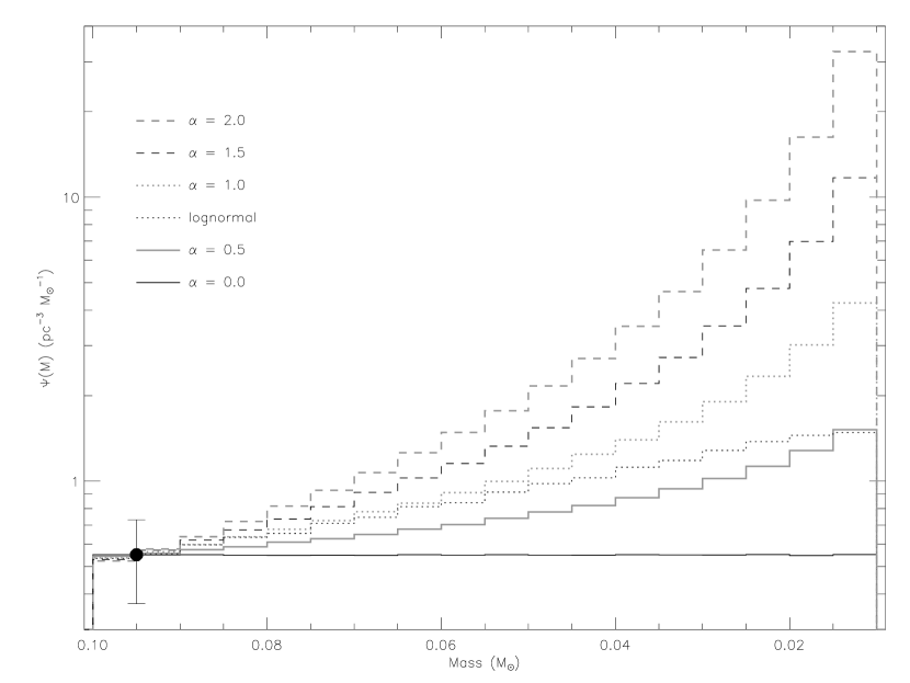
Figure 3: Mass function distributions ($\Psi({\rm M})$; number density per Solar mass) derived from the Monte Carlo simulations, for baseline parameters ($P(t)$ = constant, $0.1<t<10$ Gyr, and $0.01<{\rm M}<0.1$ M_☉). Distributions are sampled every 0.005 M_☉. These results agree with the analytic forms to 5% or better, even for lower minimum mass limits. The normalization constant for the simulations, 0.55$\pm$0.18 pc^-3 M${}_{\sun}^{-1}$ at 0.095 M_☉, based on the low-mass star MFs of Reid et al. (1999) and Chabrier (2001), is indicated by the solid circle.

Figure 3 shows the resulting MF distributions for simulations with baseline parameters: Baraffe evolutionary models, $P(t)$ = constant, $0.01\leq{\rm M}\leq 0.1$ M_☉, and $0.01\leq t\leq 10$ Gyr. These distributions are consistent with their analytic forms to better than 3% over most of the mass range examined, with somewhat larger scatter (not exceeding 10%) in the lowest mass bins for the steepest power law distributions. These accuracies are identical for simulations using lower cutoff masses. Therefore, numerical uncertainties are negligible in comparison to, e.g., observational uncertainties (Paper II) and differences between the evolutionary models ($\S$4.2.1).

3 Results

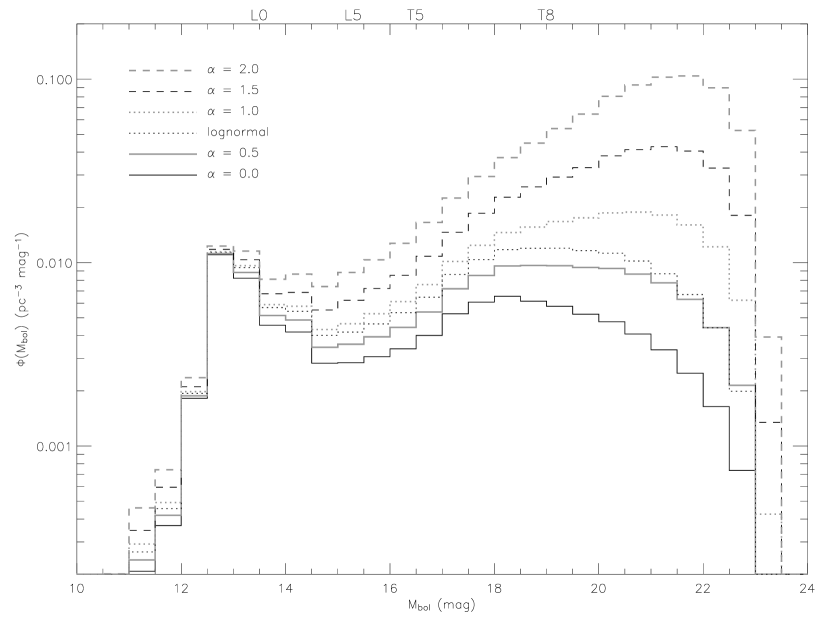
Figure 4: Derived luminosity functions ($\Phi(M_{bol})$; number density per magnitude) for the baseline MF simulations (Baraffe et al. (2003) models, $0.01\leq$ M $\leq 0.1$ M_☉, $0.01\leq t\leq 10$ Gyr, and constant birthrate). Distributions are sampled every 0.5 mag. The approximate location of spectral types L0, L5, T5, and T8 are indicated, based on empirical $M_{bol}$ determinations from Golimowski et al. (2004).

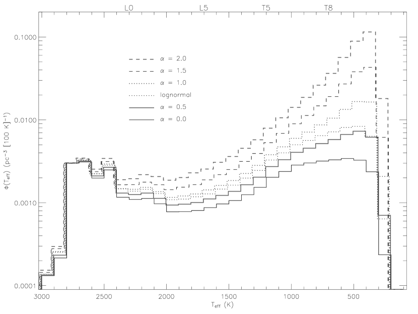
Figure 5: Derived T_eff distributions ($\Phi({\rm T}_{eff})$; number density per 100 K) for the baseline MF simulations. Distributions are sampled every 100 K, and are slightly offset horizontally for clarity. The approximate location of spectral types L0, L5, T5, and T8 are indicated, based on empirical T_eff determinations from Golimowski et al. (2004).

A total of 32 Monte Carlo simulations were run to examine the various input parameters described above. Resulting observable distributions for the baseline simulations are given in Tables 3 and 4 and diagrammed in Figures 4 and 5.

3.1 The Luminosity Function

Figure 4 diagrams the derived LFs, $\Phi(M_{bol})$, for baseline parameters and for each of the MFs examined. Also labelled in this plot (and subsequent figures) are the approximate $M_{bol}$s for spectral types (SpT) L0, L5, T5, and T8, based on empirical measurements by Golimowski et al. (2004). At bright magnitudes, there is a peak at $M_{bol}\sim 13$ (SpT $\lesssim$ L0) which is less pronounced for the steeper MFs but yields the same density of objects (0.01 pc^-3 mag^-1) for all MFs. This peak is almost entirely comprised of low mass stars (0.08 $<$ M $<$ 0.1 M_☉), and the fixed density reflects the adopted normalization. The drop off in $\Phi(M_{bol})$ toward brighter luminosities is an artifact of the upper mass limit (0.1 M_☉) of the simulations. At $M_{bol}\sim 15$ (SpT $\sim$ L5) there is a local minimum in $\Phi(M_{bol})$, a feature that has also been seen in the simulations of Chabrier (2003) and Allen et al. (2004, their “Trough B”). The origin of this trough may be seen in the divergence of the evolutionary tracks in Figure 2 around T${}_{eff}\sim 1800$ K (corresponding to $M_{bol}\sim 15$). At late ages, this temperature straddles the HBMM, and hence most brown dwarfs have cooled to lower temperatures and fainter luminosities. Sources older than 1 Gyr tend to dominate the overall population for a flat birthrate (see $\S$ 4.1); hence, the narrow range of masses sampling these luminosities at late ages implies fewer sources overall. Note that shallower power laws produce a more pronounced trough. Toward fainter magnitudes, $\Phi(M_{bol})$ rises, more significantly for steeper power laws due to the greater proportion of low mass (and hence intrinsically fainter for a given age) brown dwarfs. Each distribution exhibits a broad peak at these faint magnitudes, with the location of the maximum depending on the steepness of the MF: $M_{bol}\sim 18$ for $\alpha$ = 0 and $M_{bol}\sim 22$ for $\alpha$ = 2. Indeed, beyond $M_{bol}\sim 18$ (SpT $\sim$ T7), there is a substantial increase in the contrast between the various MFs, with up to 25 times more brown dwarfs between $\alpha$ = 2 and 0 at M${}_{bol}\sim 21$. The lognormal $\Phi(M_{bol})$ lies between those of the $\alpha$ = 0.5 and 1.0 MFs, and is generally flat between $18\lesssim M_{bol}\lesssim 21$. Below $M_{bol}\sim 22$, there is a steep drop off in all of the $\Phi(M_{bol})$ distributions due to both the adopted lower mass limit (0.01 M_☉ for the simulations diagrammed in Figure 4) and the adopted maximum age (10 Gyr). A lower minimum mass and/or and an older population would result in a turnover in the LF at fainter magnitudes.

3.2 The T_eff Distribution

Figure 5 compares the $\Phi(T_{eff})$ distributions for the same simulations. The bright magnitude peak seen in the $\Phi(M_{bol})$ distribution is evident at $T_{eff}\sim 2500-2700$ K, although it likely underestimates the actual number of stars/brown dwarfs at these higher temperatures because of the 0.1 M_☉ upper mass cutoff. The trough in $\Phi(M_{bol})$ is also seen here, albeit somewhat less pronounced, around 1800–2000 K (SpT $\sim$ L3-L5), again due to the rapid cooling of brown dwarfs at these temperatures. At lower $T_{eff}$s, all of the distributions rise, with the steeper power laws yielding at least an order of magnitude more cold brown dwarfs (T${}_{eff}\sim 500$ K) than warm ones (T${}_{eff}\sim 2000$ K). At 1000 K (SpT $\sim$ T6), there is a factor of 8 difference between $\alpha$ = 0 and 2, and a factor of 30 difference at 500 K. The resulting densities of cold brown dwarfs are fairly high, predicting roughly 25 brown dwarfs with 400 $\lesssim$ T_eff $\lesssim$ 800 K within 5 pc of the Sun for $\alpha$ = 1. This is somewhat less than half the number of main sequence stars in an equivalent volume (Reid, Gizis, & Hawley, 2002). Below 300 K, there is a sharp turnover in $\Phi({\rm T}_{eff})$ similar to that seen in $\Phi(M_{bol})$ for $M_{bol}\lesssim 22$.

4 Analysis

4.1 Composition of $\Phi(M_{bol})$ and $\Phi({\rm T}_{eff})$

It is instructive to break down the luminosity and T_eff distributions by mass and age in order to examine in detail the origins of the various features seen. Figure 6 shows $\Phi({\rm T}_{eff})$ for the $\alpha$ = 0.5 simulation for which a low mass cutoff of 0.001 M_☉ was used (see $\S$ 4.2.3). This distribution is broken down into groupings of low mass stars (0.075 $<$ M $<$ 0.1 M_☉), Deuterium-burning brown dwarfs (0.012 $<$ M $<$ 0.075 M_☉), and non-fusing brown dwarfs (0.001 $<$ M $<$ 0.012 M_☉). It is clear that the high temperature peak in the LF is indeed dominated by main sequence low-mass stars down to 1900–2000 K (SpT $\sim$ L3), with a smaller contribution of predominantly young Deuterium-burning brown dwarfs. At cooler temperatures, Deuterium-burning brown dwarfs are the dominant population down to T${}_{eff}\sim 500$ K, encompassing all of the currently known field brown dwarfs. Non-fusing brown dwarfs only make a significant contribution below this temperature. This segregation of masses in the $\Phi({\rm T}_{eff})$ distribution is seen for all of the MFs examined.

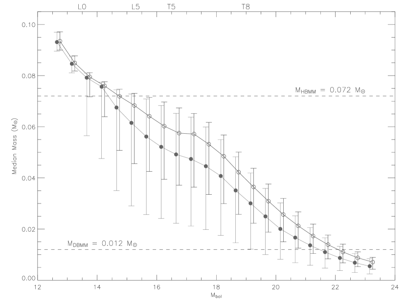
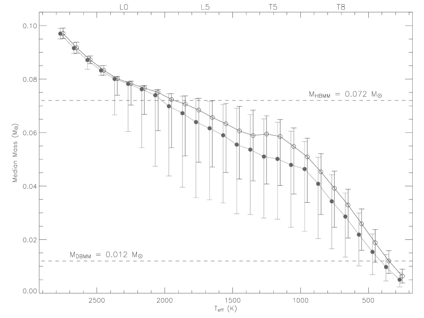
Figure 7: Median mass versus $M_{bol}$ (left) and T_eff (right) for baseline power-law MF simulations with $\alpha$ = 0.5 (black, open circles) and 1.5 (grey, filled circles). The uncertainty of the typical mass in each bin is indicated as the range of masses sampled by 63% of the population about the median, consistent with Gaussian $\pm$1$\sigma$ uncertainties. Data points are slightly offset horizontally for the $\alpha$ = 1.5 case for clarity. The Hydrogen and Deuterium burning mass limits (0.072 and 0.012 M_☉, respectively) for the Baraffe models are delineated by dashed lines.

An alternate way to examine the mass composition of $\Phi(M_{bol})$ and $\Phi({\rm T}_{eff})$ is by computing the median mass per luminosity or T_eff bin, as diagrammed in Figure 7 for simulations with M_min = 0.001 M_☉ and $\alpha$ = 0.5 and 1.5. The most likely range of masses in each bin was chosen to comprise 63% of all objects about the median value, equivalent to $\pm$1$\sigma$ in a Gaussian distribution. Three trends are immediately discernable; first, the median mass decreases toward lower luminosities and cooler temperatures, consistent with the fact that lower-mass brown dwarfs start off cooler, and therefore remain cooler, than their higher-mass counterparts at any given age. Second, as the median mass relations cross the HBMM, they diverge for different MFs, with the steeper distributions exhibiting lower median masses at a given luminosity or temperature. This is simply due to the larger number of lower-mass brown dwarfs in the steeper MFs contributing to each of the luminosity and temperature bins. Finally, there is a wide range of masses that comprise each luminosity and temperature bin, a range that increases for steeper MFs with the inclusion of more low-mass sources. In one sense, these substantial mass “uncertainties” highlights the motivation for the simulations — the non-unique nature of the field substellar M-L relation — and demonstrates the substantial uncertainty in assigning masses to field objects without age information.

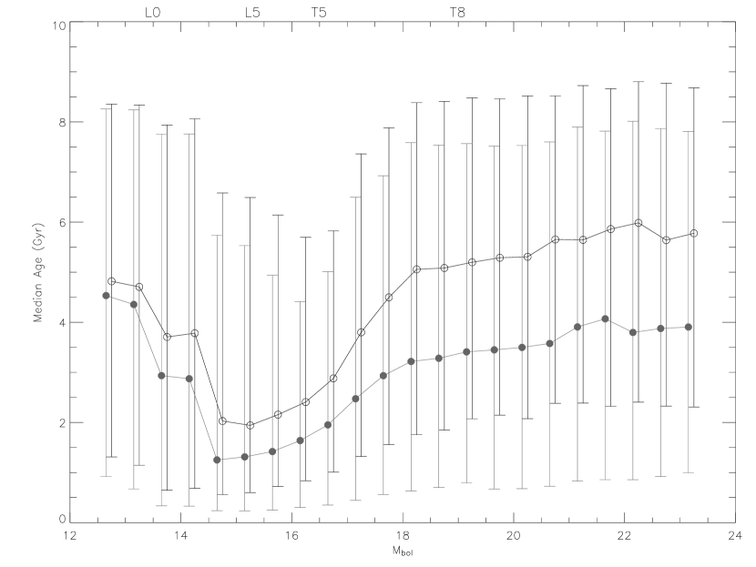
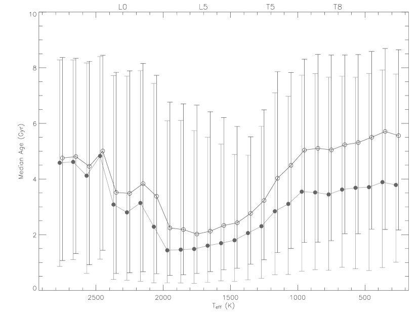
Figure 8: Median age versus $M_{bol}$ (left) and T_eff (right); symbols are those of Figure 8. Scatter in the ages for each bin are indicated and were calculated similarly to the mass uncertainties in Figure 8. Data points are slightly offset horizontally for the $\alpha$ = 1.5 case for clarity.

Figure 8 plots the median age as a function of luminosity and T_eff for the same MF simulations; the indicated typical range of ages was computed as above. In this case, the spread in ages in each bin is substantial; it is not possible to assign a statistical age with uncertainty better than a few Gyr based on luminosity and T_eff alone. However, there are some subtle trends in these relations that may have statistical merit. There is a notable drop in the median age at the same locations as the troughs in the $\Phi(M_{bol})$ and $\Phi({\rm T}_{eff})$ distributions, around 1500 $\lesssim$ T_eff $\lesssim$ 2000 K. These features are related, as the higher luminosities and hence more rapid evolution of brown dwarfs at these temperatures implies both fewer objects present at any given time and very few brown dwarfs remaining or reaching these temperatures at later ages. At earlier times, this temperature region encompasses a much broader range of masses and hence a larger percentage of the young population. Allen et al. (2004) note a similar age bias amongst L dwarfs in their simulations. One consequence of this feature is that L dwarfs in the field should be younger on average than T dwarfs. There is some empirical evidence of this form tangential velocity measurements (Vrba et al., 2004) and the mass-age-activity trends of late-type M and L dwarfs (Gizis et al., 2000). However, it is important to stress that the range of ages sampled at these temperatures is still very large, and individual age determinations cannot be precisely determined. The apparent decrease in median age for steeper power-law MFs is again due to the greater contribution of lower-mass brown dwarfs, which appear in the higher temperature and luminosity bins when they are younger and less evolved.

4.2 Variations in $\Phi$ Distributions from Various Factors

The observable distributions presented above are based primarily on the baseline parameters of a flat birth rate, $0.01\leq{\rm M}\leq 0.1$ M_☉, $0.01\leq t\leq 10$ Gyr, and the Baraffe et al. (2003) evolutionary models. The trends identified in these distributions indicate methods of constraining the substellar MF by comparison to empirical data; however, they may be confused by other details such as the choice of evolutionary model, the form of the birth rate, the age range of field brown dwarfs, and the minimum formation mass. Quantifying the influence of these parameters on the shape and scale of the observable distributions provides a measure of the systematic uncertainty in the derived MF when comparing to empirical data.

4.2.1 Variations due to Choice of Evolutionary Model

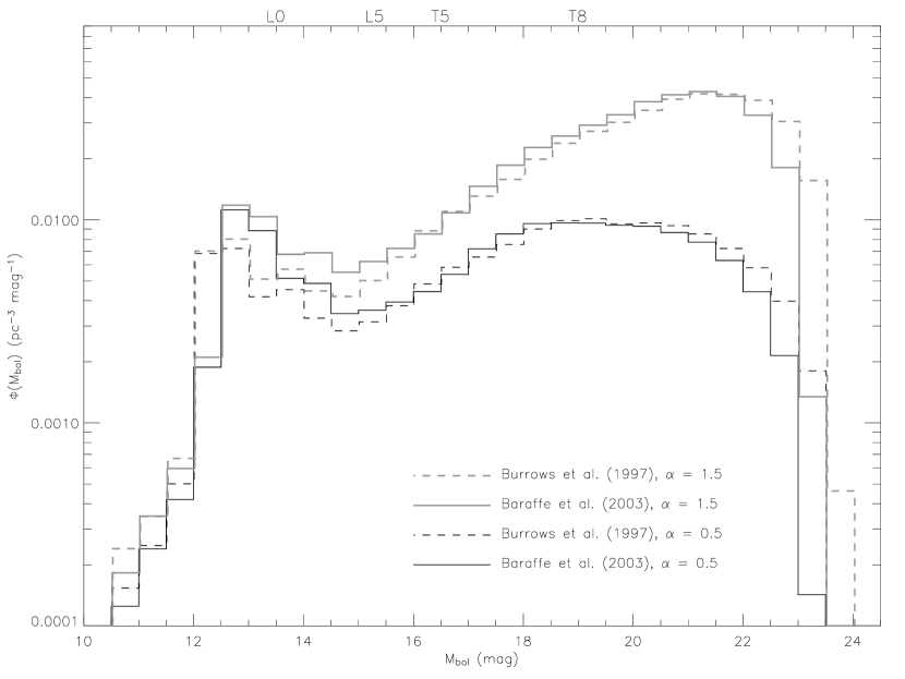
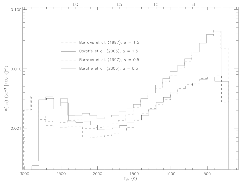
Figure 9: Comparison of $\Phi(M_{bol})$ (left) and $\Phi({\rm T}_{eff})$ (right) for $\alpha$ = 0.5 (black lines) and 1.5 (grey lines) baseline simulations based on the Burrows et al. (1997, dashed lines) and Baraffe et al. (2003, solid lines) evolutionary models. Distributions are slightly offset horizontally for clarity.

Figure 9 compares $\Phi(M_{bol})$ and $\Phi({\rm T}_{eff})$ between the Burrows et al. (1997) and Baraffe et al. (2003) models for the $\alpha$ = 0.5 and 1.5 power-law MFs. Some of the variations in the tracks seen in Figure 2, particularly at the stellar/substellar boundary, are reflected in the resulting observable distributions. Most notably, the bright peak at $M_{bol}\sim 13$ (T${}_{eff}\sim 2500$ K) is far less pronounced in the Burrows et al. (1997) model simulations. Low mass stars are instead piled up at slightly brighter luminosities ($M_{bol}\sim 12.5$) and hotter temperatures (T${}_{eff}\sim 2800$ K). Furthermore, the Burrows et al. (1997) models predict fewer objects overall at brighter magnitudes ($M_{bol}\lesssim 15$) and hotter temperatures (T${}_{eff}\gtrsim 1500$ K), and more objects at fainter magnitudes ($M_{bol}\gtrsim 22$) and colder temperatures (T${}_{eff}\lesssim 400$ K) than the Baraffe et al. (2003) models. In the T dwarf regime, however, the two sets of models are in fairly good agreement for all of the MFs examined. Therefore, the choice of evolutionary model does not appear to affect the interpretation of the T dwarf field LF, but can be an important source of systematic uncertainty when examining the LF of hotter (L- and M-type) brown dwarfs.

4.2.2 Variations due to Differing Birth Rates

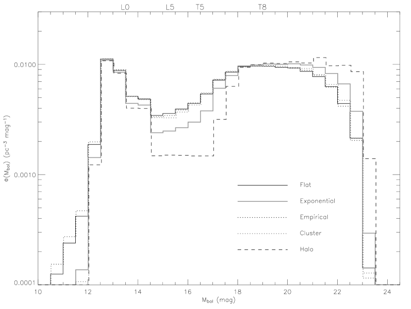
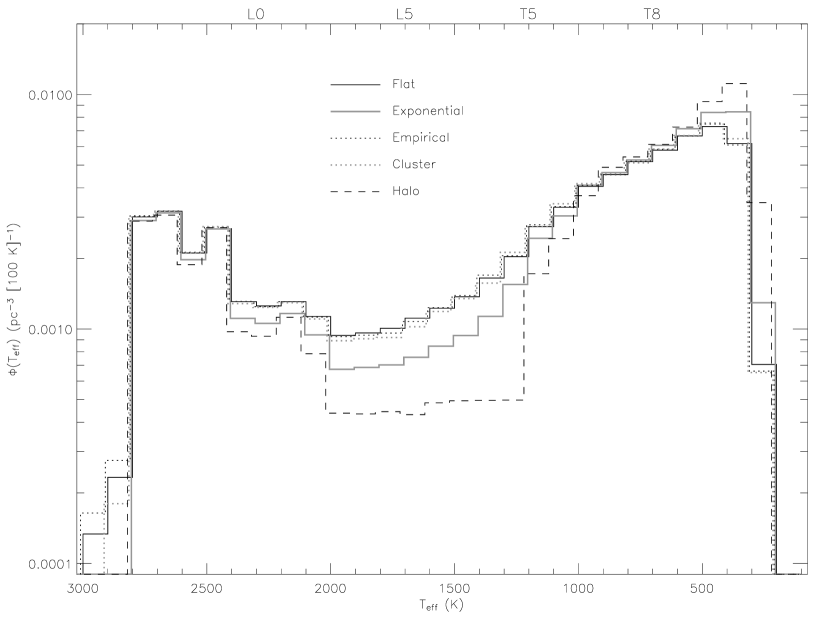
Figure 10: Comparison of $\Phi(M_{bol})$ (left) and $\Phi({\rm T}_{eff})$ (right) for $\alpha$ = 0.5 baseline simulations for the five birth rates explored in this study. Distributions for each birthrate are slightly offset for clarity. The constant, empirical, and cluster birth rates show nearly identical distributions, while the exponential and halo distributions show significant variations in the $M_{bol}\sim 15-17$ (T${}_{eff}\sim 1200-2000$ K; SpT T5-L3) trough and at faint luminosities/cold temperatures. Distributions are slightly offset horizontally for clarity.

Figure 10 compares $\Phi(M_{bol})$ and $\Phi({\rm T}_{eff})$ for the five birthrates for an $\alpha$ = 0.5 baseline simulation. For both distributions, there is effectively no difference between the constant, empirical, and stochastic birth rates, the more realistic realizations for the Galactic field population. This result is consistent with the findings of Allen et al. (2004), who discern minimal variations in derived LFs between birth rates that are constant, based on field star ages (Soderblom, Duncan, & Johnson, 1991), and based on star formation rates as a function of redshift (Pascual et al., 2001). Therefore, the underlying birth rate generally has a negligible effect on the determination of the field MF.

The more extreme exponential and halo birth rates, however, do modulate the observable distributions, with a far more pronounced dip at $M_{bol}\sim 15-17$ (T${}_{eff}\sim 1200-2000$ K; SpT $\sim$ T5-L3) and more fainter/cooler brown dwarfs. Both of these effects are due to the larger proportion of older, and therefore more evolved and fainter, brown dwarfs produced by these birth rates. The differences are most pronounced for the halo age distribution, which predicts a substantial deficiency of T${}_{eff}\approx 1200-2000$ K brown dwarfs, comprised primarily of mid- and late-type L and early T dwarfs. Note that this deficiency is likely to be more pronounced in a real halo population, as the reduced metallicity typical for halo dwarfs (Gizis, 1997) imply more transparent atmospheres, enhanced luminosities, and hence more rapid cooling (Burrows et al., 2001).

It is interesting to note that all of the distributions are generally consistent between $18\lesssim M_{bol}\lesssim 21$ (500 $\lesssim$ T${}_{eff}\lesssim 1000$ K), which encompasses mid- and late-type T dwarfs. These consistencies suggest that while the field T dwarf population may be highly sensitive to the underlying MF ($\S$ 3.1), it is generally insensitive to the birth rate. In contrast, the L dwarf field population is somewhat less sensitive to the MF but may be an excellent probe of extreme Galactic birth rates. These trends are also seen in the steeper MFs.

4.2.3 Variations due to Differing Age Limits

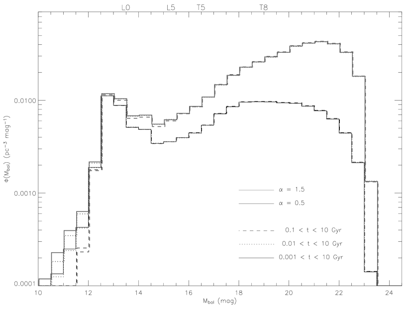
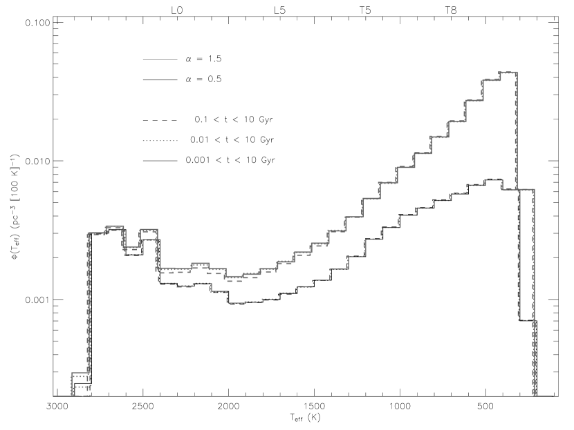
Figure 11: Comparison of $\Phi(M_{bol})$ (left) and $\Phi({\rm T}_{eff})$ (right) for $\alpha$ = 0.5 (black lines) and 1.5 (grey lines) baseline simulations for four minimum age limits, $t$ = 0.001 (solid lines), 0.01 (dotted lines), 0.1 (dashed lines), and 1 (dot-dashed lines) Gyr. Distributions are slightly offset horizontally for clarity.

Figure 11 compares $\Phi(M_{bol})$ and $\Phi({\rm T}_{eff})$ for minimum ages of 1 to 100 Myr for the $\alpha$ = 0.5 and 1.5 MFs. No significant differences are seen between these LFs, primarily because very young ($t<100$ Myr) brown dwarfs contribute minimally ($\sim$1% for a flat birthrate) to the 10 Gyr field LF over the mass range examined. Hence, the minimum age of the substellar field population only influences the observed LF if it is of order 1 Gyr or later, as seen with the halo birthrate discussed above.

4.2.4 Variations due to Differing Minimum Mass Cutoffs

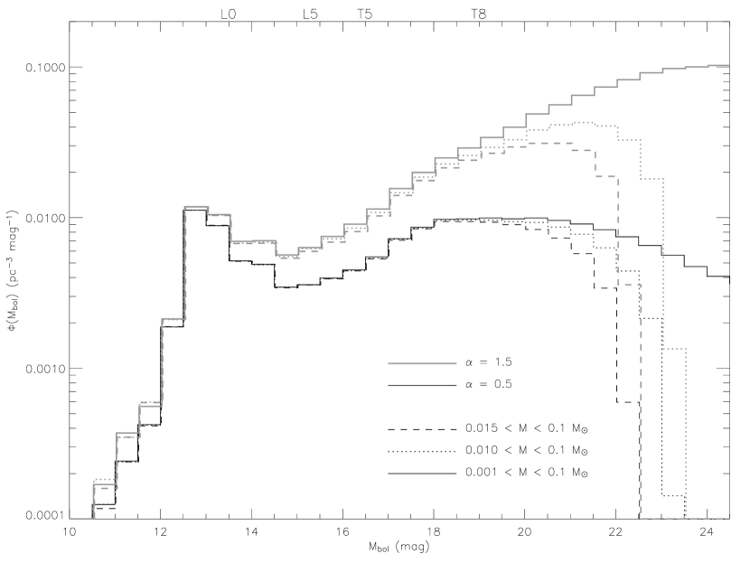
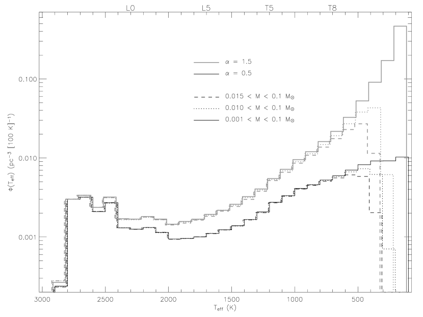
Figure 12: Comparison of $\Phi(M_{bol})$ (left) and $\Phi({\rm T}_{eff})$ (right) for $\alpha$ = 0.5 (black lines) and 1.5 (grey lines) baseline simulations for three minimum formation masses: M_min = 0.001, 0.010, and 0.015 M_☉. Distributions are slightly offset horizontally for clarity.

One of the key parameters for low-mass star formation theories is the minimum formation mass, which depends not only on the thermodynamical conditions of the initial gas reservoir (through the Jean’s mass, Jeans 1902), but also on the efficiency and history of accretion early in the formation process. Figure 12 compares $\Phi(M_{bol})$ and $\Phi({\rm T}_{eff})$ for minimum formation masses M_min = 0.001, 0.010, and 0.015 M_☉ and the $\alpha$ = 0.5 and 1.5 MFs. As expected, reducing M_min results in many more intrinsically faint objects, and the low-temperature turnover in $\Phi({\rm T}_{eff})$ (Figure 5) is essentially absent for M_min = 0.001 M_☉. However, the differences between these distributions are negligible for $M_{bol}\lesssim 20$ and T${}_{eff}\gtrsim 500$ K for both power-law MFs. This is consistent with the mass breakdown of $\Phi({\rm T}_{eff})$ in Figure 6, which shows that the lowest mass brown dwarfs contribute significantly only to the lowest temperature/luminosity bins. Thus, the signature of a minimum brown dwarf formation mass, unless it is larger than 0.015 M_☉, cannot be detected in the currently known sample of field brown dwarfs, which extend only to T${}_{eff}\sim 700$ K (Golimowski et al., 2004; Vrba et al., 2004). Determining M_min from field measurements will require the discovery of substantially cooler brown dwarfs.

4.3 The Influence of Multiplicity

Any observed sample of stars or brown dwarfs may include some percentage of unresolved multiple systems. Indeed, stellar multiples are more frequent amongst Solar-mass stars than single systems (Abt & Levy, 1976; Duquennoy & Mayor, 1991, $\sim 60$%), and this frequency may be even higher during the early T-Tauri phase (Ghez, Neugebauer, & Mattews, 1993). Recent high-resolution imaging studies of low-mass stars and brown dwarfs have shown that a small fraction of these systems ($\sim$10–20%) are closely-separated ($a\lesssim 15$ AU) binaries (Koerner et al., 1999; Reid et al., 2001; Close et al., 2002; Bouy et al., 2003; Burgasser et al., 2003b; Gizis et al., 2003), and at least one substellar spectroscopic binary is also known (Basri & Martín, 1999a). All of these systems are unresolved in wide-field imaging surveys such as 2MASS and SDSS; hence, brown dwarf samples drawn from those surveys tend to measure the systemic LF, $\Phi_{sys}$, rather than the distribution of individuals, $\Phi_{ind}$. The latter is a more appropriate constraint for star formation theory or the Galactic mass budget.

Unresolved multiple systems induce two effects on the LF: (1) an increase in the number of individual sources in the sample; and (2) an increase in the effective volume sampled for each of the individual components of a multiple system, as their unresolved combined light allows them to be detected to greater distances. To examine these effects, a second series of Monte Carlo simulations were performed, building from the $\Phi({\rm T}_{eff})$ distributions from the MF simulations. It was assumed that the sample under investigation is a magnitude-limited one for which T_effs can be measured (e.g., through spectral typing or color), the typical scenario for samples large enough to measure the mass function. Furthermore, only coeval binary systems were considered, and it was assumed that the binary fraction ($f_{bin}$; higher order systems are ignored) and mass ratio ($q\equiv{\rm M}_{2}/{\rm M}_{1}$) distribution ($P(q)$) are fixed and independent of mass, and can therefore be treated separately from $\Psi({\rm M})$ and $P(t)$. Finally, it was assumed that the primary of each system has the same temperature (T${}^{(1)}_{eff}$) as the observed systemic T_eff, as would be the case if the unresolved spectrum (and hence spectral type) is dominated by the brighter component.

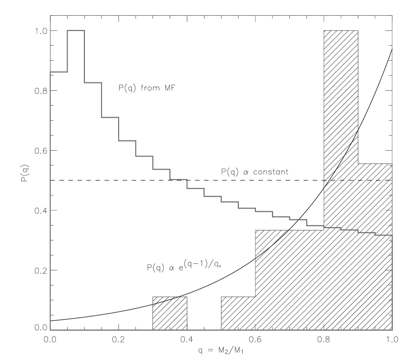
Figure 13: $P(q)$ distributions employed to examine the effects of unresolved multiplicity: (dashed line) $P(q)\propto$ constant; (black line) $P(q)\propto{\rm e}^{(q-1)/q_{c}}$; (grey histogram line) $P(q)$ from random pairing of primaries and secondaries drawn from an $\alpha$ = 0.5 MF with M_min = 0.001 M_☉. All distributions are arbitrarily normalized. The exponential distribution (with $q_{c}=0.26$) was chosen to fit an empirical mass ratio distribution (hatched histogram) constructed from 22 L and T dwarf binaries from Reid et al. (2001), Bouy et al. (2003), Burgasser et al. (2003b), and Gizis et al. (2003).

An analytic approximation to this problem, appropriate for the overall space density of a population, is given in the Appendix. For the simulations, the effect of multiplicity on the observed $\Phi({\rm T}_{eff})\equiv{\Phi}_{sys}({\rm T}_{eff})$ was considered by determining the correction factor ${\Phi}_{ind}({\rm T}_{eff})/{\Phi}_{sys}({\rm T}_{eff})$. First, ${\Phi}_{sys}({\rm T}_{eff})$ was scaled by $(1-f_{bin})$ to give the number density of single objects. The remaining $f_{bin}$ fraction of binary systems were modelled using $N$ = 10⁶ test sources per T_eff bin. Mass ratios for the binaries were assigned from three choices of $P(q)$, listed in Table 1 and diagrammed in Figure 13, where $q$ was allowed to vary from 0.001 to 1. The first (“flat”) distribution is generally consistent with results from closely-separated (spectroscopic) stellar binary studies (e.g., Mazeh et al. 1992, 2003). The second (“exponential”) distribution assumes a greater percentage of equal-mass systems, a form consistent with recent studies of low-mass star and brown dwarf binaries (Reid et al., 2001; Gizis et al., 2003; Goldberg, Mazeh, & Latham, 2003). A value of $q_{c}$ = 0.26 was derived from a fit to the apparent $q$ distribution of known L and T dwarf binaries (Reid et al., 2001; Bouy et al., 2003; Burgasser et al., 2003b; Gizis et al., 2003, Figure 13). Note that this empirical distribution has not been corrected for selection effects (e.g., incompleteness for low-$q$ systems), and is therefore purely an exploratory one. The third distribution assumes both primaries and secondaries are drawn from the same underlying MF, an interpretation put forth by Duquennoy & Mayor (1991) to explain the mass ratio distribution of G and K stars (see also Kroupa & Burkert 2001). The distribution shown in Figure 13, which peaks at lower mass ratios, was generated from Monte Carlo simulations of 10⁶ primaries and 10⁶ secondaries, both drawn from an $\alpha$ = 0.5 power-law mass function with M_min = 0.001 M_☉, and random pairing ($q$ is fixed to be no greater than unity).

For each binary simulation, effective temperatures for the secondary components of the binaries, T${}^{(2)}_{eff}$, were determined as:

$$\frac{{\rm T}^{(2)}_{eff}}{{\rm T}^{(1)}_{eff}}\approx\left(\frac{{\rm L}^{(2)}}{{\rm L}^{(1)}}\right)^{1/4}\approx q^{0.66},$$ (13)

where it is assumed that the primary and secondary radii are equal (true to within 10-15% for ages greater than 1 Gyr) and L $\propto$ M^2.64 (Burrows et al., 2001). Equation 13 matches theoretical evolutionary models fairly well but can overestimate T${}^{(2)}_{eff}$ by 10-20% for systems that staddle the H- or D-burning limits. It is, however, a useful analytical approximation. The $N_{sec}=f_{bin}N$ secondaries were then binned by their T_eff, and the space density of both primaries and secondaries added to the single star $\Phi({\rm T}_{eff})$ distribution after scaling by the factor:

$$\hat{\epsilon}({\rm T}_{eff})\equiv\frac{1}{N_{sec}}\sum_{i}^{n({\rm T}_{i}={\rm T}_{eff})}(1+q_{i}^{2.64})^{-3/2},$$ (14)

where the sum is over the $n$ simulated primaries or secondaries for which T_i = T_eff (after binning). The factor $(1+q_{i}^{2.64})^{-3/2}\equiv{\epsilon}_{i}$ compensates for the increased volume sampled by the combined light of the binary system (see Appendix, Eqn. A3). Thus, for each T_eff bin $k$, the temperature distribution of individual sources is

$$\begin{array}[]{rcl}\Phi_{ind}({\rm T}_{k})&=&(1-f_{bin})\Phi_{sys}({\rm T}_{k})\\ &+&f_{bin}{\Phi}_{sys}({\rm T}_{k})\hat{\epsilon}({\rm T}_{k})\\ &+&f_{bin}{\sum_{j}\Phi_{sys}({\rm T}_{j}^{(1)}{\mid}{\rm T}_{j}^{(2)}={\rm T}_{k})\hat{\epsilon}({\rm T}_{j}^{(2)})}\end{array}$$ (15)

where the final term incorporates secondaries for which T${}_{j}^{(2)}$=T_k, but normalizes to the systemic space density corresponding to the temperature of the primary.

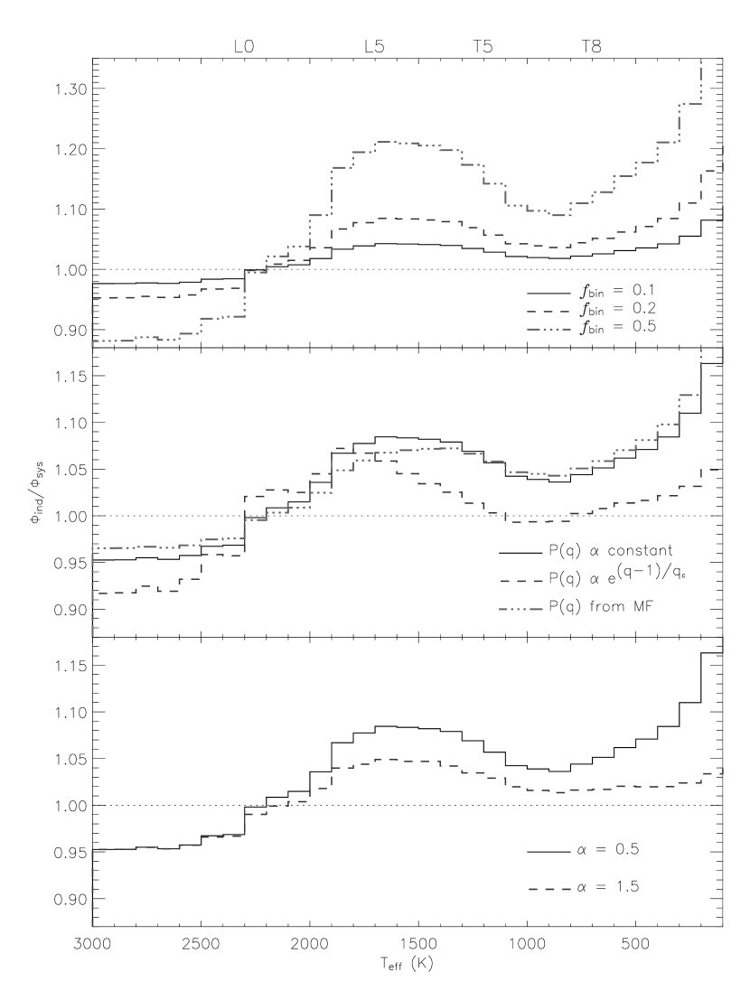
Figure 14: Multiplicity corrections $\Phi_{ind}/{\Phi}_{sys}$ for a magnitude-limited survey that includes unresolved binary systems. Top panel: Variations as a function of binary fraction, $f_{bin}$ = 0.1, 0.2, and 0.5, assuming a flat mass ratio distribution ($P(q)$ = constant) and $\alpha$ = 0.5. Center panel: Variation between the three $P(q)$ distributions employed (Table 1), assuming $f_{bin}$ = 0.2 and $\alpha$ = 0.5. Bottom panel: Variations between two power-law MFs, $\alpha$ = 0.5 and 1.5, assuming $P(q)$ = constant and $f_{bin}$ = 0.5.

Figure 14 plots $\Phi_{ind}/\Phi_{sys}$ as a function of T_eff for various assumptions of $f_{bin}$, $P(q)$, and $\alpha$. All of distributions show significant structure, with correction values less than unity for T${}_{eff}\lesssim$ 2300 K (SpT $\sim$ L0), large correction values for T_eff $\sim$ 1300–1700 K (SpT $\sim$ T0-L5), a dip around T_eff $\sim$ 900 K (SpT $\sim$ T7), and a rapid rise toward the coolest temperatures. Most of this structure can be attributed to a trickle-down effect amongst the binary secondaries. The low values of $\Phi_{ind}/\Phi_{sys}$ for hotter dwarfs is due to the lack of secondaries from systems with primaries having M $>$ 0.1 M_☉ in these simulations; hence, only equal-mass/equal-magnitude binaries contribute. As discussed in the Appendix, a mass-ratio distribution skewed toward $q=1$ causes the increased effective volumes of these systems to be a larger effect than the addition of secondaries into the sample. This feature, then, is an artifact of our simulation upper mass limit. The peak at T${}_{eff}\sim$ 1300–1700 K is enhanced by both the decline of the underlying LF at these temperatures and the addition of low- and moderate-$q$ secondaries associated with primaries from the 2500–2700 K $\Phi({\rm T}_{eff})$ peak. The valley in $\Phi_{ind}/\Phi_{sys}$ at cooler temperatures is the result of the opposite trend: a rise in the underlying LF at these temperatures coincident with a paucity of hotter host primaries hosting low- and moderate-$q$ secondaries. At the coolest temperatures, very low-mass secondaries associated with primaries across the LF contribute to $\Phi_{ind}$, and a large correction factor is needed to account for these systems. Note that mass ratio distributions skewed toward higher mass ratios (e.g., the exponential $P(q)$) result in a smaller correction factor beyond T_eff $\sim$ 1800 K, due to the paucity of low-mass secondaries contributing to the lower temperature bins. A similar trend is seen for steeper MFs, but in this case is due to the steeper rise of the underlying LF at lower temperatures.

The morphology of $\Phi_{ind}/\Phi_{sys}$ implies that unresolved multiplicity tends to enhance key features in the LF, resulting in a larger contrast between L and T dwarf numbers in the observed $\Phi_{sys}$. On the other hand, the very coolest and faintest brown dwarfs in an observed sample are largely hidden as low-$q$ secondaries, resulting in an artificial flattening of the LF. It is important to note, however, that these variations are generally small. For binary fractions typical for brown dwarf systems, ${\mid}1-\Phi_{ind}/\Phi_{sys}{\mid}<10$% for T${}_{eff}\gtrsim 300$ K, similar to the systematic uncertainties from the evolutionary models and far more accurate than current LF measurements of late-type field dwarfs (e.g., Cruz et al. 2003). Even binary fractions as high as 50% cause only a 20% shift in the LF in the late L dwarf regime. Hence, the influence of unresolved multiplicity will be difficult to discern in the field LF given the current precision of observations; however, as larger field samples are generated, the features described above could provide an independent means of probing the mass ratio distribution of low mass stars and brown dwarfs.

5 Surface Density Predictions

The purpose of the simulations presented here is to place constraints on the substellar MF using LF measurements of field brown dwarfs, an issue that will be pursued in detail in Paper II. The simulations can alternately be used as a predictive tool; specifically, as a means of estimating the number of brown dwarfs detectable in a particular field imaging survey. To illustrate this, surface densities ($\Sigma$) as a function of T_eff for two types of imaging surveys were examined: a shallow near-infrared survey similar to 2MASS, and a deep red-optical survey at high Galactic latitude, similar to the Great Observatories Origins Deep Survey (Giavalisco, 2004) or the Hubble Ultra Deep Field (UDF, Beckwith et al. 2003).

Starting from the $\Phi({\rm T}_{eff})$ distributions with M_min = 0.001 M_☉, surface densities for a shallow survey were computed by assuming that the space density is constant throughout the volume observed, so that

$$\Sigma_{sh}({\rm T}_{eff})=\frac{1}{3}(\frac{\pi}{180})^{2}\Phi({\rm T}_{eff})d_{max}^{3}({\rm T}_{eff}).$$ (16)

Here, $d_{max}({\rm T}_{eff})=10^{-0.2(M({\rm T}_{eff})-m_{lim})+1}$ pc is the limiting detection distance for brown dwarfs in the survey to an apparent magnitude limit $m_{lim}$, and $M({\rm T}_{eff})$ is the absolute magnitude/T_eff relation for the imaging filter used. The latter can be determined using either theoretical models or empirical data. For a deep, high Galactic latitude survey, $d_{max}$ can be comparable to the scale height of the Galactic disk ($H_{z}$), so that the vertical distribution of sources must be considered. At a height $z$ above/below the Galactic plane, the space density of stars scales as

$$\Phi(z)={\Phi}_{o}{\rm sech}^{2}(\frac{{\mid}z{\mid}}{2H_{z}})$$ (17)

(Reid & Hawley, 2000), where ${\Phi}_{o}$ is the local space density. The resulting surface density can therefore be written as ${\Sigma}_{deep}={\gamma}{\Sigma}_{sh}$, where

$${\gamma}({\rm T}_{eff})=\frac{3}{d_{max}({\rm T}_{eff})^{3}}\int_{0}^{d_{max}({\rm T}_{eff})}{\rm sech}^{2}(\frac{{\delta}\sin{{\mid}{\beta}{\mid}}}{2H_{z}}){\delta}^{2}{\rm d}{\delta},$$ (18)

is the scale height correction factor for a survey field at Galactic latitude $\beta$. Note that corrections to the radial distribution of sources, which is important for deep surveys extending to several kpc scales close in the Galactic plane, are not considered here.

For the shallow imaging case, $H$-band imaging down to $m_{lim}$ = 16 is considered, similar to the sensitivity limits of 2MASS; while a $z^{\prime}$ field to $m_{lim}$ = 28 (AB magnitudes) at $\beta$ = 54$\fdg$5 is considered for the deep imaging case, appropriate for the Hubble UDF. $M_{H}$ and $M_{z^{\prime}}$ versus T_eff relations for single M6-T8 dwarfs were determined empirically using photometry compiled from Dahn et al. (2002) and Knapp et al. (2004); parallax measurements from Dahn et al. (2002), Tinney, Burgasser, & Kirkpatrick (2003), and Vrba et al. (2004); and T_eff determinations from Golimowski et al. (2004). Linear fits of absolute photometry versus $\log_{10}{{\rm T}_{eff}}$ yield:

$$M_{H}({\rm T}_{eff})=50.27-11.65\log_{10}{{\rm T}_{eff}}~{}~{}({\sigma}=0.13~{}{\rm mags})$$ (19)

for 42 sources with 700 $<$ T_eff $<$ 2900 K, and

$$M_{z^{\prime}}({\rm T}_{eff})=45.60-8.96\log_{10}{{\rm T}_{eff}}~{}~{}~{}({\sigma}=0.20~{}{\rm mags})$$ (20)

for 17 sources with 900 $<$ T_eff $<$ 1750 K. These linear relations are extrapolated over the full T_eff range of our sample.

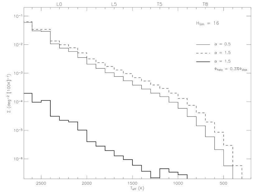
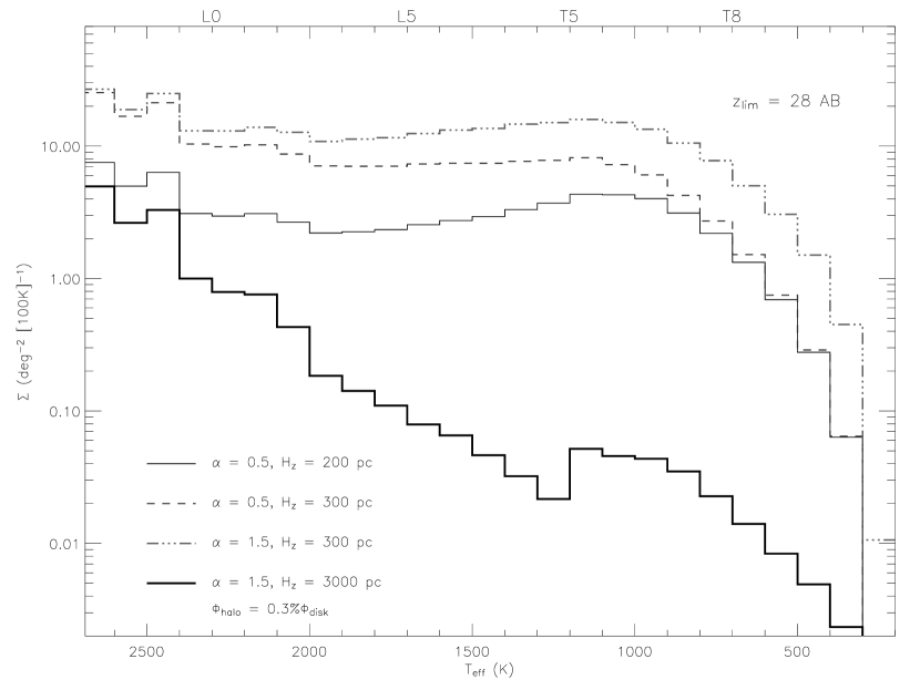
Figure 15: Surface densities ($\Sigma$; in units of deg^-2 [100 K]^-1) as a function of T_eff for a shallow near-infrared survey limited to $H=16$ Vega magnitudes (top) and a deep red optical survey limited to $z^{\prime}$ = 28 AB magnitudes (bottom). For the shallow survey, three cases are shown: $\alpha$ = 0.5 (thin black line) and $\alpha$ = 1.5 (dashed line) disk populations, and an $\alpha$ = 1.5 halo population scaled by 0.3% (thick gray line). For the deep survey, disk scaleheight ($H_{z}$) values of 200 and 300 pc are employed for the disk populations and 3 kpc for the halo population. All models assume a lower mass limit of 0.001 M_☉.

Figure 15 plots ${\Sigma}({\rm T}_{eff})$ for both of the surveys considered. For the shallow case, three populations were examined: “disk” dwarfs with mass functions $\alpha$ = 0.5 and 1.5; and a halo birthrate population with $\alpha$ = 1.5 scaled by a factor of 0.3%, consistent with the relative number of halo to disk stars in the Solar Neighborhood (Reid & Hawley, 2000). In all cases, $\Sigma$ decreases rapidly with T_eff, and the relative densities for the two disk MFs scale with the underlying LF. Halo stars are greatly outnumbered by disk stars, consistent with the adopted normalization, but this contrast increases to $\sim$1% in the T dwarf regime. The low densities in the L and T dwarf regime ($\sim 10^{-5}-10^{-3}$ deg^-2 [100 K]^-1) imply that substantial areas must be imaged to identify a statistically significant number of sources. For the 30,400 deg² T dwarf survey of Burgasser et al. (2003a) examined in Paper II, these simulations (using the stellar density normalization from Reid et al. 1999) predict 22 and 45 disk T dwarfs with 700 $\lesssim$ T_eff $\lesssim$ 1300 for $\alpha$ = 0.5 and 1.5, respectively, independent of color constraints. These values straddle the current number count from this survey, roughly 36 T dwarfs (Burgasser, McElwain, & Kirkpatrick, 2003; Burgasser et al., 2003a, 2004a, in prep; Tinney et al. in prep.).

Surface densities for L and T dwarfs in the deep imaging case are substantially higher ($\sim 2-20$ deg^-2 [100 K]^-1) and approximately constant from 1000 $<$ T_eff $<$ 2500 K. This flattening is caused by the vertical extent of the Galactic disk, which truncates the surface density of warmer sources. For thinner disks ($H_{z}$ = 200 pc), $\Sigma$ is smaller but increases toward cooler T_eff. Hence, both the shape and magnitude of the surface density distribution can provide constraints on the vertical distribution of brown dwarfs for deep imaging surveys. Warmer M- and L-type halo stars and brown dwarfs, for which we assume a larger scale height ($H_{z}$ = 3 kpc), can rival their disk counterparts in surface density despite their lower space density. The coolest brown dwarfs (T_eff $\lesssim$ 800 K) have a surface density distribution similar to the shallow survey case, as these objects are too dim to be detected beyond $H_{z}$. For $H_{z}$ = 300 pc and $\alpha$ = 0.5, these simulations predict 2–3 T dwarfs (500 $\lesssim$ T_eff $\lesssim$ 1300 K) and 3–4 L dwarfs (1300 $\lesssim$ T_eff $\lesssim$ 2300 K; Golimowski et al. 2004) in the 160${\arcmin}^{2}$ UDF $z^{\prime}$ field, sources that could be identified through followup deep imaging and/or spectroscopy.

6 Summary

Monte Carlo simulations of the substellar mass function have been presented, yielding LF and T_eff distributions that can be directly compared to observations. A few salient points are worth reviewing:

• Luminosity and T_eff distributions for relatively simple realizations of the underlying mass function show a complex morphology in the brown dwarf regime, including: (1) a peak at the stellar/substellar limit, (2) a paucity of sources in the L dwarf regime, (3) a rise in number densities for T-type and cooler brown dwarfs, and (4) a low-luminosity peak that depends on the minimum formation mass for brown dwarfs.

• Variations in the stellar birthrate, minimum age, minimum formation mass, and choice of evolutionary model have minimal effect on the LF of T dwarfs, although L dwarf densities can be significantly skewed by any of these. As such, measuring the LF of the local T dwarf population provides the best means of constraining the substellar field MF.

• Determining the minimum formation mass of brown dwarfs in the field will likely require the detection of significant numbers of objects with T_eff $\lesssim$ 500, a temperature regime dominated by very low mass, non-fusing brown dwarfs.

• Field L-type brown dwarfs, which evolve rapidly due to their higher luminosities, may be younger on average than field T dwarfs, a prediction that has some observational support (Gizis et al., 2000; Vrba et al., 2004). For similar reasons, there may be a significant deficit of L-type dwarfs in the Galactic halo ($\tau\geq 9$ Gyr).

• Unresolved multiplicity can enhance features in the observed LF, but these effects are generally small for binary fractions typical of brown dwarfs (10–20%).

• Surface density estimates for the Hubble UDF suggest that a handful of L and T dwarfs will be present in that survey, which can probe the disk scale height of brown dwarfs as well as detect a substantial number of halo low mass stars and brown dwarfs.

The results presented here are qualitatively in agreement with those of Allen et al. (2004), who construct a two-dimensional grid of mass and age distributions to derive L and T_eff distributions for comparison via Bayesian analysis. In particular, many of the features in the LF identified in their simulations also appear here, despite differences in technique. Both studies therefore provide useful tools for constraining the substellar MF in the field.

Paper II in this series will apply the simulations presented here to the local T dwarf LF derived from the 2MASS survey of Burgasser et al. (2003a), improving upon earlier estimates by Burgasser (2001) that were hindered by small number statistics. The simulations can also be used for a wide variety of imaging surveys, both as a predictive tool and as a means of probing the shape and scale of the substellar MF, the age distribution of cool halo dwarfs, the minimum “stellar” formation mass, and the vertical distribution of brown dwarfs in the Galaxy.

Appendix A An Analytic Correction for Space Density Measurements for Unresolved Multiple Systems

Unresolved multiple systems in a magnitude-limited survey can bias LF and space density measurements by hiding unseen members of the sample (underestimating source counts) and skewing photometry-based distance estimates for unresolved systems (overestimating space densities). Since magnitude-limited surveys are commonly used to measure the LF, particularly in the field, an analytic expression for these effects is useful.

Assume that the space density $\phi_{sys}\equiv\int{\Phi(M_{bol})dM_{bol}}$ has been measured for a large, shallow (i.e., ignoring disk scaleheight effects), magnitude-limited, and unresolved sample. Objects in this sample have an intrinsic binary fraction $f_{bin}$ and mass ratio distribution $P(q)$, both of which are independent of mass, luminosity, age, etc. The space density can be represented as a sum over all ($N$) sources in the sample:

$$\phi_{sys}=\sum_{i}^{N}\frac{1}{V_{max,i}}$$ (A1)

(Schmidt, 1968), where

$$V_{max}=\frac{\Omega}{3}d_{max}^{3}=\frac{\Omega}{3}10^{-0.6(M-m_{lim})+3}$$ (A2)

is the maximum volume sampled for a source with intrinsic brightness $M$ to a limiting magnitude $m_{lim}$ over a surface area $\Omega$. Unresolved binaries in this sample with component brightnesses $F^{(1)}$ and $F^{(2)}$, and mass ratios $q\equiv{\rm M}^{(2)}/{\rm M}^{(1)}$, add additional sources to this sum, while also increasing the maximum distances ($d_{max}$) to which they can be detected. For each unresolved binary $i$, the correction to $1/V_{max,i}\propto d_{max,i}^{-3}$ is

$$(1+\frac{F^{(2)}_{i}}{F^{(1)}_{i}})^{-3/2}=(1+q_{i}^{\gamma})^{-3/2}\equiv{\epsilon}_{i}$$ (A3)

(see Eqn. 14), where it is assumed that L $\propto$ M^γ. The space density of individual sources, $\phi_{ind}$, can therefore be expressed in three terms:

$$\phi_{ind}=\sum_{i}^{N_{sin}}\frac{1}{V_{max,i}}+\sum_{i}^{N_{pri}}\frac{{\epsilon}_{i}}{V_{max,i}}+\sum_{i}^{N_{sec}}\frac{{\epsilon}_{i}}{V_{max,i}},$$ (A4)

where $N_{sin}=(1-f_{bin})N$ is the number of single systems and $N_{pri}=N_{sec}=f_{bin}N$ are the number of binary primaries and secondaries, respectively. To the limit of large $N$, variations in individual $V_{max}$ values can be averaged out and the summations replaced by Eqn. A1:

$$\begin{array}[]{rcl}\phi_{ind}&=&(1-f_{bin})\phi_{sys}+2f_{bin}{\Gamma}(q)\phi_{sys}\\ &=&\phi_{sys}(1-f_{bin}(1-2{\Gamma}(q)))\\ \end{array}$$ (A5)

where

$$\Gamma(q)=\int_{0}^{1}{P(q)(1+q^{\gamma})^{-3/2}dq}.$$ (A6)

In the limiting case that all binaries have negligible mass secondaries ($q\rightarrow 0$), $\Gamma(q)\rightarrow 1$, and there is no correction to the distance estimates of the unresolved systems; all of the secondaries are added to the space density. For all binaries in equal-magnitude systems ($P(q)=\delta(q-1)$), $\Gamma(q)=1/\sqrt{2}^{3}$ = 0.354, and $\phi_{ind}=(1-0.293f_{bin})\phi_{sys}$; i.e., $\phi_{ind}<\phi_{sys}$. This is due to the larger $V_{max}$ values for equal-magnitude systems, which overwhelms the increase in $\phi_{ind}$ from the addition of new secondaries. For the $P(q)$ distributions listed in Table 1 and diagrammed in Figure 13, and assuming $\gamma$ = 2.64 (Burrows et al., 2001), $\Gamma(q)>0.5$, so that $\phi_{ind}>\phi_{sys}$. Table 5 lists values for $\phi_{ind}/{\phi_{sys}}$ for various combinations of $f_{bin}$ and $P(q)$. These values are comparable to the simulated corrections diagrammed in Figure 14.

Table 1: Fundamental Distributions for Monte Carlo Simulations.

Distribution	Form	Parameters
(1)	(2)	(3)
$\Psi({\rm M})$	$\propto{\rm M}^{-{\alpha}}$	$\alpha$ = 0.0, 0.5, 1.0, 1.5, 2.0
	$\propto{\rm e}^{-\frac{({\rm\log{M}}-{\rm\log{M_{c}}})^{2}}{2{\sigma}^{2}}}$	${\rm M_{c}}=0.1{\rm M}_{\sun},\sigma=0.627$
$P(t)=b(T_{o}-t)$	$\propto$ constant
	$\propto{\rm e}^{-(T_{o}-t)/{\tau}_{g}}$	To = 10 Gyr, ${\tau}_{g}=5$ Gyr
	empirical
	$\propto\sum_{i=1}^{N_{cl}}{{\rm e}^{-\frac{((T_{o}-t)-t_{o}^{i})^{2}}{2{\tau}_{cl}^{2}}}}$	$N_{cl}=50,{\tau}_{cl}=10$ Myr
	$\propto$ constant $t\leq 1$ Gyr
$P(Z)$	$\propto$ constant	$Z=Z_{\sun}$
$P(q)$	$\propto$ constant
	$\propto{\rm e}^{(q-1)/q_{c}}$	$q_{c}=0.26$
	from MF	$\alpha=0.5$

Table 2: $\Psi({\rm M})$ for Baseline Simulations.

Mass (M☉)	$\alpha$ = 0.0	$\alpha$ = 0.5	lognormal	$\alpha$ = 1.0	$\alpha$ = 1.5	$\alpha$ = 2.0
(1)	(2)	(3)	(4)	(5)	(6)	(7)
0.010–0.015	0.55	1.5	1.5	4.3	12	33
0.015–0.020	0.55	1.3	1.4	3.0	7.1	17
0.020–0.025	0.55	1.1	1.4	2.4	4.8	9.9
0.025–0.030	0.55	1.0	1.3	1.9	3.6	6.6
0.030–0.035	0.55	0.94	1.2	1.6	2.8	4.7
0.035–0.040	0.55	0.87	1.1	1.4	2.2	3.5
0.040–0.045	0.55	0.83	1.0	1.2	1.9	2.8
0.045–0.050	0.55	0.78	0.98	1.1	1.6	2.2
0.050–0.055	0.55	0.74	0.91	1.0	1.3	1.8
0.055–0.060	0.55	0.71	0.83	0.91	1.2	1.5
0.060–0.065	0.55	0.67	0.81	0.84	1.0	1.3
0.065–0.070	0.55	0.65	0.74	0.78	0.92	1.1
0.070–0.075	0.55	0.62	0.71	0.73	0.83	0.92
0.075–0.080	0.55	0.61	0.65	0.68	0.76	0.82
0.080–0.085	0.55	0.59	0.64	0.64	0.69	0.73
0.085–0.090	0.55	0.58	0.59	0.60	0.62	0.65
0.090–0.095	0.55	0.56	0.55	0.57	0.57	0.59
0.095–0.100	0.55	0.54	0.53	0.53	0.53	0.51

Table 3: $\Phi(M_{bol})$ for Baseline Simulations.

$M_{bol}$ (mag)	$\alpha$ = 0.0	$\alpha$ = 0.5	lognormal	$\alpha$ = 1.0	$\alpha$ = 1.5	$\alpha$ = 2.0
(1)	(2)	(3)	(4)	(5)	(6)	(7)
9.0–9.5	5.9e-7	2.9e-7	5.1e-7	2.4e-7	0	0
9.5–10.0	1.5e-5	1.7e-5	1.6e-5	1.8e-5	1.9e-5	1.4e-5
10.0–10.5	4.9e-5	5.6e-5	5.5e-5	5.6e-5	6.4e-5	7.9e-5
10.5–11.0	0.00011	0.00012	0.00013	0.00014	0.00016	0.00022
11.0–11.5	0.00021	0.00023	0.00027	0.00030	0.00034	0.00044
11.5–12.0	0.00036	0.00043	0.00046	0.00048	0.00059	0.00070
12.0–12.5	0.0018	0.0019	0.0019	0.0020	0.0021	0.0024
12.5–13.0	0.011	0.011	0.011	0.011	0.012	0.012
13.0–13.5	0.0083	0.0088	0.0094	0.0096	0.011	0.012
13.5–14.0	0.0045	0.0051	0.0057	0.0059	0.0070	0.0082
14.0–14.5	0.0042	0.0048	0.0054	0.0057	0.0070	0.0088
14.5–15.0	0.0028	0.0034	0.0040	0.0043	0.0056	0.0074
15.0–15.5	0.0029	0.0036	0.0042	0.0047	0.0062	0.0089
15.5–16.0	0.0030	0.0039	0.0046	0.0053	0.0072	0.011
16.0–16.5	0.0034	0.0045	0.0053	0.0061	0.0087	0.013
16.5–17.0	0.0040	0.0054	0.0064	0.0076	0.011	0.017
17.0–17.5	0.0053	0.0071	0.0086	0.010	0.015	0.023
17.5–18.0	0.0061	0.0086	0.010	0.013	0.019	0.030
18.0–18.5	0.0066	0.0096	0.012	0.015	0.023	0.038
18.5–19.0	0.0062	0.0098	0.012	0.016	0.026	0.045
19.0–19.5	0.0058	0.0097	0.012	0.017	0.030	0.054
19.5–20.0	0.0052	0.0094	0.012	0.017	0.033	0.065
20.0–20.5	0.0048	0.0093	0.011	0.019	0.039	0.081
20.5–21.0	0.0041	0.0087	0.010	0.019	0.042	0.094
21.0–21.5	0.0034	0.0078	0.0086	0.018	0.043	0.10
21.5–22.0	0.0025	0.0063	0.0067	0.016	0.041	0.11
22.0–22.5	0.0017	0.0044	0.0044	0.012	0.033	0.091
22.5–23.0	0.00075	0.0021	0.0020	0.0063	0.018	0.053
23.0–23.5	4.7e-5	0.00014	0.00013	0.00044	0.0013	0.0040

Table 4: $\Phi({\rm T}_{eff})$ for Baseline Simulations.

Teff (K)	$\alpha$ = 0.0	$\alpha$ = 0.5	lognormal	$\alpha$ = 1.0	$\alpha$ = 1.5	$\alpha$ = 2.0
(1)	(2)	(3)	(4)	(5)	(6)	(7)
200–300	0.00024	0.00069	0.00064	0.0021	0.0062	0.018
300–400	0.0024	0.0062	0.0064	0.017	0.044	0.12
400–500	0.0033	0.0073	0.0083	0.017	0.039	0.090
500–600	0.0034	0.0067	0.0081	0.013	0.028	0.057
600–700	0.0033	0.0058	0.0072	0.010	0.019	0.037
700–800	0.0032	0.0052	0.0064	0.0087	0.015	0.027
800–900	0.0030	0.0046	0.0056	0.0071	0.011	0.019
900–1000	0.0029	0.0041	0.0049	0.0060	0.0090	0.014
1000–1100	0.0024	0.0033	0.0040	0.0048	0.0069	0.011
1100–1200	0.0020	0.0027	0.0033	0.0038	0.0054	0.0081
1200–1300	0.0015	0.0020	0.0024	0.0028	0.0040	0.0059
1300–1400	0.0012	0.0017	0.0020	0.0022	0.0031	0.0046
1400–1500	0.0011	0.0014	0.0016	0.0019	0.0026	0.0036
1500–1600	0.00096	0.0012	0.0014	0.0016	0.0022	0.0031
1600–1700	0.00088	0.0011	0.0013	0.0015	0.0019	0.0026
1700–1800	0.00081	0.00099	0.0012	0.0013	0.0017	0.0023
1800–1900	0.00077	0.00095	0.0011	0.0012	0.0015	0.0021
1900–2000	0.00077	0.00094	0.0011	0.0012	0.0014	0.0019
2000–2100	0.00097	0.0011	0.0013	0.0014	0.0017	0.0021
2100–2200	0.0011	0.0013	0.0014	0.0015	0.0018	0.0022
2200–2300	0.0011	0.0012	0.0014	0.0014	0.0017	0.0020
2300–2400	0.0012	0.0013	0.0015	0.0015	0.0017	0.0019
2400–2500	0.0025	0.0027	0.0028	0.0029	0.0032	0.0035
2500–2600	0.0020	0.0021	0.0022	0.0022	0.0024	0.0026
2600–2700	0.0031	0.0032	0.0032	0.0033	0.0034	0.0035
2700–2800	0.0030	0.0030	0.0030	0.0030	0.0030	0.0030
2800–2900	0.00022	0.00024	0.00025	0.00025	0.00028	0.00030
2900–3000	0.00013	0.00013	0.00014	0.00014	0.00014	0.00014

Table 5: Unresolved Multiplicity Correction Factor $\phi^{ind}/{\phi^{sys}}$ for Various $f_{bin}$ and $P(q)$

$f_{bin}$	$P(q)\propto$ $\delta(q-1)$	$1$	${\rm e}^{(q-1)/q_{c}}$	MF Selection
0.1	0.97	1.05	1.01	1.06
0.2	0.94	1.10	1.02	1.13
0.5	0.85	1.25	1.05	1.32
1.0	0.71	1.51	1.10	1.64

Figure 1: The five birth rates examined in this study (Table 1): (a) a constant birth rate; (b) an exponentially decreasing birth rate, with time constant ${\tau}_{g}=5$ Gyr; (c) a smoothed version of the empirical birth rate of Rocha-Pinto et al. (2000), with the burst events A, B, and C indicated (Majewski, 1993); (d) a stochastic birth rate assuming star formation exclusively in $N_{cl}=50$ clusters randomly distributed over the age of the Galaxy, each described by a Gaussian birth rate distribution with half-width ${\tau}_{cl}$ = 5 Myr; and (e) a halo birth rate in which all brown dwarfs are formed in the first 1 Gyr. The birth rates are related to the adopted age distributions by $P(t)=b(T_{o}-t)=b(\tau)$, and are normalized such that $\int_{0}^{T_{o}}b({\tau}){\rm d}{\tau}=T_{o}$, where $T_{o}$ = 10 Gyr.

Figure 2: Evolutionary tracks of T_eff versus time for the COND models of Baraffe et al. (2003, solid lines) and the clear atmosphere models of Burrows et al. (1997, dashed lines). Masses (from bottom to top, and labelled for the Baraffe tracks) of 0.001, 0.005, 0.01, 0.015, 0.02, 0.03, 0.04, 0.05, 0.06, 0.07, 0.075, 0.08, 0.09, and 0.1 M_☉ are shown. Approximate locations for spectral types L0, L5, T5, ad T8 are indicated, based on empirical T_eff determinations by Golimowski et al. (2004).

Figure 6: T_eff distribution for the $\alpha$ = 0.5 MF simulation with a lower-mass cutoff of 0.001 M_☉, broken down into various mass bins: low mass stars (0.075 $<$ M $<$ 0.1 M_☉; dashed line), Deuterium-burning brown dwarfs (0.012 $<$ M $<$ 0.075 M_☉; dot-dashed line), and non-fusing brown dwarfs (0.001 $<$ M $<$ 0.012 M_☉; triple-dot-dashed line).

References

- Abt & Levy (1976) Abt, H. A., & Levy, S. G. 1976, ApJS, 30, 273
- Ackerman & Marley (2001) Ackerman, A. S., & Marley, M. S. 2001, ApJ, 556, 872
- Allard et al. (2001) Allard, F., Hauschildt, P. H., Alexander, D. R., Tamanai, A., & Schweitzer, A. 2001, ApJ, 556, 357
- Allen et al. (2003) Allen, P. R., Trilling, D. E., Koerner, D. W., & Reid, I. N. 2003, ApJ, 595, 1222
- Allen et al. (2004) Allen, P. R., Koerner, D. W., & Reid, I. N. 2004, ApJ, submitted
- Bahcall (1984) Bahcall, J. N. 1984, ApJ, 287, 926
- Baraffe et al. (2003) Baraffe, I., Chabrier, G., Barman, T., Allard, F., & Hauschildt, P. H. 2003, A&A, 402, 701
- Baraffe et al. (1998) Baraffe, I., Chabrier, G., Allard, F., & Hauschildt, P. H. 1998, A&A, 337, 403
- Barry (1988) Barry, D. C. 1988, ApJ, 334, 436
- Basri & Martín (1999a) Basri, G., & Martín, E. L. 1999a, AJ, 118, 2460
- Beckwith et al. (2003) Beckwith, S. V. W., et al. 2003, BAAS, 202, 17.05
- Boissier & Prantzos (1999) Boissier, S., & Prantzos, N. 1999, MNRAS, 307, 857
- Bouy et al. (2003) Bouvier, H., Brandner, W., Martín, E. L., Delfosse, X., Allard, F., & Basri, G. 2003, AJ, 126, 1526
- Burgasser (2001) Burgasser, A. J. 2001, Ph.D. Thesis, California Institute of Technology
- Burgasser et al. (2003a) Burgasser, A. J., Kirkpatrick, J. D., McElwain, M. W., Cutri, R. M., Burgasser, A. J., & Skrutskie, M. F. 2003a, AJ, 125, 850
- Burgasser et al. (2003b) Burgasser, A. J., Kirkpatrick, J. D., Reid, I. N., Brown, M. E., Miskey, C. L., & Gizis, J. E. 2003b, ApJ, 586, 512
- Burgasser et al. (2002a) Burgasser, A. J., Marley, M. S., Ackerman, A. S., Saumon, D., Lodders, K., Dahn, C. C., Harris, H. C., & Kirkpatrick, J. D. 2002a, ApJ, 571, L151
- Burgasser, McElwain, & Kirkpatrick (2003) Burgasser, A. J., McElwain, M. W., & Kirkpatrick, J. D. 2003, AJ, 126, 2487
- Burgasser et al. (2004a) Burgasser, A. J., McElwain, M. W., Kirkpatrick, J. D., Cruz, K. L., Tinney, C. G., & Reid, I. N. 2004a, AJ, 127, 2856
- Burgasser et al. (2004b) Burgasser, A. J., Tinney, C. G., McElwain, M. W., & Kirkpatrick, J. D. 2004b, ApJ, in preparation
- Burgasser et al. (2002b) Burgasser, A. J., et al. 2002b, ApJ, 564, 421
- Burrows et al. (2001) Burrows, A., Hubbard, W. B., Lunine, J. I., & Liebert, J. 2001, Rev. of Modern Physics, 73, 719
- Burrows et al. (1997) Burrows, A., et al. 1997, ApJ, 491, 856
- Chabrier (2001) Chabrier, G. 2001, ApJ, 554, 1274
- Chabrier (2002) Chabrier, G. 2002, ApJ, 567, 304
- Chabrier (2003) Chabrier, G. 2003, PASP, 115, 763
- Chabrier et al. (2000a) Chabrier, G., Baraffe, I., Allard, F., & Hauschildt, P. 2000, ApJ, 542, 464
- Close et al. (2002) Close, L. M., Siegler, N., Potter, D., Brandner, W., & Liebert, J. 2002, ApJ, 567, L53
- Cooper et al. (2003) Cooper, C. S., Sudarsky, D., Milsom, J. A., Lunine, J. I., & Burrows, A. 2003, ApJ, 595, 573
- Cruz et al. (2003) Cruz, K. L., Reid, I. N., Liebert, J., Kirkpatrick, J. D., & Lowrance, P. J. 2003, AJ, 126, 2421
- Cutri et al. (2003) Cutri, R. M., et al. 2003, Explanatory Supplement to the 2MASS All Sky Data Release, http://www.ipac.caltech.edu/2mass/releases/allsky/doc/explsup.html
- Dahn et al. (2002) Dahn, C. C., et al. 2002, AJ, 124, 1170
- Duquennoy & Mayor (1991) Duquennoy, A., & Mayor, M. 1991, A&A, 248, 485
- Edvardsson et al. (1993) Edvardsson, B., Anderson, J., Gustafsson, B., Lambert, D. L., Nissen, P. E., & Tomkin, J. 1993, A&A, 275, 101
- Fischer & Marcy (1992) Fischer, D. A., & Marcy, G. W. 1992, ApJ, 396, 178
- Geballe et al. (2002) Geballe, T. R., et al. 2002, ApJ, 564, 466
- Ghez, Neugebauer, & Mattews (1993) Ghez, A., Neugebauer, G, & Matthews, K. 1993, AJ, 106, 2005
- Giavalisco (2004) Giavalisco, M., et al. 2004, ApJ, 600, L93
- Gizis (1997) Gizis, J. E. 1997, AJ, 113, 806
- Gizis et al. (2000) Gizis, J. E., Monet, D. G., Reid, I. N., Kirkpatrick, J. D., Liebert, J., & Williams, R. 2000, AJ, 120, 1085
- Gizis et al. (2003) Gizis, J. E., Reid, I. N., Knapp, G. R., Liebert, J., Kirkpatrick, J. D., Koerner, D. W., & Burgasser, A. J. 2003, AJ, 125, 3302
- Goldberg, Mazeh, & Latham (2003) Goldberg, D., Mazeh, T., & Latham, D. W. 2003, ApJ, 591, 397
- Golimowski et al. (2004) Golimowski, D. A., et al. 2004, ApJ, in press (astro-ph/0402475)
- Hayashi & Nakano (1963) Hayashi, C., & Nakano, T. 1963, Prog. Theo. Physics, 30, 4
- Henry & McCarthy (1993) Henry, T. J., & McCarthy, D. W., Jr. 1993, AJ, 106, 773
- Jeans (1902) Jeans, J. 1902, Phil. Trans. Roy. Soc. London, 199, 1
- Kirkpatrick et al. (2000) Kirkpatrick, J. D., Reid, I. N., Liebert, J., Gizis, J. E., Burgasser, A. J., Monet, D. G., Dahn, C. C., Nelson, B., & Williams, R. J. 2000, AJ, 120, 447
- Knapp et al. (2004) Knapp, G. R., Leggett, S. K., Fan, X., Marley, M. S., Geballe, T. R., & Golimowski, D. A. 2004, ApJ, in press (astro-ph/0402451)
- Koerner et al. (1999) Koerner, D. W., Kirkpatrick, J. D., McElwain, M. W., & Bonaventura, N. R. 1999, ApJ, 526, L25
- Kroupa (1998) Kroupa, P. 1998, in ASP Conf. Ser. 134, Brown Dwarfs and Extrasolar Planets, ed. R. Rebolo, E. . Martín, & M. R. Zapatero Osorio (San Francisco: ASP), 483
- Kroupa (2001) Kroupa, P. 2001, MNRAS, 322, 231
- Kroupa & Burkert (2001) Kroupa, P., & Burkert, A. 2001, ApJ, 555, 945
- Kumar (1963) Kumar, S. S. 1963, ApJ, 137, 1121
- Livingston (2000) Livingston, W. C. 2000, in Allen’s Astrophysical Quantities, Fourth Edition, ed. A. N. Cox (New York: Springer-Verlag), p. 151
- Majewski (1993) Majewski, S. R. 1993, ARA&A, 31, 575
- Mazeh et al. (1992) Mazeh, T., Goldberg, D., Duquennoy, A., & Mayor, M. 1992, ApJ, 401, 265
- Miller & Scalo (1979) Miller, G. E., & Scalo, J. M. 1979, ApJS, 41, 513
- Noh & Scalo (1990) Noh, H. R., & Scalo, J. 1990, ApJ, 352, 605
- Pascual et al. (2001) Pascual, S., Gallego, J., Aragón-Salamanca, A., & Zamorano, J. 2001, A&A, 379, 798
- Reid, Gizis, & Hawley (2002) Reid, I. N., Gizis, J. E., & Hawley, S. L. 2002, AJ, 124, 2721
- Reid et al. (2001) Reid, I. N., Gizis, J. E., Kirkpatrick, J. D., & Koerner, D. 2001, AJ, 121, 489
- Reid & Hawley (2000) Reid, I. N., & Hawley, S. L. 2000, New Light on Dark Stars (Chichester: Praxis)
- Reid et al. (1999) Reid, I. N., et al. 1999, ApJ, 521, 613
- Rocha-Pinto & Maciel (1998) Rocha-Pinto, H. J., & Maciel, W. J. 1998, MNRAS, 298, 332
- Rocha-Pinto et al. (2000) Rocha-Pinto, H. J., Scalo, J., Maciel, W. J., & Flynn, C. 2000, A&A, 358, 869
- Salpeter (1955) Salpeter, E. E. 1955, ApJ, 121, 161
- Sandage (1957) Sandage, A. R. 1957, ApJ, 125, 422
- Scalo (1986) Scalo, J. M. 1986, Fundam. Cosmic Phys., 11, 1
- Scalo (1998) Scalo, J. M. 1998, in The Stellar Initial Mass Function, ASP Conference Series, Vol. 142, ed. G. Gilmore & D. Howell, p. 201
- Schmidt (1959) Schmidt, M. 1959, ApJ, 129, 243
- Schmidt (1968) Schmidt, M. 1968, ApJ, 151, 393
- Soderblom, Duncan, & Johnson (1991) Soderblom, D. R., Duncan, D. K., Johnson, D. R. H. 1991, ApJ, 375, 722
- Tarter (1975) Tarter, J. 1975, Ph.D. Thesis, University of California, Berkeley
- Tinney, Burgasser, & Kirkpatrick (2003) Tinney, C. G., Burgasser, A. J., & Kirkpatrick, J. D. 2003, AJ, 126, 975
- Tinney et al. (2004) Tinney, C. G., Burgasser, A. J., McElwain, M. W., & Kirkpatrick, J. D. 2004, AJ, in preparation
- Tinsley (1974) Tinsley, B. M. 1974, ApJ, 192, 629
- Tsuji (2002) Tsuji, T. 2002, ApJ, 575, 264
- Tsuji, Ohnaka, & Aoki (1996) Tsuji, T., Ohnaka, K., & Aoki, W. 1996, A&A, 308, L29
- Vrba et al. (2004) Vrba, F. J., et al. 2004, AJ, 127, 2948
- White & Ghez (2001) White, R. J., & Ghez, A. M. 2001, ApJ, 556, 265