An Accretion-Jet Model for Black Hole Binaries: Interpreting the Spectral and Timing Features of XTE J1118+480
Abstract
Multi-wavelength observations of the black hole X-ray binary XTE J1118+480 have offered abundant spectral and timing information about the source, and have thus provided serious challenges to theoretical models. We propose a coupled accretion-jet model to interpret the observations. We model the accretion flow as an outer standard thin accretion disk truncated at a transition radius by an inner hot accretion flow. The accretion flow accounts for the observed UV and X-ray emission, but it substantially under-predicts the radio and infrared fluxes, even after we allow for nonthermal electrons in the hot flow. We attribute the latter components to a jet. We model the jet emission by means of the internal shock scenario which is widely employed for gamma-ray bursts. In our accretion-jet model of XTE J1118+480, the jet dominates the radio and infrared emission, the thin disk dominates the UV emission, and the hot flow produces most of the X-ray emission. The optical emission has contributions from all three components: jet, thin disk, and hot flow. The model qualitatively accounts for timing features, such as the intriguing positive and negative time lags between the optical and X-ray emission, and the wavelength-dependent variability amplitude.
1 Introduction
Strong evidence now exists for black hole primaries in 15 X-ray novae (also known as soft X-ray transients; McClintock & Remillard 2004). One such source—XTE J1118+480—was discovered with the All-Sky Monitor aboard the Rossi X-Ray Timing Explorer (RXTE) on 2000 March 29 (Remillard et al. 2000). Subsequent optical observations led to a measurement of the mass function, , which represents a lower limit on the mass of the compact primary and thus makes the source a secure black hole candidate (BHC; McClintock et al. 2001a; Wagner et al. 2001). XTE J1118+480 is one of the best observed BHCs. It lies at an unusually high Galactic latitude (), close to the “Lockman Hole” region. The foreground absorption is extremely low (with ; Hynes et al. 2000; McClintock et al. 2001b), which allowed the detection of the source by the EUVE satellite (Hynes et al. 2000). Simultaneous (or near-simultaneous) observations were conducted, on multiple occasions, at radio, infrared, optical, UV, EUV, and X-ray wavelengths, with state-of-the-art instruments (Hynes et al. 2000; McClintock et al. 2001b; Frontera et al. 2001; Chaty et al. 2003; McClintock et al. 2003).
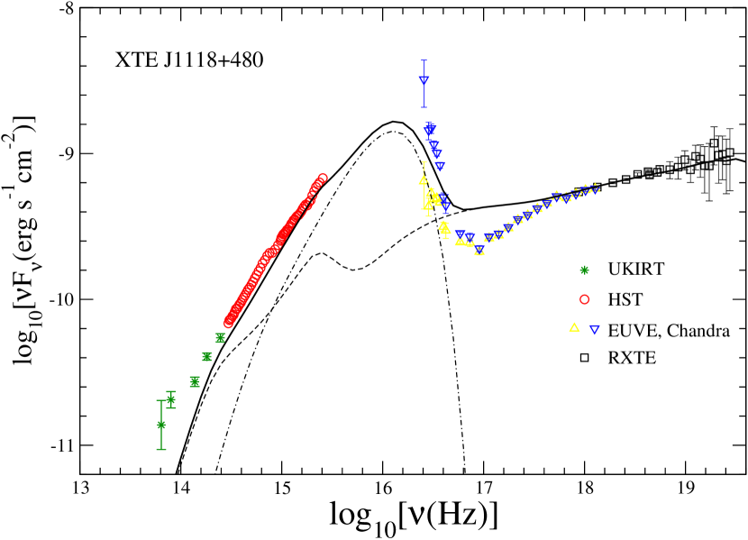
For clarity, we briefly summarize the main observational results here. These include two aspects—spectral and timing features. The most complete spectral energy distribution (SED) of XTE J1118+480 is shown in Figures 1 and 2. The radio data are from Fender et al. (2001) and the infrared to X-ray data from McClintock et al. (2001) (all the data are associated with “epoch 2”, when the best simultaneous coverages were achieved; see Chaty et al. 2003 for a summary of all observations). The radio spectrum is well described by a power-law of the form . Such a spectrum is often thought to be typical of jet emission, although no jet has been directly imaged, down to a limit of (Fender et al. 2001), where is the distance to the source. Note that we do not include in Figures 1 and 2 an observational data point at 350 GHz (Fender et al. 2001), because this measurement was not done simultaneously with the others. From IR to UV, the spectrum is flat, with the HST spectrum exhibiting emission lines. Also, a Balmer jump is seen in absorption at Hz (Hynes et al. 2000), implying that thermal emission contributes substantially to the optical/UV band. The derived EUV spectrum depends sensitively on the assumed , which is still not well constrained but probably lies in the range (McClintock et al. 2001b, 2004). We take this uncertainty into account by requiring the model to stay within the allowed range at EUV energies. McClintock et al. (2001b) fitted the X-ray spectrum with a broken power-law. Above keV they obtained a photon index of , but below keV the spectrum appeared to be relatively harder. However, calibration issues were subsequently noted for the ACIS detectors used in the Chandra observations111 see http://cxc.harvard.edu/cal/Acis/Cal_prods/qeDeg/index.html.. This makes the spectrum uncertain at low energies. There is, in fact, independent evidence that the break at 2 keV may not be real. XTE J1118+480 was observed many times with BeppoSAX, but the X-ray spectra show no apparent deviation from a single power-law at low energies (Frontera et al. 2001).
The main timing features include the following. 1) A quasi-periodic oscillation (QPO) feature was detected in the X-ray light curve, initially at a frequency Hz (Revnitsev, Sunyaev, & Borozdin 2000), and was subsequently found to evolve (Wood et al. 2000). The QPO was also detected in the optical and UV bands at similar frequencies (Haswell et al. 2000; Yamaoka, Ueda & Dotani 2000). The fractional rms amplitude of the QPO is % in the X-ray but only about 1% at UV wavelengths (Hynes et al. 2003, hereafter H03). The fact that the same QPO frequency is seen at optical, UV, and X-ray wavelengths indicates a common origin. 2) XTE J1118+480 also shows rapid aperiodic variability at most wavelengths. The variability amplitude is quite large both in the X-ray and IR bands but is small in the optical/UV band. 3) Correlation between emission at different wavelengths is apparent (H03). In particular, cross-correlation analysis has revealed some puzzling details in the correlation between the optical and X-ray emission (Kanbach et al. 2001; H03; Malzac et al. 2003). In general, the optical photons appear to lag the X-ray photons by s (see H03, though with caveats). The lags are wavelength dependent; on average a longer delay is seen at longer wavelengths. On the other hand, the cross-correlation function (CCF) also shows a “precognition dip”, i.e., the optical emission decreases about seconds before the corresponding X-ray increase (Kanbach et al. 2001). At UV wavelengths the “dip” appears to be weaker and the lag becomes shorter, s (H03). These complicated positive and negative time lags between optical/UV and X-ray emission are not easy to understand. What is quite clear from the derived autocorrelation functions (ACFs) is that the optical/UV emission is not consistent with being due to the re-processing of X-ray photons by the accretion disk, as is often assumed, because the ACF at optical/UV wavelengths is narrower than that in X-rays (Kanbach et al. 2001; Spruit & Kanbach 2002; H03).
Several models have been proposed to explain the observed spectral and temporal properties of XTE J1118+480. Esin et al. (2001, hereafter E01) explain the spectrum with an advection-dominated accretion flow (ADAF) model, based on the work of Narayan (1996) and Esin, McClintock, & Narayan (1997). They assume that the gas lost from the secondary initially forms a standard thin disk outside a transition radius . At , the cool disk is truncated and makes a transition to a hot accretion flow, described as an ADAF (Narayan & Yi 1994, 1995b; Narayan, Mahadevan & Quataert 1998). E01 satisfactorily explain the X-ray, EUV and UV spectra of the source, but their model slightly under-predicts the optical flux and significantly under-predicts the IR fluxes. They do not include radio measurements in their work, but it is quite clear that their model cannot account for the emission at radio wavelengths.
In contrast, Markoff, Falcke, & Fender (2001) propose that the SED of XTE J1118+480 is dominated by synchrotron radiation from a jet, although they also need a truncated accretion disk to explain the UV and EUV spectra. Inside the truncation radius, they assume that the accretion flow becomes an ADAF-like accretion flow. However, unlike E01, they ignore the radiation from the ADAF.
No attempts have been made to explain the observed timing properties with either of the above models. Merloni, Di Matteo & Fabian (2000) consider both spectral and timing data in their work, but their magnetic flare model predicts that the disk emission should peak at about keV, which is in disagreement with the EUVE and Chandra data. Also, the model implies almost no time lag between optical and X-ray photons, which seems to be at odds with the measurements. Recently, Malzac, Merloni & Fabian (2004) have proposed a time dependent, coupled disk-jet model for XTE J1118+480, which has some resemblance to the model we discuss in this paper. Whereas our model attempts to fit the spectral data (see the following sections), Malzac et al. concentrate on understanding the timing features. As pointed out by them, due to the complexity of the time evolution of the accretion-jet system, detailed modeling is impossible. They thus adopt a phenomenological approach. They model the variability by assuming random fluctuations of the output power from the disk and the jet, with the power being injected from a reservoir of stored magnetic field. By carefully choosing their parameters, they are able to reproduce almost all the observed timing features. These parameters can, in principle, constrain the dynamics and geometry of the accretion flow. One of their interesting results is that they can rule out models in which the energy budget is completely dominated by either the jet or the accretion flow; rather, they favor a model in which both components contribute.
In the present paper, we describe a coupled accretion-jet model to simultaneously account for both the spectral and timing properties of XTE J1118+480. We propose that the X-ray spectrum is produced mainly by the ADAF-like hot accretion flow, whereas the radiation at longer wavelengths comes from a jet (as in AGN). A similar idea has been suggested previously (e.g., Hynes et al. 2000; McClintock et al. 2001; Chaty et al. 2003). In § 2, we describe the model and discuss how it can explain the SED of XTE J1118+480. In § 3, we show that the observed temporal properties can also be accommodated qualitatively within the model. We conclude in §4 with a summary and discussion. We present in the Appendix technical details on calculating the jet emission.
2 Fitting the Spectrum
2.1 Accretion flow
The accretion component of our model is implemented in nearly the same manner as in E01, i.e., the accretion flow consists of an inner ADAF and an outer thin disk. However, we have taken into account advances in our understanding of the ADAF during the past ten years. First, both numerical simulations (Stone, Pringle, & Begelman 1999; Hawley & Balbus 2002; Igumenshchev et al. 2003) and analytical work (Narayan & Yi 1994, 1995a; Blandford & Begelman 1999; Narayan et al. 2000; Quataert & Gruzinov 2000) indicate that probably only a fraction of the gas that is available at large radius actually accretes onto the black hole. The rest of the gas is either ejected from the flow or is prevented from being accreted by convective motions. The details are likely to depend on the accretion rate.
We note that the outflow (and convection) is ultimately the result of the accreting gas acquiring a positive Bernoulli parameter, as emphasized by Narayan & Yi (1994, 1995a). Further, the effect is strongest when the accretion rate is much below the threshold above which ADAF ceases to exist. Thus, accretion flows in highly under-luminous sources, like Sgr A* or quiescent X-ray binaries, are expected to have strong outflows. On the other hand, the Bernoulli parameter decreases with increasing radiative efficiency, and in fact becomes negative when the radiative efficiency is large enough. Therefore, for more luminous systems like XTE J1118+480 in outburst and other X-ray binaries in the low/hard state, which have relatively high accretion rates and radiate fairly efficiently, we expect outflows and convection to be less well-developed. In the present paper, we allow for this effect by adopting the following phenomenological prescription for the change in mass accretion rate as a function of radius. We assume that, in the hot flow,
| (1) |
where
| (2a) | |||
| (2b) |
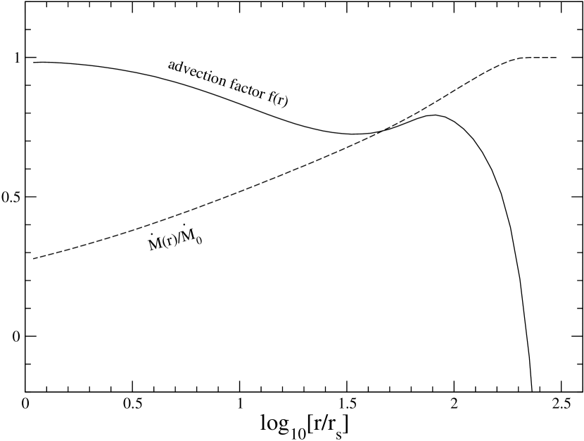
Here is a constant, which we set to , as suggested by our previous modeling of the highly advection-dominated source Sgr A* (Yuan, Quataert & Narayan 2003). The parameter is the advection factor of the accretion flow, defined as
| (3) |
where and are the rates of energy advection, viscous heating, and Coulomb collision cooling for the ions, respectively. When the accretion rate is very low, as in the case of Sgr A*, , so and . In this case, from eq. (1) we have the usual form, , where is the accretion rate at the transition radius (or the outer boundary of the ADAF). We adopt , as in the case of Sgr A* because the physics of the outflow should be the same as long as even though the accretion rates (in Eddington units) can be quite different. We should note, however, that our results are not sensitive to the exact value of .
A negative value of in eq. (2b) means that advection plays a heating rather than a cooling role. In this case, the hot accretion flow is described by a luminous hot accretion flow (hereafter LHAF) model, which is a natural extension of an ADAF to higher accretion rates (Yuan 2001, 2003). From ADAF to LHAF, both and the radiative efficiency increase continuously and smoothly. Yuan & Zdziarski (2004) argue that for luminous X-ray sources, such as the low/hard states of some BHCs and Seyfert 1 galaxies, the luminosity may be above the highest luminosity an ADAF can reach but could be accommodated by an LHAF. We allow for an LHAF in this work, because it is unclear at present which solution, ADAF or LHAF, applies to XTE J1118+480. We simply refer to both the ADAF and LHAF solutions as hot accretion flows.
We calculate the global solution of the hot accretion flow, starting at and integrating inward. The numerical details may be found in Yuan (2001). One main difference with E01 is that we solve the radiation hydrodynamics equations self-consistently, and thus we obtain the exact value of at each radius. In contrast, E01 used the approximation that has a constant average value at all radii. On the other hand, we treat Comptonization within a local approximation, whereas E01 computed the Comptonization globally using the method described in Narayan, Barret & McClintock (1997). The radiation processes we consider include bremsstrahlung, synchrotron emission, and the Comptonization of both synchrotron photons from the hot accretion flow and soft photons from the cool disk outside . The emission from the outer cool disk is modeled as a multicolor blackbody spectrum. The effective temperature as a function of radius is determined by the viscous dissipation and the irradiation of the disk by the inner hot flow.
Yuan & Zdziarski (2004) found that to explain the X-ray emission of most black hole X-ray binaries, is required (see also Narayan 1996). We fix and the magnetic parameter (defined as the ratio of the gas pressure to the sum of gas and magnetic pressure) at their “typical” values: , . We set , i.e., of the viscous dissipation heats electrons directly. The exact value of does not affect our results very much since the required to model XTE J1118+480 in outburst is relatively high, so the main heating mechanism for electrons is energy transfer from ions via Coulomb collisions. In this sense , and are not free parameters, though we should emphasize that large uncertainties exist here. We set the mass of the black hole at , the distance to the source at kpc, and the binary inclination (McClintock et al. 2001a; Wagner et al. 2001). Following E01, we estimate the outer radius of the cool disk using Paczyński’s formula (Paczyński 1971): , where is the Schwarzschild radius of the black hole. The free parameters of the accretion flow are the transition radius , the accretion rate at the transition radius , and an outer boundary condition —the temperature of the accretion flow at (Yuan 1999).
Figure 1 shows the spectral fitting results obtained with the accretion flow model. The values of the parameters are: , . The X-ray emission is produced by Comptonization in the hot flow. The main seed photons are from synchrotron emission by the thermal electrons in the hot flow (as assumed in the original ADAF model of Narayan & Yi 1995b), as opposed to the blackbody emission of the thin disk. This is also consistent with the prediction of Wardzinski & Zdziarski (2000) given that XTE J1118+480 is not very luminous. For more luminous sources, the seed photons may be dominated by blackbody emission from the thin disk. The EUV and UV in the model are mostly from the outer thin disk. The fit is satisfactory, although the optical fluxes are slightly under-predicted. The fact that the UV/optical emission is dominated by the thin disk explains the presence of Balmer jump absorption and emission lines and reprocessing features in the data (§1). The IR and radio fluxes are significantly under-predicted, however (ref. Fig. 2). Figure 3 shows the profiles of the advection factor and the fractional mass accretion rate as a function of radii. We see that is positive over much of the flow except near . Since most of the radiation comes from the inner region where , the solution is in the ADAF rather than LHAF regime, consistent with E01. This is because the luminosity of XTE J1118+480 is not high.
While our results are in general agreement with those of E01, there are two noteworthy differences. First, our value of is significantly larger than that of E01 (). This discrepancy is mainly due to two reasons. First, E01 adopted a no-torque boundary condition at while we apply this condition at the marginally stable orbit of the black hole. Second, in E01 the mass accretion rate of the thin disk follows while we simply use . Both differences are related to the physics of the transition of the accretion flow at , which is highly uncertain at present, so it is not clear which approach is more appropriate. As a comparison, in Chaty et al. (2003) who fitted the EUV spectrum, while in Frontera et al. (2001; 2003) who fitted the iron line and reflection features. The second difference between our model and E01 is that the value of in E01 () is significantly smaller than ours (). This is primarily because (1) we include an outflow in our calculations so that the accretion rate in the inner region is smaller than that at (see Fig. 3 where near the black hole in our model, close to E01’s value); and (2) we use the pseudo-Newtonian potential of Paczyński & Wiita (1980), while E01 used the general relativistic solution of Popham & Gammie (1998) in calculating the radial velocity of the accretion flow. As shown by Narayan et al. (1998), the latter gives higher luminosity for the same accretion rate.
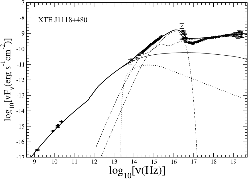
To account for the under-prediction of the IR and radio fluxes, we first consider the effect of nonthermal electrons in the hot accretion flow. Since the inflowing gas is collisionless, processes such as MHD turbulence, reconnection, and weak shocks can accelerate electrons and generate a nonthermal tail at high energies in the electron distribution function. Yuan, Quataert & Narayan (2003) found that the radio spectrum of Sgr A*, which was under-predicted by a pure ADAF model with only thermal electrons, can be explained if roughly of the electron energy is in nonthermal electrons. We tested this idea for XTE J1118+480. The dotted line in Figure 2 shows the (absorbed) synchrotron emission from nonthermal electrons. We see that there is a sharp cut-off below about Hz, so that the emission from nonthermal electrons is unable to fit the radio and IR fluxes. This result is not sensitive to how much energy the nonthermal electrons have. In the case of Sgr A*, the emission from nonthermal electrons extends to much lower frequency and forms a power-law spectrum. The difference between Sgr A* and XTE J1118+480 is that in the latter case the density is several orders of magnitude higher. Therefore, the magnetic field in XTE J1118+480 is much stronger and the lowest frequency that the power-law electrons emit is much higher. We conclude that the accretion flow alone cannot account for the low-frequency spectrum of XTE J1118+480 at radio and IR wavelengths. Some other component, most likely a jet, is required.
2.2 Coupled Accretion-Jet Model
Jets are thought to occur in the low/hard state of BHCs (see Fender 2004 for a review). There have been many papers on the emission of radio jets in active galactic nuclei (e.g., Blandford & Königl 1979; Ghisellini, Maraschi, & Treves 1985; Falcke 1996). In the present paper, following Spada et al. (2001), we adopt the internal shock scenario widely used in interpreting gamma-ray burst (GRB) afterglows (e.g., Piran 1999). The details of the model of the jet radiation are described in Appendix A. Briefly, we assume that, near the black hole, a fraction of the accretion flow is transferred into the vertical direction to form a jet. Since the radial velocity of the accretion flow near the black hole is supersonic, a standing shock should occur at the bottom of the jet due to the bending. From the shock jump conditions, we calculate the properties of the postshock flow, such as the electron temperature . We assume a constant in the jet, which is clearly over-simplified, since adiabatic expansion will cause the electrons to cool. However, the assumption has very little effect on the results because the jet emission is dominated by the nonthermal electrons discussed below. We assume that the jet has a conical geometry with half opening angle , and that the bulk Lorenz factor of the jet is independent of distance from the black hole. We further assume that internal shocks occur due to the collision of shells with different . These shocks accelerate a fraction of the electrons into a power-law energy distribution with index (e.g., Kirk et al. 2000). The steady state energy distribution of the accelerated electrons is carefully determined since it is important for calculating the emitted spectrum. The effect of radiative cooling is considered in this process. Following the widely adopted approach in the study of GRBs, we specify the energy density of accelerated electrons and amplified magnetic field by two free parameters, and . We then calculate the radiative transfer by both thermal and power-law electrons in the jet, although we find that the latter plays a dominant role. Only synchrotron emission is considered since Compton scattering is not important in this case (see also Markoff, Fender & Falcke 2001).
The thin solid line in Figure 2 shows the emission of the jet. The parameters are: mass loss rate in the jet , which is about of the accretion rate in the accretion disk, , , , bulk Lorenz factor of the jet , and length of the jet AU. The values of and are well within the typical range obtained in GRB afterglows (e.g., Panaitescu & Kumar 2001; 2002), and the length of the jet is consistent with the observed upper limit of AU. The value of is well within the range obtained by combining observations and numerical simulations: (Gallo, Fender & Pooley 2003). We see from Figure 2 that the jet emission fits the low-frequency radiation very well. The IR flux is dominated by the jet, while from optical to UV, the jet becomes less important. The contribution of the jet to EUV and X-rays is negligible. We should point out that the solution shown is not unique and that the jet parameters are not as well constrained as those of the accretion flow. However, the results are not very sensitive to the values of the jet parameters.
It is interesting to check whether a pure thermal jet can also explain the data. We find that we can get an equally good fit to the spectrum if we adjust the geometry and profile of the jet carefully. In this model, we only need a tiny fraction of the gas in the accretion flow, , to go into the jet. However, the required temperature is very high, K. In addition, the jet velocity has to be very low, ; otherwise, the required magnetic field in the jet becomes unrealistically large. Such a low speed close to the black hole seems unphysical.
3 Interpreting the Timing Features
3.1 QPOs
Numerous models have been proposed to explain the QPO phenomenon in X-ray binaries (see review by van der Klis 2000). In some models, the QPO frequency is associated with the Keplerian frequency of the accretion flow at a special radius—the transition radius in our case. For example, Giannios & Spruit (2004; see also Rezzolla et al. 2003) suggest that the QPO can be excited by the interaction of the inner hot accretion flow and outer thin disk. The QPOs then result from the basic p-mode oscillations of the inner hot accretion flow, with frequency roughly equal to the Keplerian frequency at . The Keplerian frequency at is Hz, which is roughly consistent with the observed QPO frequency of Hz. Because the entire region of the hot flow oscillates collectively at the same frequency, and the emission from the hot flow contributes somewhat at both optical/UV and X-ray (see Fig. 1), the QPO should be observable at both optical/UV and X-ray wavelengths with the same frequency. Wood et al. (2000) find that the QPO frequency in XTE J1118+480 increases from 0.07 to 0.15 Hz during the outburst, while the 2-10 keV X-ray flux slowly rises and then decreases. Our calculations do not show such a non-monotonic relationship, so the evolution of the QPO remains a puzzle. We should emphasize that the non-monotonic change of the QPO frequency with the flux is not universal among BHCs. In fact, for most sources, the correlation seems to be monotonic (e.g., Cui et al. 1999).
3.2 Variability amplitude
The variability amplitude from the jet is expected to be large, both from internal shocks and from possible instabilities in the jet. The hot accretion flow is thermally marginally unstable, so any perturbations in it will survive and move inward, as shown by numerical simulations (Manmoto et al. 1996) and analytical work (Yuan 2003). However, the growth timescale of the perturbations is longer than the accretion timescale, so the hot accretion flow is not threatened by the instability. The simulations further show that the simulated flux variation can account for the observed substantial variability observed in BHCs. On the other hand, the intrinsic variability of emission from the thin disk should be very weak because the characteristic timescale is many hours even at , i.e., much longer than the observed seconds or minutes variability timescale (e.g., Kanbach et al. 2001). The only source of variability of the thin disk emission is due to the reprocessing of the variable X-ray radiation, but the contribution of this component is very weak.
With the above knowledge, we can qualitatively understand variability amplitudes at different wavelengths. Large variability in the IR and X-ray bands is natural because the IR emission is dominated by the jet and the X-ray emission by the hot flow. As the emission from the disk becomes more important in the optical and UV, the source varies less in these bands. The correlation between optical/UV and X-ray is easily understood because the hot accretion flow contributes in both bands. H03 find that the spectral energy distribution (SED) of the variable component of the emission is roughly a power law, which they argued as being consistent with optically thin synchrotron radiation. However, given the fact that the rms amplitudes were derived from light curves with the same time resolution, it is actually not straightforward to interpret the result, since the intrinsic variability timescale at different wavelengths should be quite different. Moreover, the physical origin of the variability is likely to be complicated (e.g., Malzac, Merloni, & Fabian 2004). We note that a power-law SED of the variability does not arise naturally in a pure jet model (e.g., Markoff, Falcke & Fender 1999). For instance, if we assume that the variability is caused by fluctuations in , such a model would predict a power-law index of , which is the same as the X-ray spectral index, while the measured index of the variability spectrum is (H03).
3.3 Correlations between optical/UV and X-ray
Suppose there is a perturbation due to an instantaneous increase of . The X-ray flux will increase. The increase in will propagate inward with the accretion flow, and eventually will lead to an increase in the mass loss rate and thus the optical/UV emission from the jet. This could explain why the optical/UV variability lags the X-ray variability. Quantitatively, we find that in our model the optical/UV emission from the jet comes mainly from regions at a distance of about from the black hole. This corresponds to a propagation time of s, consistent with the measured s lag. The size of the optical emission region is , where is the half opening angle of the jet. The corresponding light crossing time is s, consistent with the shortest variability timescale ms seen in the optical (e.g., Kanbach et al. 2001). Since the emission at longer wavelengths originates from regions farther away, the time lag should increase with increasing wavelength.
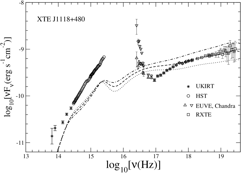
As for the negative lag, we note that, for the parameters of our model (Fig. 1), an increase of in the hot accretion flow results in a decrease of the optical/UV flux, as shown in Figure 4. The optical/UV emission from the hot accretion flow is mainly due to self-absorbed synchrotron emission, which depends on the profiles of and optical depth . For our model, an increase in causes a decrease in the flux. In our model, the optical emission comes from , the UV from , and the X-rays from . So when increases, the optical flux will first decrease, then the UV will decrease, and finally the X-ray flux will increase. This might be the origin of the negative lag of the optical/UV, as well as the negative correlation, and may also explain why the lag in the UV is shorter than in the optical. Since the emission from the hot accretion flow contributes less at shorter wavelengths in the optical/UV regime (see Fig. 1), we can also understand why the dip becomes weaker at shorter wavelengths. Since the IR flux from the hot accretion flow does not vary with varying (see Fig. 4), we predict that such a negative lag should be absent between IR and X-ray.
Quantitatively, however, we are not able to account for the magnitude of the negative lags. The viscous timescale at is s, which is more than 20 times smaller than the observed s negative lag seen in the optical. This might be due to an approximation in the outer boundary condition we assume for the global solution. For technical reasons, we set the angular velocity of the flow at to be substantially sub-Keplerian, , even though it should be super-Keplerian (Abramowicz, Igumenshchev, & Lasota 1998); otherwise, the viscous dissipation would be negative. and the solution would be unphysical (see also Manmoto, Mineshige, & Kusunose 1997). Since the centrifugal force is the dominant factor determining the radial velocity of the accretion flow, our approximation makes the radial velocity much larger than it should actually be and thus lead to a shorter viscous timescale. In addition, the viscosity parameter may be smaller than the value we adopted, which will again result in a longer viscous timescale.
Finally, we note that an increase of in the cool thin disk will obviously result in an increase in the optical/UV emission. However, such an increase is unlikely to be seen in the cross-correlation analysis, since the accretion timescale in the thin disk is on the order of hours.
4 Summary and Discussion
The observational data on XTE J1118+480 is almost unique among all current BHCs. The spectral and timing information impose very strong constraints on theoretical models and provide us with an opportunity to understand in detail the inflow/outflow processes around black holes. In this paper we explain how these observations can be understood in the context of a coupled accretion-jet model. In our model, the accretion flow is described as a geometrically thin cool disk outside a transition radius and a geometrically-thick hot accretion flow inside , as in the model of E01. We adopt a phenomenological prescription for the magnitude of the mass outflow from the hot accretion flow (eqs. 1–3). The free parameters describing the accretion flow are the transition radius , the mass accretion rate at , , and the outer boundary condition at . The spectrum due to the accretion flow alone is shown in Figure 1. The X-ray emission is dominated by Comptonization of synchrotron photons in the hot accretion flow, and both the EUV and UV are dominated by the cool disk. The fit is quite satisfactory in these bands. The optical flux is slightly under-predicted, however, and the IR and radio spectra are significantly under-predicted (Fig. 2). These results are very similar to those of E01.
Obviously, we require an additional component in the model to explain the IR and radio fluxes. We first consider the possibility of nonthermal electrons in the hot accretion flow, but find that this idea does not work. We stress, however, that the failure does not mean that there are no non-thermal electrons in hot accretion flows. Such electrons might, for instance, be responsible for the “hard tail” in the spectrum of Cyg X-1 in the low/hard state (McConnell et al. 2000).
Having eliminated non-thermal electrons as an explanation for the low frequency emission of XTE J1118+480, we argue that the radiation must originate in a jet. Assuming that a small fraction of the mass in the accretion flow is transferred to the jet, we calculate the jet emission using the internal shock scenario that is widely adopted in the study of GRB afterglows. The results of the accretion-jet model are shown in Figure 2. We find that the radiation from the jet can account for all of the radio and IR emission and part of the optical/UV emission. The required mass loss rate in the jets is about 0.5% of the accreted matter.
The coupled accretion-jet model not only explains the spectrum, it also qualitatively explains many of the timing features observed in XTE J1118+480. These features include the frequency of QPO; the similarity of the QPO frequency in optical/UV/X-ray bands (§3.1); the dependence of the variability amplitude on wavelength (§3.2); and the positive and negative time lags between optical/UV and X-ray (§3.3). Quantitatively, however, we are not able to account for the magnitude of the negative time lag between X-ray and optical/UV (§3.3).
It is interesting to examine the energetics of the accretion flow and the jet in our model. The total accretion power is and the power lost in the outflow is . The X-ray luminosity emitted by the hot accretion flow is , the optical/UV luminosity emitted by the thin disk is , and the jet power is , which is times . For comparison, Malzac et al. (2004) require to reproduce the main timing features of XTE J1118+480, while Fender et al. (2001) estimate . The luminosity emitted by the jet in our model is , so the radiative efficiency of the jet is , roughly consistent with the estimate of by Fender et al. (2001) but larger than the value of in Malzac et al. (2004). So there are differences in both the value of and the efficiency of the jet between our model and that of Malzac et al. (2004). One reason for the discrepancy is that Malzac et al. assume the optical flux to be completely dominated by synchrotron emission from the jet, while our detailed modeling shows that the contribution from the accretion flow and the jet are comparable in the optical band (Fig. 2). Thus, more power from the jet is required in their model. In addition, the estimated value of in Malzac et al. (2004) is only , which is 4 times smaller than ours. This is because they integrate the jet emission from radio to optical, while in our model, the jet emission extends up to X-rays (ref. Fig. 2).
Assuming to be the accretion power in the inner region of the accretion flow from which most of the X-ray and jet power originate, we see that only is released through the X-ray emission and channeled into the jet, while most of the accretion power is stored in the accretion flow and advected into the black hole. In other words, XTE J1118+480 is radiatively quite inefficient, in agreement with the conclusion of Malzac et al. (2004). The small ratio of the jet power to the accretion power also justifies our approximation that the jet has very little effect on the global solution of the hot accretion flow. We should point out that some uncertainties exist in the above estimations concerning the jet since the jet parameters in our model are not as well constrained as the parameters of the accretion flow.
Several other caveats also need to be mentioned. First, we adopt a pseudo-Newtonian potential rather than the exact general relativistic approach when we calculate the dynamics of the hot accretion flow. Secondly, we adopt a sub-Keplerian angular velocity at the transition radius whereas the rotation here should be super-Keplerian. The main effect of these two approximations is that the radial velocity in the hot flow is larger than it should actually be, and thus the density is smaller than the “correct value”. We believe that most of the effect is absorbed in the accretion rate parameter . But the approximations do affect some quantitative result such as the time lag between optical/UV and X-ray. Thirdly, we have not explored fully the parameter space. The values of several parameters such as and are fixed in our calculations (to 0.3, 0.9 and 0.5, respectively). Investigating their effects in detail by surveying their entire parameter space would be very time-consuming and is beyond the scope of the paper.
The philosophy of this paper is that the hard X-ray emission comes from the hot accretion flow via thermal Comptonization, and that the contribution from the jet is negligible in this band. This is different from the model of Markoff et al. (2001) in which synchrotron radiation from the jet dominates in X-rays. We note that many details of the X-ray observations of BHCs have been successfully explained with a hot accretion flow model (see the review by Zdziarski & Gierliński 2004) and it remains an open question whether the jet model can do equally well. Poutanen & Zdziarski (2002) and Zdziarski et al. (2003) have pointed out some difficulties with the jet proposal. For example, the non-thermal synchrotron emission in this model cannot produce a sharp enough cut off at high energies, and the predicted spectrum is not as hard as the spectra observed in many BHCs. Also, the jet model should yield X-ray variability virtually independent of energy, which is in strong disagreement with the observational data. Finally, it is unclear if the model can explain the various timing features of XTE J1118+480 described in this paper.
Of course for some black hole sources, the emission from the jet dominates over the accretion flow in the X-ray band. BL Lacs are a well-known class of objects where this situation is known to exist. In previous work we have discussed this possibility also for two other sources, Sgr A* and NGC 4258 (Yuan, Markoff, & Falcke 2002; Yuan et al. 2002). In the case of NGC 4258, the jet emission dominates the accretion flow because we require a significant fraction of the accretion flow to be transfered to the jet, , which is more than times higher than in XTE J1118+480. Such a high value perhaps implies that the black hole in NGC 4258 is very rapidly spinning. In the case of Sgr A*, the value of is similar to XTE J1118+480, but the X-ray emission from the jet is comparable to the accretion flow. This is because the accretion rate (in Eddington units) in Sgr A* is much lower. The flux from the accretion flow, which comes from (multi-order scattering) Comptonization radiation, increases much faster with the accretion rate than that from the jet, which is from synchrotron and (one-order scattering) synchrotron-self-Compton emission. Therefore, the ratio of jet to disk flux increases with decreasing Eddington-scaled accretion rate.
Recently a very interesting correlation between radio and X-ray fluxes has been discovered in GX 339-4. The correlation extends over more than three decades in X-ray flux (Corbel et al. 2003). Such a correlation likely exists in other BHCs and even in AGN (Gallo, Fender, & Pooley 2003; Merloni, Heinz & Di Matteo 2003; Falcke, Körding, & Markoff 2004). The correlation is sometimes used as evidence for a jet origin for the X-ray emission of BHCs, e.g., Markoff et al. (2003). However, Heinz (2004; see also Merloni, Heinz & Di Matteo 2003) recently pointed out that if the electron energy spectrum is not too steep and if radiative losses are included, both of which are required by observations, the jet model cannot explain the radio—X-ray correlation. Merloni, Heinz & Di Matteo (2003) further showed that the X-ray emission is unlikely to be produced by radiatively efficient accretion (as in the sandwiched corona+disk geometry); rather, the accretion flow must be radiatively inefficient. Our preliminary investigations indicate that the radio—X-ray correlation can be explained in the context of our accretion-jet model (Yuan & Cui 2004, in preparation).
Appendix A The Internal Shock Model for Jet Radiation
We adopt the internal shock scenario to calculate the emission from the jet, similar to Spada et al. (2001). We are interested only in the time-averaged spectrum. Following Blandford & Königl (1979), we assume the jet is in conical geometry, with semi angle of whose axis makes an angle with the direction of observer. The jet has a constant velocity, characterized by a bulk Lorenz factor of , and has constant plasma temperature. The mass loss rate in the jet is,
| (A1) |
The quantity is the mass density of the jet plasma at distance from the black hole, measured in the jet-comoving frame.
The main assumption in the internal shock scenario is that the central power engine produces energy which is channelled into jets in an intermittent way, thus faster shells will catch up with slower ones and internal shocks are formed in the jet. The minimum distance the shells propagate before collision occurs is (Piran 1999; Spada et al. 2001). Our results are not sensitive to its exact value.
The bulk Lorenz factor of steady jets in BHCs is likely only mildly relativistic (Fender 2004), e.g., from Gallo, Fender & Pooley 2003. In this case, for an adiabatic index of , the energy density of the internal shock is (Piran 1999),
| (A2) |
where is the Lorenz factor of the formed internal shock, is the post-shock number density with is the preshock number density in the jet determined by eq. (A1).
The shock will heat plasma in the jet, generate/amplify the magnetic field, and accelerate a small fraction of electrons into relativistic energy. We assume that the fraction of accelerated electrons in the shock is and fix . Given the uncertainty in shock physics, as the usual approach, we introduce two dimensionless parameters, and , which measure the fraction of the comoving internal energy of the internal shock stored in the accelerated electrons and magnetic field. Obviously, and are not independent.
Assume that the injected electrons after the shock acceleration have a power-law distribution with index ,
| (A3) |
We set , according to the results of relativistic shock acceleration of Bednarz & Ostrowski (1998) and Kirk et al. (2000). In this case (), we have
| (A4) |
Now we calculate the value of . We have,
| (A5) |
where is the internal energy density of the internal shock. From the above equation and the definition of , we can obtain
| (A6) |
The value of is not important if we are not interested in the fitting the X-ray spectrum of XTE J1118+480 with jet emission. When radiative cooling of relativistic electrons is important, as in the present case of XTE J1118+480, the steady distribution of electrons is different from eq. (A3). Defining a “cooling Lorenz factor” at which the radiative timescale is equal to the dynamical timescale at distance in the jet,
| (A7) |
then depending on the relative value of and , there will be two cases for the steady distribution. When , we have,
| (A8a) | |||
| (A8b) |
When , we have,
| (A9a) | |||
| (A9b) |
The magnetic field generated/amplified by the shock is determined by,
| (A10) |
Since most of electrons may still be in thermal distribution, we need to consider their role in emitting and absorbing photons. To this purpose, we need to know their temperature. One constraint comes from the following consideration. If the jet is formed at the innermost region of the accretion flow, within the sonic point at , since the accretion flow is supersonic, when it is bended into the vertical direction to form the jet, a standing shock should occur. Note that the global solution of ADAF (e.g., Narayan, Kato & Honma 1997) does not find shocks. Our assumption of the bending shock is not in conflict with this result since jet was not considered in that calculation. On the other hand, shock is found in the general relativistic MHD numerical simulations of jet formation (e.g., Koide et al. 2000). ¿From the global solution of the accretion flow, we know the values of preshock quantities. Applying the shock jump conditions at the jet radius, we then be able to calculate the postshock quantities, including the electron temperature (see Yuan, Markoff, & Falcke 2002 for details). Adiabatic expansion will cause the electrons to cool while the internal shocks in the jet will further heat the electrons. But for simplicity, we do not consider these effects, since we find the radiation from the power-law electrons dominate over that from thermal ones.
Now we are ready to calculate the emission from the jet. The emissivity from each location in the jet is,
| (A11) |
where is the optical depth along the line of sight in the jet, is the source function, including the emission and absorption from both thermal () and power-law () electrons in the jet. We then integrate the emission from different distance in the jet to obtain the total emission. The relativistic effects is taken into account in the calculation. There is a remaining important point when we do the integration, that is, we should not integrate all of the volume of the jet. A “volume filling factor” should be introduced. The value of is very uncertain. It obviously depends on the “spatial density” of the internal shocks in the jet. In addition, the generated/amplified magnetic field in the shock may survive for only a short time, this will further decease its value. We set in our model. Fortunately this value is not very important since it can be absorbed in .
References
- (1) Abramowicz, M.A., Igumenshchev, I.V., Lasota, J.-P. 1998, MNRAS, 293, 443
- (2) Bednarz, J., & Ostrowski, M. 1998, PhRvL, 80, 3911
- (3) Blandford, R.D., Begelman, M.C., 1999, MNRAS, 303, L1
- (4) Blandford, R.D., Königl, A. 1979, ApJ, 232, 34
- (5) Chaty, S., Haswell, C.A., Malzac, J., Hynes, R.I., Shrader, C. R., Cui, W. 2003, MNRAS, 346, 689
- (6) Cui, W., Zhang, S.N., Chen, W., & Morgan, E.H. 1999, ApJ, 512, L43
- (7) Done, C., Gierliński, M., 2003, MNRAS, 342, 1041
- (8) Esin, A.A., McClintock, J.E., Drake, J.J., Garcia, M.R., Haswell, C.A., Hynes, R.I., Muno, M.P., 2001, ApJ, 555, 483 (E01)
- (9) Esin, A. A., McClintock, J. E., & Narayan, R. 1997, ApJ, 489, 865
- (10) Falcke, H. 1996, ApJ, 464, L67
- (11) Falcke, H., Körding, E., & Markoff, S. 2004, A&A, 414, 895
- (12) Fender, R.P. 2001, MNRAS, 322, 31
- (13) Fender, R.P. 2004, To appear in ’Compact Stellar X-Ray Sources’, eds. W.H.G. Lewin and M. van der Klis, Cambridge University Press (astro-ph/0303339)
- (14) Fender, R.P., et al. 2001, MNRAS, 322, L23
- (15) Frontera, F. et al., 2001, ApJ, 561, 1006
- (16) Frontera, F. et al., 2003, ApJ, 592, 1110
- (17) Gallo, E., Fender, R.P., & Pooley G.G. 2003, MNRAS, 344, 60
- (18) Ghisellini, G., Maraschi, L., & Treves, A. 1985, A&A, 146, 204
- (19) Giannios, D., & Spruit, H.C. 2004, A&A, in press (astro-ph/0407474)
- (20) Haswell, C.A., Skillman, D., Patterson, J., Hynes, R.I., Cui, W. Chaty, S. 2000, IAU Circ., 7427
- (21) Hawley, J. F. & Balbus, S. A. 2002, ApJ, 573, 738
- (22) Heinz, S. 2004, MNRAS, in press (astro-ph/0409029)
- (23) Hynes R., Mauche C., Haswell C., Shrader C., Cui W., Chaty S., 2000, ApJ, 539, L37
- (24) Hynes R.I. et al., 2003, MNRAS, 345, 292 (H03)
- (25) Igumenshchev, Narayan, R., & Abramowicz, M. A., 2003, ApJ, 592, 1042
- (26) Kanbach, G., Straubmeier C., Spruit H. C., Belloni T., 2001, Nat, 414, 180
- (27) Kirk, J.G., Guthmann, A.W., Gallant, Y.A., & Achterberg, A.A., 2000, ApJ, 542, 235
- (28) Koide, S., Meier, D.L., Shibata, K, Kudoh, T. 2000, ApJ, 536, 668
- (29) Maccarone T. J., 2003, A&A, 409, 697
- (30) Malzac, J., Belloni, T., Spruit, H.C., Kanbach G. 2003, A&A, 407, 335
- (31) Malzac, J., Merloni, A., Fabian, A. 2004, MNRAS, 351, 253
- (32) Manmoto, T., et al. 1996, ApJ, 464, L135
- (33) Markoff S., Falcke H., Fender R., 2001, A&A, 372, L25
- (34) Markoff S., Nowak, M., Corbel, S., Fender, R., Falcke, H. 2003, A&A, 397, 645
- (35) McClintock J.E., Garcia M.R., Caldwell N., Falco E.E., Garnavich P.M., Zhao P., 2001a, ApJ, 551, L147
- (36) McClintock J.E. et al., 2001b, ApJ, 555, 477
- (37) McClintock J.E. et al., 2003, ApJ, 593, 435
- (38) McClintock J.E., Narayan, R., Rybicki, G.B. 2004, ApJ, in press (astro-ph/0403251)
- (39) McClintock J.E. & Remillard, R.A. 2004, to appear as Chapter 4 in ”Compact Stellar X-ray Sources,” eds. W.H.G. Lewin and M. van der Klis, Cambridge University Press (astro-ph/0306213)
- (40) McConnell, M.L. et al. 2000, ApJ, 543, 928
- (41) Merloni A., Di Matteo T., Fabian A. C., 2000, MNRAS, 318, L15
- (42) Merloni A., Heinz, S., & Di Matteo, T. 2003, MNRAS, 345, 1057
- (43) Narayan, R. 1996, ApJ, 462, 136
- (44) Narayan, R., Barret, D., & McClintock, J. E. 1997, ApJ, 482, 448
- (45) Narayan, R., Igumenshchev, I.V., Abramowicz, M. 2000, ApJ, 539, 798
- (46) Narayan, R., Kato, S., Honma, F. 1997, ApJ, 476, 49
- (47) Narayan, R., Mahadevan, R., & Quataert, E. 1998, in “The Theory of Black Hole Accretion Discs”, eds. M.A. Abramowicz, G. Bjornsson and J.E. Pringle (Cambridge University Press), p148
- (48) Narayan, R., Mahadevan, R., Grindlay, J.E., Popham, R. & Gammie, C., 1998, ApJ, 492, 554
- (49) Narayan R., Yi I., 1994, ApJ, 428, L13
- (50) Narayan R., Yi I., 1995a, ApJ, 444, 231
- (51) Narayan R., Yi I., 1995b, ApJ, 452, 710
- (52) Paczyński, B. 1971, ARA&A, 9, 183
- (53) Paczyński, B., & Wiita, P. J. 1980, A&A, 88, 23
- (54) Panaitescu, A., & Kumar, P. 2001, ApJ, 560, L49
- (55) Panaitescu, A., & Kumar, P. 2002, ApJ, 571, 779
- (56) Piran, T. 1999, Phys. Rep., 314, 575
- (57) Popham, R., & Gammie, C. F. 1998, ApJ, 504, 419
- (58) Poutanen, J. & Zdziarski, A.A. 2002, in “New Views on MICROQUASARS”, the 4th Microquasar Workshop, eds. Ph. Durouchoux, Y. Fuchs and J. Rodriguez, p87
- (59) Quataert, E., & Gruzinov, A. 2000, ApJ, 539, 809
- (60) Remillard, R., Morgan, E., Smith, D., & Smith, E. 2000, IAU Circ. 7389
- (61) Revnivtsev, M., Sunyaev, R., Borozdin, K. 2000, A&A, 361, L37
- (62) Rezzolla, L., Yoshida, S’i., Maccarone, T.J., Zanotti, O. 2003, MNRAS, 344, L37
- (63) Spada, M., Ghisellini, G., Lazzati, D., Celotti, A. 2001, MNRAS, 325, 1559
- (64) Spruit H. C., Kanbach G., 2002, A&A, 391, 225
- (65) Stone, J., Pringle, J., & Begelman, M. 1999, MNRAS, 310, 1002
- (66) van der Klis, M. 2000, ARA&A, 38, 717
- (67) Wagner, R.M., Foltz, C.B., Shahbaz, T., Casares, J., Charles, P.A., Starrfield, S.G., Hewett, P. 2001, ApJ, 556, 42
- (68) Wardzinski, G., Zdziarski, A. A. 2000, MNRAS, 314, 183
- (69) Wood, K.S. et al., 2000, ApJ, 544, 45
- (70) Yamaoka, K., Ueda, Y., Dotani, T. 2000, IAU Circ., 7390
- (71) Yuan, F. 1999, ApJ, 521, L55
- (72) Yuan, F. 2001, MNRAS, 324, 119
- (73) Yuan, F. 2003, ApJ, 594, L99
- (74) Yuan, F., Markoff, S., & Falcke, H. 2002, A&A, 383, 854
- (75) Yuan, F., Markoff, S., Falcke, H., & Biermann, P. L. 2002, A&A, 391, 139
- (76) Yuan, F., Quataert, E., Narayan, R. 2003, ApJ, 598, 301
- (77) Yuan, F., Zdziarski, A. 2004, MNRAS, in press (astro-ph/0401058)
- (78) Zdziarski, A.A., Lubinski, P., Gilfanov, M., Revnivtsev, M. 2003, MNRAS, 342, 355
- (79) Zdziarski, A. A., & Gierliński, M. 2004, in “Stellar-mass, intermediate-mass, and supermassive black holes”, Progress of Theoretical Physics, in press (astro-ph/0403683)