Quintessence and the Transition to an Accelerating Universe

Abstract

The implications of seven popular models of quintessence based on supergravity or M/string theory for the transition from a decelerating to an accelerating universe are explored.

All seven potentials can mimic the $\Lambda$CDM model at low redshifts $0\leq z\leq 5$. However, for a natural range of initial values of the quintessence field, the SUGRA and Polónyi potentials predict a transition redshift $z_{t}\approx 0.5$ for $\Omega_{\Lambda 0}=0.70$, in agreement with the observational value $z_{t}\approx 0.46$ and in mild conflict with the $\Lambda$CDM value $z_{t}=0.67$.

Tables are given for the quintessence potentials for the recent average $\overline{w}_{0}$ of the equation of state parameter, and for $w_{0}$ and $w_{1}$ in the low-$z$ approximation $w\approx w_{0}+w_{1}z$.

It is argued that for the exponential potential $e^{\lambda\varphi}$ to produce a viable present-day cosmology, $\lambda\leq\sqrt{2}$.

A robust, scaled numerical method is presented for simulating the cosmological evolution of the scalar field.

1 Introduction

In the standard $\Lambda$CDM cosmological model, the universe makes a transition from deceleration to acceleration at a redshift $z_{t}=0.67$ for $\Omega_{\Lambda 0}=0.70$. This prediction is to be contrasted with the observational value $z_{t}=0.46\pm 0.13$ from the distance-redshift diagram for type Ia supernovae (SNe Ia) [1]. With further observations, the SNe Ia data may converge to the $\Lambda$CDM value. However the value $z_{t}\approx 0.46$ could be a signal of the effects of a quintessence scalar field, extra spatial dimensions, and/or modifications to general relativity.

For the spatially homogeneous quintessence scalar field $\phi$, define the equation of state parameter $w=w(z)=P_{\phi}/\rho_{\phi}$, where the scalar field pressure $P_{\phi}$ and energy density $\rho_{\phi}$ are given by

$$P_{\phi}=\frac{1}{2}\dot{\phi}^{2}-V(\phi),~{}~{}\rho_{\phi}=\frac{1}{2}\dot{\phi}^{2}+V(\phi).$$ (1)

The SNe Ia observations [1] bound the recent ($z\leq 1.75$) average $\overline{w}_{0}<-0.76$ (95% CL) assuming $\overline{w}_{0}\geq-1$, and measure $z_{t}=0.46\pm 0.13$. Alternatively, the SNe Ia data place bounds $-1<w_{0}<-0.72$ (95% CL) and $w_{1}=0.6\pm 0.5$, where $w(z)\approx w_{0}+w_{1}z$ for $z\stackrel{{\scriptstyle<}}{{\mbox{\scriptsize$\sim$}}}1$. This investigation will explore seven popular models of quintessence (see Table 1), and compare and contrast their predictions for $z_{t}$, $\overline{w}_{0}$, $w_{0}$, and $w_{1}$. These models are basically the ones analyzed in Ref. [2] in terms of dark energy and the fate of the universe (see also Refs. [3, 4]).

We will assume a flat Friedmann-Robertson-Walker universe. In the $\Lambda$CDM model, the total energy density $\rho=\rho_{m}+\rho_{r}+\rho_{\Lambda}=\rho_{c}$, where $\rho_{c}$ is the critical density for a flat universe and $\rho_{m}$, $\rho_{r}$, and $\rho_{\Lambda}$ are the energy densities in (nonrelativistic) matter, radiation, and the cosmological constant respectively. In the quintessence/cold dark matter (QCDM) model, $\rho=\rho_{m}+\rho_{r}+\rho_{\phi}=\rho_{c}$. Ratios of energy densities to the critical density will be denoted by $\Omega_{m}=\rho_{m}/\rho_{c}$, $\Omega_{r}=\rho_{r}/\rho_{c}$, $\Omega_{\Lambda}=\rho_{\Lambda}/\rho_{c}$, and $\Omega_{\phi}=\rho_{\phi}/\rho_{c}$, while ratios of present energy densities to the present critical density will be denoted by $\Omega_{m0}$, $\Omega_{r0}$, $\Omega_{\Lambda 0}$, and $\Omega_{\phi 0}\equiv\Omega_{\Lambda 0}$.

dimensionless $V$	name
$e^{\lambda\varphi}$	exponential
$\cosh(\sqrt{2}\varphi)$	cosh (stable de Sitter)
$2-\cosh(\sqrt{2}\varphi)$	cosh (unstable de Sitter)
$1+\cos(\varphi)$	axion
$\cos(\varphi)$	axion (unstable de Sitter)
$\left[\left(1+\frac{\varphi}{\sqrt{2}}\left(\frac{\varphi}{\sqrt{2}}+\beta\right)\right)^{2}-3\left(\frac{\varphi}{\sqrt{2}}+\beta\right)^{2}\right]e^{\varphi^{2}/2}$	Polónyi
$e^{\varphi^{2}/2}/\varphi^{4}$	SUGRA

Table 1: Quintessence potentials inspired by supergravity or M/string theory. $\varphi=\phi/M_{P}$.

In the $\Lambda$CDM model,

$$z_{t}=\left(\frac{2\Omega_{\Lambda 0}}{\Omega_{m0}}\right)^{1/3}-1.$$ (2)

From WMAP $+$ SDSS [5], $\Omega_{\Lambda 0}$ = 0.71${}^{+0.03}_{-0.05}$. For the $1\sigma$ lower bound on $\Omega_{\Lambda 0}$, $z_{t}$ = 0.57, which is just at the upper $1\sigma$ bound for the measured $z_{t}$. Thus the $\Lambda$CDM model value for $z_{t}$ lies at the boundary of the joint 68% confidence interval of the SNe Ia data. We are here interested, however, in whether quintessence models satisfying the observational bounds on $\overline{w}_{0}$ and $w_{0}$ may be in better agreement with the measured central value for $z_{t}$ and consistent with the 1$\sigma$ limits on $w_{1}$. Of the seven models in Table 1, all but two are very close to the $\Lambda$CDM model values for $z_{t}$ and $w_{1}=0$ (in fact, $z_{t}\geq 0.67$ for $\Omega_{\phi 0}$ = 0.70), while the SUGRA and Polónyi potentials differ qualitatively from the others in their predictions for $z_{t}$ and $w_{1}$, and in a certain natural parameter range agree closely with the observed central values.

All seven potentials can mimic the $\Lambda$CDM model at low redshifts $0\leq z\leq 5$ to well within the observational error bounds. If the SNe Ia data converge to the $\Lambda$CDM value for $z_{t}$, then further restrictions can be placed on the possible initial values for $\phi$ and on parameters in the potentials. For the SUGRA and Polónyi potentials to mimic a cosmological constant at present, the initial values for $\phi$ must be fine tuned; these models can naturally predict $z_{t}\approx 0.5$ for $\Omega_{\Lambda 0}=0.70$.

Ref. [6] gave $w_{0}$ equal to $-0.8$ to $-0.9$ and $w_{1}\approx$ 0.3–0.45 for the SUGRA potential $e^{\varphi^{2}/2}/\varphi^{\alpha}$ for $2\leq\alpha\leq 16$—in agreement with our results for $\alpha=4$ for a range of initial values $0<\varphi_{i}=\phi_{i}/M_{P}\stackrel{{\scriptstyle<}}{{\mbox{\scriptsize$\sim$}}}1$.

Curves for $\Omega_{\phi}$ and $w(z)$ for the cosh, SUGRA ($\varphi_{i}=1$ and $\alpha$ = 11 only), and Polónyi ($\varphi_{i}=-1$ only) potentials were given in Ref. [2]; where they overlap, our results agree with theirs. The main focus here, however, is on the transition redshift, which was not addressed in Ref. [2].

Mention should also be made of Ref. [7], which investigated the implication of a 5D brane world modification of general relativity [8] for the recent acceleration of the universe and found $z_{t}\approx 0.5$.

2 Cosmological Equations

The homogeneous scalar field obeys the Klein-Gordon equation

$$\ddot{\phi}+3H\dot{\phi}=-\frac{dV}{d\phi}\equiv-V_{\phi}.$$ (3)

The Hubble parameter $H$ is related to the scale factor $a$ and the energy densities in matter, radiation, and the quintessence field through the Friedmann equation

$$H^{2}=\left(\frac{\dot{a}}{a}\right)^{2}=\frac{\rho}{3M_{P}^{2}}=\frac{1}{3M_{P}^{2}}\left(\frac{1}{2}\dot{\phi}^{2}+V(\phi)+\rho_{m}+\rho_{r}\right)$$ (4)

where the (reduced) Planck mass $M_{P}=2.4\times 10^{18}$ GeV.

We will use the logarithmic time variable $\tau=\ln(a/a_{0})=-\ln(1+z)$. Note that for de Sitter space $\tau=H_{\Lambda}t$, where $H_{\Lambda}^{2}=\rho_{\Lambda}/(3M_{P}^{2})$, and that $H_{\Lambda}t$ is a useful time variable for the era of $\Lambda$-matter domination (see e.g. Ref. [9]). Also note that for $0\leq z\leq z_{BBN}=10^{10}$, $-23.03\leq\tau\leq 0$, where BBN denotes the era of big-bang nucleosynthesis. (BBN occurs over a range of $z\approx 10^{9}$–$10^{10}$; we will take $z_{BBN}\equiv 10^{10}$.)

For numerical simulations, the cosmological equations should be put into dimensionless form. Eqs. (3) and (4) can be cast in the form of a system of two first-order equations in $\tau$ plus a scaled version of $H$:

$$\overline{H}\varphi^{\prime}=\psi$$ (5)

$$\overline{H}(\psi^{\prime}+3\psi)=-3\overline{V}_{\varphi}$$ (6)

$$\overline{H}^{2}=\frac{1}{6}\psi^{2}+\overline{V}+\overline{\rho}_{m}+\overline{\rho}_{r}$$ (7)

where $\overline{H}=H/H_{0}$, $\varphi=\phi/M_{P}$, $\overline{V}=V/\rho_{c0}$, $\overline{\rho}_{m}=\rho_{m}/\rho_{c0}$, $\overline{\rho}_{r}=\rho_{r}/\rho_{c0}$, and a prime denotes differentiation with respect to $\tau$: $\varphi^{\prime}=d\varphi/d\tau$, etc.

A further scaling may be performed resulting in a set of equations which is numerically more robust, especially before the time of BBN:

$$\tilde{H}\varphi^{\prime}=\tilde{\psi}$$ (8)

$$\tilde{H}(\tilde{\psi}^{\prime}+\tilde{\psi})=-3\tilde{V}_{\varphi}$$ (9)

$$\tilde{H}^{2}=\frac{1}{6}\tilde{\psi}^{2}+\tilde{V}+\tilde{\rho}_{m}+\tilde{\rho}_{r}$$ (10)

where $\tilde{H}=e^{2\tau}H/H_{0}$, $\tilde{\psi}=e^{2\tau}\psi$, $\tilde{V}=e^{4\tau}V/\rho_{c0}$, $\tilde{\rho}_{m}=e^{4\tau}\rho_{m}/\rho_{c0}$, and $\tilde{\rho}_{r}=e^{4\tau}\rho_{r}/\rho_{c0}$.

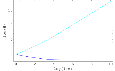
Figure 1: Log₁₀ of $\tilde{H}$ (blue, bottom) vs. $\overline{H}$ (cyan, top) for the $e^{\sqrt{2}\varphi}$ potential.

Figure 1 illustrates (for the exponential potential $e^{\sqrt{2}\varphi}$) that while $\tilde{H}$ varies over only two orders of magnitude between BBN and the present, $\overline{H}$ varies over eighteen orders of magnitude. A similar scaling effect occurs for $\tilde{\psi}$ vs. $\psi$.

We define the recent average of the equation of state parameter $w$ by rewriting the conservation of energy equation

$$\dot{\rho}+3H(\rho+P)=0$$ (11)

where $P$ is the pressure, as

$$0=\rho^{\prime}+3(\rho+P)=\sum_{j}\rho^{\prime}_{j}+3\sum_{j}(1+w_{j})\rho_{j}$$ (12)

where $j$ = $m$, $r$, $\phi$. The solution is

$$\rho_{j}=\rho_{j0}\exp\left\{-3\int_{0}^{\tau}(1+w_{j})d\tau\right\}.$$ (13)

Note that $w_{m}=0$ and $w_{r}=1/3$ are constant except near particle-antiparticle thresholds. The recent average of $w_{\phi}\equiv w$ is defined as

$$\overline{w}_{0}=\frac{1}{\tau}\int_{0}^{\tau}wd\tau.$$ (14)

We will take the upper limit of integration $\tau$ to correspond to $z=1.75$.

Strictly speaking,

$$\rho_{m}=\rho_{m0}e^{-3\tau}f_{m}(\tau),~{}~{}\rho_{r}=\rho_{r0}e^{-4\tau}f_{r}(\tau)$$ (15)

where $f_{m}(\tau)$ and $f_{r}(\tau)$ (with $f_{m}(0)=1=f_{r}(0)$) account for the change in the effective number ${\cal N}(T)$ of massless degrees of freedom as $\tau$ decreases and the temperature $T$ of the gas of relativistic particles increases. Below $T$ = 1 MeV at $z_{BBN}$, ${\cal N}$ = 3.36 is constant, so we can safely set $f_{m}(\tau)=1$ since $\rho_{m}\sim(1+z)^{3}$ quickly becomes negligible compared to $\rho_{r}\sim(1+z)^{4}$ for $z>z_{m-r}$ = 3233 at the equality of matter and radiation densities. In computing the evolution of the quintessence field, we will start with initial conditions at $z_{BBN}$, so we can also set $f_{r}(\tau)=1$ for our purposes. Thus in Eqs. (7) and (10),

$$\overline{\rho}_{m}+\overline{\rho}_{r}=\Omega_{m0}e^{-3\tau}+\Omega_{r0}e^{-4\tau}$$ (16)

$$\tilde{\rho}_{m}+\tilde{\rho}_{r}=\Omega_{m0}e^{\tau}+\Omega_{r0}.$$ (17)

(Ref. [10] suggests the phenomenological form $f_{r}(\tau)=e^{-\tau/15}$ for $z$ going as far back as $10^{30}$.)

The transition redshift $z_{t}$ is defined through the acceleration Friedmann equation

$$\frac{\ddot{a}}{a}=-\frac{1}{6M_{P}^{2}}(\rho+3P)$$ (18)

which may be written in the form

$$-q=\frac{1}{H^{2}}\frac{\ddot{a}}{a}=\frac{H^{\prime}}{H}=-\frac{1}{2}(\Omega_{m}+2\Omega_{r}+(1+3w)\Omega_{\phi})$$ (19)

where $-q$ is the acceleration parameter. The Friedmann equation (4), conservation of energy equation (11), and the acceleration equation (18) are related by the Bianchi identities, so that only two are independent. Eq. (11) gives the evolution (15) of $\rho_{m}$ and $\rho_{r}$, and the Klein-Gordon equation (3) for the weakly coupled scalar field. When a cosmological model involves a collapsing stage where $H$ reverses sign, Eq. (18) should be used instead of Eq. (4). In computational form, the acceleration equation becomes

$$\overline{H}~{}\overline{H}^{\prime}=-\frac{1}{2}\overline{\rho}_{m}-\overline{\rho}_{r}-\frac{1}{3}\psi^{2}+\overline{V}$$ (20)

or

$$\tilde{H}\tilde{H}^{\prime}-2\tilde{H}^{2}=-\frac{1}{2}\tilde{\rho}_{m}-\tilde{\rho}_{r}-\frac{1}{3}\tilde{\psi}^{2}+\tilde{V}.$$ (21)

3 Simulations

For the computations below, we will use Eqs. (8)–(10) with initial conditions specified at $z_{BBN}$ by $\varphi_{i}$ and $\dot{\varphi}_{i}\propto\psi_{i}=0$. The potential $V=A\cdot$(dimensionless potential), where the dimensionless potentials are given in Table 1. The constant $A$ is adjusted by a bisection search method so that $\Omega_{\phi 0}=\Omega_{\Lambda 0}$. This involves the usual single fine tuning.

Since several observational lines including SNe Ia, the cosmic microwave background (CMB), large scale structure (LSS) formation, the integrated Sachs-Wolfe effect, and gravitational lensing measure $0.66\leq\Omega_{\Lambda 0}\leq 0.74$, we will restrict our analysis to this interval, even though technically the bounds are 1$\sigma$. Our main line of development will take $\Omega_{\Lambda 0}=0.70$; in passing, we will make some remarks about what changes if $\Omega_{\Lambda 0}$ = 0.66. The main effect of changing $\Omega_{\Lambda 0}$ to 0.66 (0.74) is to shift the acceleration curves toward the left (right).

We will consider an ultra-light scalar field with $m_{\phi}^{2}\sim H_{\Lambda}^{2}$; then $\phi$ “sits and waits” during the early evolution of the universe, and only starts moving when $H^{2}\sim m_{\phi}^{2}$. In this way it is easy to satisfy the BBN ($z\sim 10^{9}$–$10^{11}$), CMB ($z\sim 10^{3}$–$10^{5}$), and LSS ($z\sim 10$–$10^{4}$) bounds on $\Omega_{\phi}\stackrel{{\scriptstyle<}}{{\mbox{\scriptsize$\sim$}}}0.1$. An ultra-light scalar field also reflects the observational evidence that the universe has only recently made the transition from deceleration to acceleration and has only recently become dominated by dark energy.

Ultra-light scalar fields exist near de Sitter space extrema in 4D extended gauged supergravity theories (with noncompact internal spaces), with quantized mass squared  [11, 12, 3, 13, 14, 15]

$$m^{2}=nH_{\Lambda}^{2},~{}~{}H_{\Lambda}^{2}=\frac{\rho_{\Lambda Q}}{3M_{P}^{2}}$$ (22)

where $-6\leq n\leq 12$ is an integer. In this context $H_{\Lambda}$ is the de Sitter space value of $H$ with effective cosmological constant $\rho_{\Lambda Q}$ at the extremum of the quintessence potential $V$. Note that to produce the current acceleration of the universe, typically $\rho_{\Lambda Q}\approx\rho_{\Lambda}$, but does not equal $\rho_{\Lambda}$ unless the quintessence field—unlike the ones below—is at a de Sitter extremum at $t_{0}$. In certain cases, these theories are directly related to M/string theory. An additional advantage of these theories is that the classical values $m^{2}=nH_{\Lambda}^{2}$ and $\rho_{\Lambda Q}$ are protected against quantum corrections. The relation $m^{2}=nH_{\Lambda}^{2}$ was derived for supergravity with scalar fields; in the presence of other matter fields, the relation may be modified.

3.1 Exponential Potential

The exponential potential $e^{\lambda\varphi}$ [16, 17, 18, 19] can be derived from M-theory [20] or from $N$ = 2, 4D gauged supergravity [21]. The results for $V=Ae^{\lambda\varphi}$ are independent of the initial value $\varphi_{i}$, which we arbitrarily set equal to 1.

$\lambda$	$\overline{w}_{0}$	$z_{t}$	$w_{0}$	$w_{1}$
$1/\sqrt{3}$	$-0.98$	0.68	$-0.95$	$-0.07$
$1$	$-0.93$	0.71	$-0.84$	$-0.19$
$\sqrt{2}$	$-0.83$	0.76	$-0.68$	$-0.33$
$\sqrt{3}$	$-0.70$	0.76	$-0.49$	$-0.40$
$2$	$-0.50$		$-0.27$	$-0.37$

Table 2: Parameters for the potential $e^{\lambda\varphi}$.

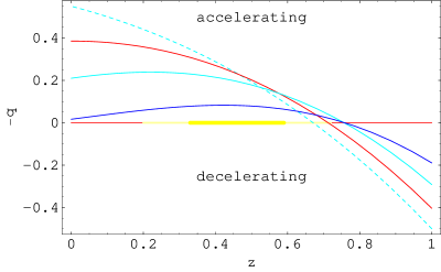
Figure 5: Acceleration parameter $-q$ for the exponential potential $e^{\lambda\varphi}$ (solid) vs. $\Lambda$CDM (dotted). The dark and light yellow lines indicate the 1$\sigma$ and 2$\sigma$ bounds, respectively, on $z_{t}$. $\lambda$ = 1 (red), $\sqrt{2}$ (cyan), and $\sqrt{3}$ (blue) from top to bottom at the left.

For $\lambda^{2}>3$, the cosmological equations have a global attractor with $\Omega_{\phi}=n/\lambda^{2}$, where $n=3$ for the matter dominated era (during which $w=0$) or $n=4$ for the radiation dominated era (during which $w=1/3$). For $\lambda^{2}<3$, the cosmological equations have a late time attractor with $\Omega_{\phi}=1$ and $w=\lambda^{2}/3-1$. In the simulations presented here (see Figs. 2–5 and Table 2), the scalar field is still evolving at $t_{0}$ toward the attractor solution, as advocated in Refs. [22, 23, 2].

For $\lambda=\sqrt{2}$ and $\rho_{m}=0$, $\ddot{a}\rightarrow 0$ asymptotically; if $\rho_{m}>0$, the universe eventually enters a future epoch of deceleration. In either case, there is no event horizon. For $\lambda<\sqrt{2}$, the universe enters a period of eternal acceleration with an event horizon. For $\lambda>\sqrt{2}$, the universe eventually decelerates and there is no event horizon.

The $\Lambda$CDM cosmology is approached for $\lambda\leq 1/\sqrt{3}$. Significant acceleration occurs only for $\lambda\stackrel{{\scriptstyle<}}{{\mbox{\scriptsize$\sim$}}}\sqrt{3}$. For $\lambda=\sqrt{3}$, $w_{0}$ is much too high; setting $\Omega_{\phi 0}=0.66$ still results in $w_{0}=-0.54$. We conclude that $\lambda\leq\sqrt{2}$ in the exponential potential for a viable present-day cosmology.

3.2 Stable de Sitter Cosh Potential

The $\cosh(\sqrt{2}\varphi)$ potential exemplifies $N=2$ supergravity with a future de Sitter space [14, 15], with $m_{\phi}^{2}=6H_{\Lambda}^{2}$.

$\varphi_{i}$	$\overline{w}_{0}$	$z_{t}$	$w_{0}$	$w_{1}$
$0.1$	$-0.998$	0.67	$-0.997$	$0.001$
$0.5$	$-0.96$	0.68	$-0.94$	$0.005$
$1$	$-0.89$	0.72	$-0.81$	$-0.08$
$2$	$-0.84$	0.75	$-0.69$	$-0.30$

Table 3: Parameters for the potential $\cosh(\sqrt{2}\varphi)$.

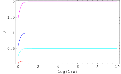
Figure 6: $\varphi(\tau)$ for the potential $\cosh(\sqrt{2}\varphi)$. $\varphi_{i}$ = 0.1 (red), 0.5 (cyan), 1 (blue), and 2 (magenta).

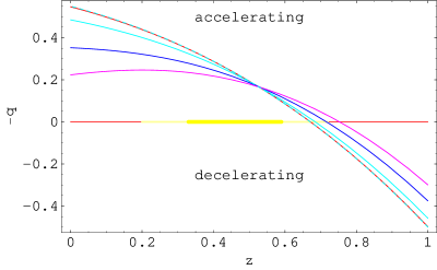
Figure 9: Acceleration parameter $-q$ for the potential $\cosh(\sqrt{2}\varphi)$ (solid) vs. $\Lambda$CDM (dotted). $\varphi_{i}$ = 0.1 (red), 0.5 (cyan), 1 (blue), and 2 (magenta) from top to bottom at the left.

Results for the cosh potential are presented in Figs. 6–9 and Table 3. Near $t_{0}$, $\varphi$ is evolving toward the minimum of the potential. The $\Lambda$CDM model is approached as $\varphi_{i}\rightarrow 0$. For $\varphi_{i}\geq 2$, the $\cosh(\sqrt{2}\varphi)$ results are very nearly the same as for $e^{\sqrt{2}\varphi}$.

3.3 Unstable de Sitter Cosh Potential

The $2-\cosh(\sqrt{2}\varphi)$ potential is derived from M-theory/$N=8$ supergravity [24], with $m_{\phi}^{2}=-6H_{\Lambda}^{2}$ at the maximum of the potential. Near the unstable de Sitter maximum ($\varphi_{i}\rightarrow 0$), the universe can mimic $\Lambda$CDM for a very long time (on the order of or greater than $t_{0}$) [2].

$\varphi_{i}$	$\overline{w}_{0}$	$z_{t}$	$w_{0}$	$w_{1}$
$0.1$	$-0.996$	0.67	$-0.99$	$-0.04$
$0.2$	$-0.98$	0.69	$-0.93$	$-0.24$
$0.3$	$-0.92$	0.77	$-0.64$	$-1.8$

Table 4: Parameters for the potential $2-\cosh(\sqrt{2}\varphi)$.

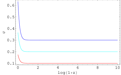
Figure 10: $\varphi(\tau)$ for the potential $2-\cosh(\sqrt{2}\varphi)$. $\varphi_{i}$ = 0.1 (red), 0.2 (cyan), and 0.3 (blue).

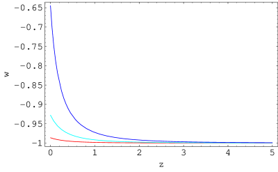
Figure 12: $w$ for the potential $2-\cosh(\sqrt{2}\varphi)$. $\varphi_{i}$ = 0.1 (red), 0.2 (cyan), and 0.3 (blue) from bottom to top.

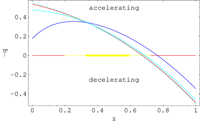
Figure 13: Acceleration parameter $-q$ for the potential $2-\cosh(\sqrt{2}\varphi)$ (solid) vs. $\Lambda$CDM (dotted). $\varphi_{i}$ = 0.1 (red), 0.2 (cyan), and 0.3 (blue) from top to bottom at the left.

Results for the unstable de Sitter cosh potential are presented in Figs. 10–13 and Table 4. The scalar field is just beginning to grow without bound at $t_{0}$. For $\varphi_{i}\geq 0.33$, $\Omega_{\phi 0}$ never reaches 0.70; for $\varphi_{i}\geq 0.35$, $\Omega_{\phi 0}$ never reaches 0.66.

3.4 Axion Potential

For the axion potentials $1+\cos(\lambda\varphi)$ and $\cos(\lambda\varphi)$ in this and the next subsection, we can restrict our attention to $0\leq\lambda\varphi_{i}\leq\pi$. We will set $\lambda=1$; similar results are obtained for $\lambda=\sqrt{2}$.

The axion potential $1+\cos(\varphi)$ is based on $N=1$ supergravity [25, 26], with $m_{\phi}^{2}=3H_{\Lambda}^{2}$. As $\varphi\rightarrow\pi$, the universe evolves to Minkowski space.

$\varphi_{i}/\pi$	$\overline{w}_{0}$	$z_{t}$	$w_{0}$	$w_{1}$
$0.1$	$-0.998$	0.67	$-0.995$	$-0.01$
$0.3$	$-0.98$	0.68	$-0.95$	$-0.10$
$0.5$	$-0.90$	0.75	$-0.74$	$-0.55$
$0.55$	$-0.83$	0.82	$-0.55$	$-1.1$

Table 5: Parameters for the potential $1+\cos(\varphi)$.

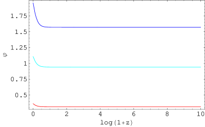
Figure 14: $\varphi(\tau)$ for the potential $1+\cos(\varphi)$. $\varphi_{i}/\pi=0.1$ (red), $0.3$ (cyan), and $0.5$ (blue).

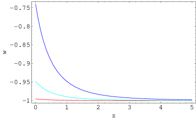
Figure 16: $w$ for the potential $1+\cos(\varphi)$. $\varphi_{i}/\pi=0.1$ (red), $0.3$ (cyan), and $0.5$ (blue) from bottom to top.

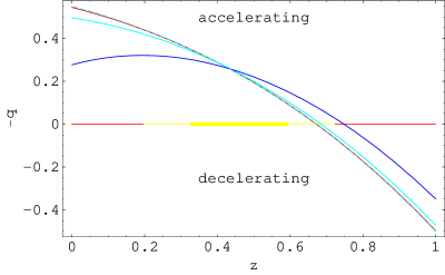
Figure 17: Acceleration parameter $-q$ for the potential $1+\cos(\varphi)$ (solid) vs. $\Lambda$CDM (dotted). $\varphi_{i}/\pi=0.1$ (red), $0.3$ (cyan), and $0.5$ (blue) from top to bottom at the left.

Figures 14–17 and Table 5 present the results for the axion potential. As $\varphi_{i}\rightarrow 0$, a transient de Sitter universe is obtained that mimics the $\Lambda$CDM model for a long time. Near $t_{0}$, $\varphi$ is beginning to evolve toward $\pi$. For $\varphi_{i}/\pi\geq 0.59$, $\Omega_{\phi 0}=0.70$ is never attained; for $\varphi_{i}/\pi>0.61$, $\Omega_{\phi 0}$ never reaches 0.66.

3.5 Unstable de Sitter Axion Potential

The unstable de Sitter axion potential $\cos(\varphi)$ is based on M/string theory reduced to an effective $N=1$ supergravity theory [27], with $m_{\phi}^{2}=-3H_{\Lambda}^{2}$ at the maximum of $V$.

$\varphi_{i}/\pi$	$\overline{w}_{0}$	$z_{t}$	$w_{0}$	$w_{1}$
$0.05$	$-0.998$	0.67	$-0.99$	$-0.01$
$0.10$	$-0.99$	0.68	$-0.98$	$-0.06$
$0.15$	$-0.98$	0.69	$-0.93$	$-0.16$
$0.20$	$-0.94$	0.72	$-0.83$	$-0.47$
$0.25$	$-0.78$	0.94	$-0.16$	$-4.4$

Table 6: Parameters for the potential $\cos(\varphi)$.

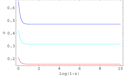
Figure 18: $\varphi(\tau)$ for the potential $\cos(\varphi)$. $\varphi_{i}/\pi=0.05$ (red), $0.1$ (cyan), and $0.15$ (blue).

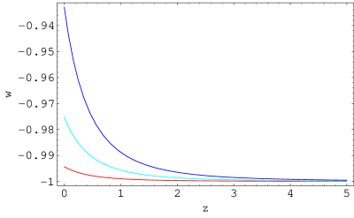
Figure 20: $w$ for the potential $\cos(\varphi)$. $\varphi_{i}/\pi=0.05$ (red), $0.1$ (cyan), and $0.15$ (blue) from bottom to top.

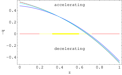
Figure 21: Acceleration parameter $-q$ for the potential $\cos(\varphi)$ (solid) vs. $\Lambda$CDM (dotted). $\varphi_{i}/\pi=0.05$ (red), $0.1$ (cyan), and $0.15$ (blue) from top to bottom at the left.

Results for the unstable axion potential are presented in Figs. 18–21 and Table 6. An unstable de Sitter universe that mimics $\Lambda$CDM for a long time [2] is obtained as $\varphi_{i}\rightarrow 0$. Near $t_{0}$, $\varphi$ is beginning to evolve toward $\pi$. For $\varphi_{i}/\pi=0.25$, there is a transition back to deceleration at $z_{t}=0.12$.

3.6 Polónyi Potential

The Polónyi potential $\left[\left(1+\frac{\varphi}{\sqrt{2}}\left(\frac{\varphi}{\sqrt{2}}+\beta\right)\right)^{2}-3\left(\frac{\varphi}{\sqrt{2}}+\beta\right)^{2}\right]e^{\varphi^{2}/2}$ is derived from $N=1$ supergravity [28] (for a review, see Ref. [29]). The potential is invariant under the transformation $\varphi\rightarrow-\varphi$, $\beta\rightarrow-\beta$.

$\varphi_{i}$	$\overline{w}_{0}$	$z_{t}$	$w_{0}$	$w_{1}$
$0.05$	$-0.85$	0.81	$-0.54$	$-1.7$
$0$	$-0.89$	0.76	$-0.68$	$-0.96$
$-0.5$	$-0.96$	0.69	$-0.91$	$-0.13$
$-1.0$	$-0.92$	0.70	$-0.87$	$-0.07$
$-1.5$	$-0.74$	0.57	$-0.74$	$0.16$
$-1.6$	$-0.69$	0.49	$-0.73$	$0.21$
$-1.7$	$-0.64$	0.43	$-0.72$	$0.26$
$-1.8$	$-0.59$	0.39	$-0.71$	$0.30$
$-1.9$	$-0.56$	0.36	$-0.71$	$0.32$
$-2.0$	$-0.53$	0.36	$-0.72$	$0.32$
$-2.5$	$-0.53$	0.42	$-0.76$	$0.25$

Table 7: Parameters for the Polónyi potential with $\beta=2-\sqrt{3}$.

$\varphi_{i}$	$\overline{w}_{0}$	$z_{t}$	$w_{0}$	$w_{1}$
$-1.5$	$-0.74$	0.55	$-0.77$	$0.21$
$-1.6$	$-0.69$	0.49	$-0.76$	$0.27$
$-1.7$	$-0.64$	0.43	$-0.75$	$0.32$
$-1.8$	$-0.60$	0.40	$-0.75$	$0.35$
$-1.9$	$-0.56$	0.39	$-0.76$	$0.36$
$-2.0$	$-0.54$	0.38	$-0.76$	$0.36$

Table 8: Parameters for the Polónyi potential with $\beta=0.2$.

$\varphi_{i}$	$\overline{w}_{0}$	$z_{t}$	$w_{0}$	$w_{1}$
$-1.5$	$-0.73$	0.58	$-0.68$	$0.02$
$-1.6$	$-0.68$	0.49	$-0.66$	$0.07$
$-1.7$	$-0.63$	0.40	$-0.64$	$0.12$
$-1.8$	$-0.58$	0.35	$-0.63$	$0.15$
$-1.9$	$-0.54$	0.32	$-0.63$	$0.17$
$-2.0$	$-0.51$	0.30	$-0.63$	$0.18$

Table 9: Parameters for the Polónyi potential with $\beta=0.4$.

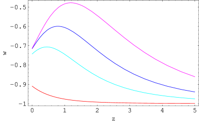
Figure 25: $w$ for the Polónyi potential. $\varphi_{i}=-0.5$ (red), $-1.5$ (cyan), $-1.7$ (blue), and $-1.9$ (magenta) from bottom to top.

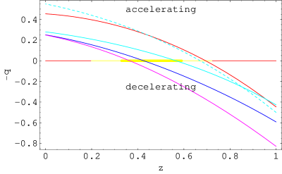
Figure 26: Acceleration parameter $-q$ for the Polónyi potential (solid) vs. $\Lambda$CDM (dotted). $\varphi_{i}=-0.5$ (red), $-1.5$ (cyan), $-1.7$ (blue), and $-1.9$ (magenta) from top to bottom at the left.

Following Ref. [2], we will take $m_{\phi}^{2}\sim\rho_{\Lambda}/M_{P}^{2}$ and set $\beta=2-\sqrt{3}$, 0.2, and 0.4, for which the universe asymptotically evolves to Minkowski space, de Sitter space, or a collapse respectively (see Fig. 22). Figures 23–26 and Table 7 have $\beta=2-\sqrt{3}$. For this value of $\beta$, $\Omega_{\phi 0}=0.70$ is not reached for $\varphi_{i}\geq 0.09$. $\Omega_{\phi}$ begins to violate the LSS bound as $\varphi_{i}$ goes below $-2.5$. The $\Lambda$CDM model is approximated for $\varphi_{i}\approx-0.5$. At $t_{0}$, $\varphi$ is beginning to evolve toward the location $\varphi=\sqrt{2}(\sqrt{3}-1)$ of the minimum of the potential. For $-2.0\stackrel{{\scriptstyle<}}{{\mbox{\scriptsize$\sim$}}}\varphi_{i}\stackrel{{\scriptstyle<}}{{\mbox{\scriptsize$\sim$}}}-1.5$, $z_{t}\approx 0.5$ and at least $w_{0}$ and $w_{1}$ satisfy the observational bounds.

Tables 8 and 9 demonstrate that a transition redshift $z_{t}\approx$ 0.4–0.5 is not an accident due to the particular choice $\beta=2-\sqrt{3}$.

3.7 SUGRA Potential

The SUGRA potential $e^{\varphi^{2}/2}/\varphi^{\alpha}$ is derived from $N=1$ supergravity [30, 31, 6, 32]. The minimum of the potential occurs at $\varphi=\sqrt{\alpha}$, and $m_{\phi}^{2}=6H_{\Lambda}^{2}$. We will take $\alpha=4$, which has the interesting property that the minimum of the potential $V_{min}\sim M^{8}/M_{P}^{4}\sim\rho_{\Lambda}$ for $M\sim M_{weak}\sim$ 1 TeV [6].

$\varphi_{i}$	$\overline{w}_{0}$	$z_{t}$	$w_{0}$	$w_{1}$
$10^{-6}$	$-0.68$	0.50	$-0.86$	$0.35$
$0.1$	$-0.68$	0.50	$-0.86$	$0.35$
$0.5$	$-0.67$	0.50	$-0.86$	$0.36$
$1$	$-0.74$	0.53	$-0.82$	$0.36$
$1.5$	$-0.94$	0.68	$-0.93$	$0.06$
$1.9$	$-0.998$	0.67	$-0.997$	$0.001$
$2.1$	$-0.998$	0.67	$-0.997$	$0.001$
$2.5$	$-0.96$	0.68	$-0.94$	$0.01$
$3$	$-0.85$	0.69	$-0.79$	$0.07$
$3.5$	$-0.65$	0.39	$-0.63$	$0.26$
$4$	$-0.44$	0.14	$-0.57$	$0.53$

Table 10: Parameters for the SUGRA potential.

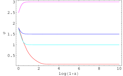
Figure 27: $\varphi(\tau)$ for the SUGRA potential. $\varphi_{i}=0.1$ (red), 1 (cyan), 1.5 (blue), and 3 (magenta).

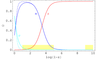
Figure 28: $\Omega$ for the SUGRA potential. $\varphi_{i}=0.1$ (solid) vs. $\Lambda$CDM (dotted).

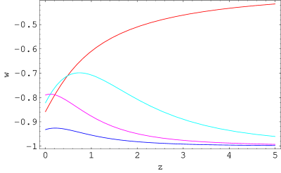
Figure 29: $w$ for the SUGRA potential. $\varphi_{i}=0.1$ (red, top), 1 (cyan, second from top), 1.5 (blue, bottom), and 3 (magenta, third from top) at the right.

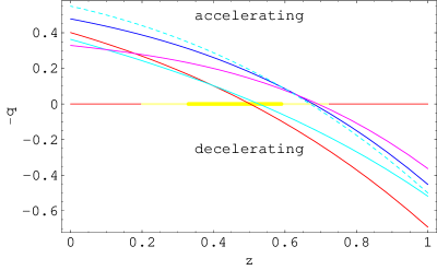
Figure 30: Acceleration parameter $-q$ for the SUGRA potential (solid) vs. $\Lambda$CDM (dotted). $\varphi_{i}=0.1$ (red), 1 (cyan), 1.5 (blue), and 3 (magenta) from bottom to top at the right.

Results for the SUGRA potential are presented in Figs. 27–30 and Table 10. At present $\varphi$ is evolving toward the location of the minimum of the potential. For $\varphi_{i}$ near the minimum of $V$ at $\varphi=2$, the SUGRA potential cosmology approaches $\Lambda$CDM. For $\varphi_{i}\geq 4$, $\overline{w}_{0}$ and $w_{0}$ are much too high.

The transition redshift $z_{t}\approx 0.5$ for $0<\varphi_{i}\stackrel{{\scriptstyle<}}{{\mbox{\scriptsize$\sim$}}}1$. For $0<\varphi_{i}\leq 0.5$, asymptotic values $\overline{w}_{0}=-0.68$, $z_{t}=0.50$, $w_{0}=-0.86$, and $w_{1}=0.35$ are obtained, which makes these SUGRA model values robust. These asymptotic values are in excellent agreement with the observed central values. (There is also a very small interval $\varphi_{i}=3.3$–$3.55$ which yields $z_{t}$ = 0.33–0.59.)

4 Conclusion

All seven potentials can closely mimic the $\Lambda$CDM model at low redshifts, but only the SUGRA and Polónyi potentials can realize a transition redshift of $z_{t}\approx 0.5$ for $\Omega_{\Lambda 0}=0.70$. The other five models predict $z_{t}\geq 0.67$.

The SN Ia central value $z_{t}\approx 0.5$ can naturally be explained either by the SUGRA potential with $0<\varphi_{i}\stackrel{{\scriptstyle<}}{{\mbox{\scriptsize$\sim$}}}1$ or by the Polónyi potential with $-2.0\stackrel{{\scriptstyle<}}{{\mbox{\scriptsize$\sim$}}}\varphi_{i}\stackrel{{\scriptstyle<}}{{\mbox{\scriptsize$\sim$}}}-1.5$. For just the solutions with $z_{t}\approx 0.5$, (i) $\Omega_{\phi}$ becomes significant noticeably earlier than $\Omega_{\Lambda}$ for $\Lambda$CDM and (ii) either $w$ has a maximum near $z=1$ or $w$ evolves rapidly between $z=5$ and the present (SUGRA $0<\varphi_{i}\leq 0.5$). The SUGRA range of initial values does not involve fine tuning, and has the advantage of also offering a explanation (when $\alpha=4$) of the parametric relationship $\rho_{\Lambda}\sim M_{weak}^{8}/M_{P}^{4}$.

The low-$z$ ($0\leq z\leq 5$) data on $z_{t}$, $\overline{w}_{0}$, $w_{0}$, and $w_{1}$, although clearly capable of ruling out a cosmological constant, cannot easily distinguish between the stable and unstable de Sitter cases for the cosh potentials, between the two axion potentials, or among the three different Polónyi potential cases. There is no clear distinguishing signal like the sign of $w_{1}$. However, knowledge of $w(z)$ for $0\leq z\leq 5$ does hold out the prospect—if $\Omega_{\Lambda 0}$ is actually due to quintessence—of determining which quintessence potential nature may have chosen.

Figure 2: $\varphi(\tau)$ for the exponential potential $e^{\lambda\varphi}$. $\lambda$ = 1 (red), $\sqrt{2}$ (cyan), and $\sqrt{3}$ (blue) from top to bottom.

Figure 3: $\Omega$ for the exponential potential $e^{\sqrt{2}\varphi}$ (solid) vs. $\Lambda$CDM (dotted). The light yellow rectangles are the bounds on $\Omega_{\phi}$ from LSS, CMB, and BBN.

Figure 4: $w$ for the exponential potential $e^{\lambda\varphi}$. $\lambda$ = 1 (red), $\sqrt{2}$ (cyan), and $\sqrt{3}$ (blue) from bottom to top.

Figure 7: $\Omega$ for the potential $\cosh(\sqrt{2}\varphi)$, $\varphi_{i}$ = 1 (solid) vs. $\Lambda$CDM (dotted).

Figure 8: $w$ for the potential $\cosh(\sqrt{2}\varphi)$. $\varphi_{i}$ = 0.1 (red), 0.5 (cyan), 1 (blue), and 2 (magenta) from bottom to top.

Figure 11: $\Omega$ for the potential $2-\cosh(\sqrt{2}\varphi)$, $\varphi_{i}$ = 0.2 (solid) vs. $\Lambda$CDM (dotted).

Figure 15: $\Omega$ for the potential $1+\cos(\varphi)$, $\varphi_{i}/\pi=0.3$ (solid) vs. $\Lambda$CDM (dotted).

Figure 19: $\Omega$ for the potential $\cos(\varphi)$, $\varphi_{i}/\pi$ = 0.1 (solid) vs. $\Lambda$CDM (dotted).

Figure 22: Dimensionless Polónyi potential for $\beta=2-\sqrt{3}$ (cyan, $V_{min}=0$), 0.2 (red, $V_{min}>0$), and 0.4 (blue, $V_{min}<0$).

Figure 23: $\varphi(\tau)$ for the Polónyi potential. $\varphi_{i}=-0.5$ (red), $-1.5$ (cyan), $-1.7$ (blue), and $-1.9$ (magenta).

Figure 24: $\Omega$ for the Polónyi potential. $\varphi_{i}=-1.7$ (solid) vs. $\Lambda$CDM (dotted).

References

- [1] A. G. Riess et al. [Supernova Search Team Collaboration], astro-ph/0402512.
- [2] R. Kallosh, A. D. Linde, S. Prokushkin, and M. Shmakova, Phys. Rev. D 66, 123503 (2002), hep-th/0208156.
- [3] R. Kallosh, A. D. Linde, S. Prokushkin, and M. Shmakova, Phys. Rev. D 65, 105016 (2002), hep-th/0110089.
- [4] R. Kallosh and A. D. Linde, Phys. Rev. D 67, 023510 (2003), hep-th/0208157.
- [5] M. Tegmark et al. [SDSS Collaboration], Phys. Rev. D 69, 103501 (2004), astro-ph/0310723.
- [6] P. Brax, J. Martin, and A. Riazuelo, Phys. Rev. D 64, 083505 (2001), hep-ph/0104240.
- [7] J. S. Alcaniz and N. Pires, astro-ph/0404146.
- [8] G. R. Dvali, G. Gabadadze and M. Porrati, Phys. Lett. B 485, 208 (2000), hep-th/0005016.
- [9] C. L. Gardner, Phys. Rev. D 68, 043513 (2003), astro-ph/0305080.
- [10] L. Anchordoqui and H. Goldberg, Phys. Rev. D 68, 083513 (2003), hep-ph/0306084.
- [11] S. J. Gates and B. Zwiebach, Phys. Lett. B 123, 200 (1983).
- [12] C. M. Hull and N. P. Warner, Class. Quant. Grav. 5, 1517 (1988).
- [13] G. W. Gibbons and C. M. Hull, hep-th/0111072.
- [14] P. Fré, M. Trigiante, and A. Van Proeyen, Class. Quant. Grav. 19, 4167 (2002), hep-th/0205119.
- [15] R. Kallosh, hep-th/0205315.
- [16] C. Wetterich, Nucl. Phys. B 302, 668 (1988).
- [17] P. G. Ferreira and M. Joyce, Phys. Rev. D 58, 023503 (1998), astro-ph/9711102.
- [18] E. J. Copeland, A. R. Liddle, and D. Wands, Phys. Rev. D 57, 4686 (1998), gr-qc/9711068.
- [19] M. Doran and C. Wetterich, Nucl. Phys. Proc. Suppl. 124, 57 (2003), astro-ph/0205267.
- [20] P. K. Townsend, JHEP 0111, 042 (2001), hep-th/0110072.
- [21] L. Andrianopoli, M. Bertolini, A. Ceresole, R. D’Auria, S. Ferrara, P. Fré, and T. Magri, J. Geom. Phys. 23, 111 (1997), hep-th/9605032.
- [22] J. Weller and A. Albrecht, Phys. Rev. D 65, 103512 (2002), astro-ph/0106079.
- [23] U. J. Lopes Franca and R. Rosenfeld, JHEP 0210, 015 (2002), astro-ph/0206194.
- [24] C. M. Hull, Class. Quant. Grav. 2, 343 (1985).
- [25] J. A. Frieman, C. T. Hill, A. Stebbins, and I. Waga, Phys. Rev. Lett. 75, 2077 (1995), astro-ph/9505060.
- [26] I. Waga and J. A. Frieman, Phys. Rev. D 62, 043521 (2000), astro-ph/0001354.
- [27] K. Choi, Phys. Rev. D 62, 043509 (2000), hep-ph/9902292.
- [28] J. Polónyi, Hungary Central Inst Res–KFKI-77-93 (1978).
- [29] H. P. Nilles, Phys. Rept. 110, 1 (1984).
- [30] P. Brax and J. Martin, Phys. Lett. B 468, 40 (1999), astro-ph/9905040.
- [31] P. Brax and J. Martin, Phys. Rev. D 61, 103502 (2000), astro-ph/9912046.
- [32] E. J. Copeland, N. J. Nunes, and F. Rosati, Phys. Rev. D 62, 123503 (2000), hep-ph/0005222.