The non-linear evolution of bispectrum from the scale-free N-body simulation

Abstract

We have accurately measured the bispectrum for four scale-free models of structure formation with the spectral index $n=1$, $0$, $-1$, and $-2$. The measurement is based on a new method that can effectively eliminate the alias and numerical artifacts, and reliably extend the analysis into the strongly non-linear regime. The work makes use of a set of state-of-the art N-body simulations that have significantly increased the resolution range compared with the previous studies on the subject. With these measured results, we demonstrate that the measured bispectrum depends on the shape and size of $k$-triangle even in the strongly nonlinear regime. It increases with wavenumber and decreases with the spectral index. These results are in contrast with the hypothesis that the reduced bispectrum is a constant in the strongly non-linear regime. We also show that the fitting formula of Scoccimarro & Frieman (1999) does not describe our simulation results well (with a typical error about 40 percent). In the end, we present a new fitting formula for the reduced bispectrum that is valid for $-2\leq n\leq 0$ with a typical error of $10$ percent only.

1 Introduction

Large-scale structures in the Universe are thought to arise from small primordial fluctuations through gravitational amplification. It is known that gravitational clustering is a non-linear process. When the density fluctuations are sufficiently small, the evolution of the structures can be studied using perturbation theory (PT). With the growth of the fluctuation, even for an initially Gaussian fluctuation, nonlinear gravitational instability induces non-Gaussian signatures in the density field. In the weakly non-linear regime, leading order (tree-level) perturbation theory (Juszkiewicz, Bouchet & Colombi 1993; Bernardeau 1994a; Bernardeau et al. 1994b; Łokas et al. 1995; Gaztañaga & Baugh 1995; Baugh, Gaztañaga & Efstathiou 1995; Bouchet et al. 1995) can describe the clustering properties successfully. As one approaches smaller scales, the loop corrections to the tree-level results are expected to become important (Scoccimarro & Frieman 1996; Scoccimarro 1997). In the non-linear regime, numerical simulations must be applied to follow the development of the cosmic structures.

The n-point correlation functions have been widely used as a powerful tool for quantifying the statistical properties of a density field both in theoretical models and observational catalogs (Peebles 1980). For a Gaussian random field, the two-point correlation function (2PCF) or its Fourier transform, the power spectrum $P(k)$ can completely characterize its statistical properties, with all higher-order (connected) correlation functions being zero. It requires the higher order correlation functions to describe the statistical properties of the non-Gaussian distribution resulting from gravitational instability (Peebles 1980; Fry 1984; Bernardeau et al. 2002 for an excellent review and references therein).

The bispectrum, the three-point correlation function (3PCF) in Fourier space, is the lowest order statistic that probes the shape of large-scale structures generated by the gravitational clustering (Peebles 1980). Theoretical models of weakly non-linear 3PCF have been studied well in the literature based on PT. PT can describe properties of dark matter on large scales $\geq 10\,h^{-1}{\rm{Mpc}}$. It predicts that the 3PCF depends on the shape of the linear power spectrum and on the shape of the triangle configuration both in real space (Jing, Börner & Valdarnini 1995; Jing & Börner 1997; Frieman & Gaztañaga 1999; Barriga & Gaztañaga 2002) and in Fourier space (Fry 1984; Scoccimarro et al. 1998; Scoccimarro et al. 1999). When the galaxy bias is considered, the bispectrum of galaxies contains information on the primordial fluctuation and on galaxy biasing (Fry 1994; Fry & Gaztañaga 1993; Hivon et al. 1995; Mo, Jing, & White 1997; Matarrese et al. 1997; Verde et al. 2002). Measuring the galaxy bispectrum on large scales can help break the degeneracy between the linear bias and the matter parameter $\Omega_{m}$ usually present in the dynamical analysis of galaxy redshift surveys (Fry 1984; Hivon et al. 1995; Matarrese et al. 1997; Verde et al. 1998; Scoccimarro et al. 1998). Several authors have started to measure the bias parameters from current large galaxy surveys (Frieman & Gaztañaga 1999 and Gaztañaga & Freiman 1994 for the APM galaxies; Scoccimarro et al. 2001c for IRAS galaxies; Verde et al. 2002 and Jing & Börner 2003 for the 2dFGRS galaxies; Kayo et al. 2004 for SDSS galaxies).

A quantitative modeling of the 3PCF or bispectrum in the nonlinear regime is more challenging. There have been attempts to predict the 3PCF based on the so-called halo model (Ma & Fry 2000, Scoccimarro et al. 2001b, Takada & Jain 2003a, Wang et al. 2004). In their detailed modeling, Takada & Jain (2003a) found that the halo model prediction for the 3PCF agrees with the simulation result of Jing & Börner (1998) both in linear and strongly non-linear regimes, but fails on intermediate non-linear scales ($\sim 1\,h^{-1}{\rm{Mpc}}$). They also pointed out that the 3PCF at the intermediate scales is very sensitive to the outer radial cut of halos, which could be the reason for the failure of the halo model. On the other hand, N-body simulations have been widely used to study the 3PCF or bispectrum in the nonlinear regime (Davis et al. 1985; Efstathiou et al. 1988). Based on extensive studies with N-body simulations, a fitting formula for the bispectrum was proposed for the scale-free models by Scoccimarro & Frieman(1999, hereafter SF99), and then extended for the cold dark matter (CDM) models by Scoccimarro & Couchman (2001).

The fitting formula of Scoccimarro & Couchman (2001) was applied to calculating the skewness of the convergence field in the weak gravitational lensing survey (Van Waerbeke et al. 2001; Hamana et al. 2002). Nowadays weak lensing surveys have become detailed to start measuring the skewness of the lensing shear field (Pen et al. 2003; Zhang et al. 2003), and will soon become big enough to measure the three-point correlation function of cosmic shears (Schneider et al. 2003; Takada & Jain 2003b). It is important to reliably predict the skewness and the three-point correlation function of cosmic shears in cosmological models, as the observational determinations of these quantities are expected to yield a measure of the cosmological density parameter (Bartelmann & Schneider 2001 for an excellent review). Therefore, the motivation is high to derive an accurate model for the bispectrum from linear to non-linear scales, and present them in a form useful for the weak lensing survey analysis.

In this paper, we present such a study to investigate how the non-linear evolution of the bispectrum proceeds with a set of scale-free simulations of $512^{3}$ particles. The simulations have the initial spectral index $n=1$, $0$, $-1$, or $-2$. We find that the bispectrum depends not only on $n$ but also on the shape and size of the triangle even in the strong non-linear regime. Our results show that the formula of SF99 cannot accurately describe the properties of the bispectrum in the non-linear regime. Comparing our measured non-linear bispectrum with the weakly non-linear bispectrum obtained from the second order PT (hereafter PT2), we have arrived at a new formula for the bispectrum that is significantly more accurate than that of SF99.

In this analysis, we have carefully examined possible effects on the bispectrum measurement of the numerical artifacts, such as finite box size, force softening, and particle discreteness. We have also closely paid attention to the effect caused by the mass assignment using the Fast Fourier Transform (FFT, i.e. the alias effect). In order to get the true power spectrum and bispectrum from the simulation, we have developed a procedure to correct for the numerical and alias effects.

This paper is organized as follows. In section 2, we give a brief overview of the self-similar evolution of the density field. In section 3, we describe the numerical simulations used. In section 4, we introduce the power spectrum and the bispectrum, and outline the possible numerical artifacts in the measurements of the power spectrum and the bispectrum. In section 5, we describe our method to measure the bispectrum. We present the measured bispectrum, and give our fitting formula for the bispectrum in section 6. The last section contains our summary.

2 Self-similarity

Gravitational clustering from initial conditions has provided one of the classic problems in cosmology. To achieve a self-similar evolution, according to Peebles (1980) and Efstathiou et al.(1988), two conditions must be fulfilled: (1) The background cosmology should not contain any characteristic scales, thus the universe must be an Einstein-de Sitter one, and (2) The initial density field should have no characteristic length scale, thus its initial power spectrum must be a power law.

For a self-similar clustering pattern, its physical properties remain the same during its evolution when the length scale $R$ is scaled by a characteristic scale $R_{0}$. A simple choice of $R_{0}$ for a self-similar clustering is the scale at which the fluctuations begin to become non-linear, i.e., the variance of the linear density field smoothed on this scale is unity,

$$\sigma^{2}(R_{0},a)=1\,.$$ (1)

The variance is defined by

$$\sigma^{2}(R,a)=\int\Delta^{2}_{L}(k,a)|W(kR)|^{2}{dk\over k}.$$ (2)

where $W(x)$ is the Fourier transform of a window function(usually a top hat or Gaussian), $\Delta^{2}(k)=d\sigma^{2}/d\ln k=(V_{\mu}/(2\pi)^{3})4\pi k^{3}P(k)$ is the contribution to the fractional density variance per unit $\ln k$ ($V_{\mu}$ is a normalization volume), and $a(t)$ is the expansion scale factor. For the scale-free initial power spectrum, $P_{L}\propto a^{2}k^{n}$, the characteristic scale satisfies

$$R_{0}\propto a(t)^{2\over 3+n}.$$ (3)

The characteristic wavenumber $k_{0}$ can be chosen to be $R_{0}^{-1}$, so $k_{0}\propto a(t)^{-2/(3+n)}$. With the characteristic scale $R_{0}$, all statistical measures of the density field can be expressed as a similarity solution that is independent of time

$$f(R,t)=g(R/R_{0})\;\;or\;\;f(k,t)=g(kR_{0}),$$ (4)

(Peebles 1980; Efstathiou et al. 1988; Colombi, Bouchet, & Hernquist 1996; Jain & Bertschinger 1998).

3 The numerical simulation

We study the scale-free models that assume an Einstein-de Sitter universe (i.e. $\Omega_{0}=1$ and $\Lambda_{0}=0$), and a power-law $P(k)\propto k^{n}$ with $n$ being $1$, $0$, $-1$, and $-2$ respectively for the linear density power spectrum. For each model, we have one simulation of $512^{3}$ particles that was produced by one of the authors (YPJ). The current simulations are constructed in a similar way as the scale-free simulation sample in Jing (1998), but have higher force and mass resolutions. They were generated with a parallel-vectorized ${\rm P^{3}M}$ (i.e. Particle Particle Particle Mesh) code (Jing & Suto 2002) at the National Astronomical Observatory of Japan. The gravitational force is softened with the ${\rm S2}$ form of Hockney and Eastwood (1981) with the softening parameter $\eta=1\times 10^{-4}L$ ($L$ is the simulation box size), so the force becomes Newtonian when the separation is larger than $\eta$. The simulations are evolved for 2000 time steps with a total of ten (n=$1$, $0$, $-2$) or eleven (n= $-1$) outputs at a constant logarithmic interval ($\Delta\log a$) in the scale factor $a$. Table 1 summarizes the parameters that are relevant to the discussion in the current work.

4 Power and bispectrum

4.1 Basic theory

Let $\rho(\vec{r})$ be the cosmic density field, with the mean density $\bar{\rho}$. The density field can be represented by a dimensionless field $\delta(\vec{r})$ (which is usually referred to as the density contrast)

$$\delta(\vec{r})=\frac{\rho(\vec{r})-\bar{\rho}}{\bar{\rho}}.$$ (5)

Based on the cosmological principle, we expect $\rho(\vec{r})$ to be periodic in some large rectangular volume $V_{\mu}$. Its Fourier transformation is then defined by

$$\delta(\vec{k})=\frac{1}{V_{\mu}}\int_{V_{\mu}}\delta(\vec{r})e^{i\vec{r}\cdot\vec{k}}d\vec{r}.$$ (6)

The density field of the simulation is periodic at the box size $L$. The requirement of periodicity restricts the allowed wavenumbers to harmonic boundary conditions

$$k_{x}=nk_{b},(k_{b}={2\pi\over L},n=\cdots-2,-1,0,1,2,3\cdots),$$ (7)

with similar expressions for $k_{y}$ and $k_{z}$.

The power spectrum $P(k)$ and the bispectrum $B_{123}=B(\vec{k}_{1},\vec{k}_{2},\vec{k}_{3})$ are defined as

$$\langle\delta(\vec{k}_{1})\delta(\vec{k}_{2})\rangle = \delta_{Dirac}(\vec{k}_{1}+\vec{k}_{2})P(k),$$ (8)

$$\langle\delta(\vec{k}_{1})\delta(\vec{k}_{2})\delta(\vec{k}_{3})\rangle = \delta_{Dirac}(\vec{k}_{1}+\vec{k}_{2}+\vec{k}_{3})B_{123},$$ (9)

where $\langle\cdots\rangle$ means ensemble average, $\delta_{Dirac}$ is the Dirac delta, and the $\delta_{Dirac}(\vec{k}_{1}+\vec{k}_{2}+\vec{k}_{3})$ implies that the bispectrum is defined for configurations of wavenumbers that form closed triangles in $k$-space. There are many ways to express the shape of a triangle. For a triangle with $\vec{k}_{1}$, $\vec{k}_{2}$, $\vec{k}_{3}$, and $|\vec{k}_{1}|\geq|\vec{k}_{2}|$, we can parameterize its shape by $k$, $v$, $\theta$ as:

$$k=|\vec{k}_{1}|,\ \ \ v={|\vec{k}_{1}|\over|\vec{k}_{2}|},\ \ \ \theta=\arccos\left({\vec{k}_{1}\cdot\vec{k}_{2}\over|\vec{k}_{1}||\vec{k}_{2}|}\right).$$ (10)

In the tree-level PT, the bispectrum can be expressed as follows:

$$B_{123}=2~{}F_{2}(\vec{k}_{1},\vec{k}_{2})P_{1}P_{2}+{\rm cyc.},$$ (11)

where $P_{i}\equiv P(\vec{k}_{i})$ ($i=1,2,3$) , and $F_{2}(\vec{k}_{1},\vec{k}_{2})$ is the kernel function,

$$F_{2}(\vec{k}_{1},\vec{k}_{2})={5\over 7}+{1\over 2}{\vec{k}_{1}\cdot\vec{k}_{2}\over k_{1}k_{2}}\left({k_{1}\over k_{2}}+{k_{2}\over k_{1}}\right)+{2\over 7}\left({\vec{k}_{1}\cdot\vec{k}_{2}\over k_{1}k_{2}}\right)^{2}.$$ (12)

For convenience we can define the reduced bispectrum $Q$ as

$$Q(\vec{k}_{1},\vec{k}_{2},\vec{k}_{3})={B_{123}\over P_{1}P_{2}+P_{2}P_{3}+P_{3}P_{1}}.$$ (13)

According to Eq. (10), $Q$ can be expressed as a function of $k$, $v$, and $\theta$.

4.2 Measuring the bispectrum

The Fourier modes of a particle distribution can be determined exactly using the expression (Peebles 1980)

$$\delta(\vec{k})={1\over N}\sum_{i=1}^{N}e^{i\vec{k}\cdot\vec{x}_{i}}.$$ (14)

Owing to the periodic boundary condition in the simulation, wavenumbers are restricted to the form defined by Eq. (7). It is inefficient to use Eq. (14) to compute the Fourier transformation for a simulation where both $N$ and the mode number considered are large. Here we use the Fast Fourier Transform (FFT) technique to compute $\delta(\vec{k})$. In this case, there is an upper limit for $\vec{k}$ that is imposed by the finite sampling of the density field at the FFT mesh points, which is called the Nyquist wavenumber,

$$k_{Ny}={\pi\over\Delta x},$$ (15)

where $\Delta x=L/N_{m}$ is the mesh spacing and $N_{m}$ is the dimension of the mesh. Then the power spectrum and bispectrum can be estimated through averaging all modes of which the wavenumbers $k_{i}$ in thin shells ($k_{i}\pm\Delta k$, $\Delta k\ll k_{i}$, i=1, 2, 3) satisfy Eq. (9):

$${\hat{P}(k_{1})} = {1\over m}\sum_{\vec{k}_{1},\vec{k}_{2}\in\Phi}(\delta(\vec{k}_{1})\delta(\vec{k}_{2}))\delta_{Dirac}(\vec{k}_{1}+\vec{k}_{2}),$$

$${\hat{B}_{123}} = {1\over m^{\prime}}\sum_{\vec{k}_{1},\vec{k}_{2},\vec{k}_{3}\in\Psi}(\delta(\vec{k}_{1})\delta(\vec{k}_{2})\delta(\vec{k}_{3}))\delta_{Dirac}(\vec{k}_{1}+\vec{k}_{2}+\vec{k}_{3}),$$ (16)

where $\Phi$ is the set composed by all wavenumbers $\vec{k}_{1}$ (with $\vec{k}_{2}=-\vec{k}_{1}$) in the thin shell ($k_{1}\pm\Delta k$, $\Delta k\ll k_{1}$), and $\Psi$ is the set composed by all triangles with the same shapes formed by $\vec{k}_{1}$ and $\vec{k}_{2}$ (with $\vec{k}_{3}=-\vec{k}_{2}-\vec{k}_{1}$) in their thin shells respectively. $m$ and $m^{\prime}$ are the numbers of the pairs and the triangles to be averaged.

Although it is very efficient to compute $\delta(\vec{k})$ with FFT, it is important to remember the numerical limitations caused by FFT. As shown in Jing (1992; 2004), the mass assignment onto a grid for FFT has two effects: the smoothing effect and the sampling effect. The smoothing effect has been considered by many authors in previous bistpectrum measurements (e.g. Scoccimarro et al. 1998, their Appendix), but the sampling effect has not. Because both effects are coupled, the smoothing effect cannot be fully corrected if the sampling effect is not considered. These effects must be taken into account for a precision analysis such as the current work. First, the particle distribution must be sampled at the FFT grid points. Here we adopt the Nearest-Grid-Point (NGP) (Efstathiou et al. 1985) approximation to assign the particle mass to the grid. This generally leads to a smoothing of the density field on the scale of $\sim\Delta x$ in the coordinate space. Higher order mass assignment schemes, e.g. cloud-in-cell (CIC) or triangular shaped cloud (TSC), cannot avoid the smoothing issue either; in fact they increase the smoothing even to a larger scale. In the next subsection, we will show that the mass assignment with NGP has the smoothing effect for $k>k_{Ny}/3$ which essentially limits the usable Fourier modes to $k<k_{Ny}/3$ . For a 3D FFT with $N_{m}=1024$, $k$ is thus limited to $<160k_{b}$ that is not enough for fully exploring the non-linear properties. A much bigger $N_{m}$ would require a huge computer resource for the FFT computation. In the next section, we will show that we can overcome this problem effectively with a 2D FFT.

4.3 Numerical effects on the power spectrum and bispectrum

When measuring the power spectrum and bispectrum from a simulation we must take account for the numerical artifacts, such as the discreteness effect, the finite box size, and the force softening. These limit the dynamical range of the simulation, and thus affect the measured power spectrum and bispectrum. Other important effect is that introduced by the FFT. Here we will address how to correct and/or account for these numerical artifacts.

4.3.1 Discreteness effects

Since the power spectrum and bispectrum are measured from simulations with a finite number of particles, we need to correct for the discreteness effect arising from the Poisson shot noise. According to Peebles (1980), we divide the volume $V_{\mu}$ into infinitesimal elements $\{dV_{i}\}$ with $n_{i}$ objects inside $dV_{i}$. The over-density can be written as: $\delta_{i}=(n_{i}-\bar{n})/\bar{n}$ ($\bar{n}$ is the mean number density), and its Fourier transformation can be expressed as:

$$\delta^{d}(\vec{k})={1\over N}\sum_{i}n_{i}e^{i\vec{r}_{i}\cdot\vec{k}}-\delta_{Dirac}({\vec{k},0)},$$ (17)

where $N=\bar{n}V_{\mu}$, is the number of particles in $V_{\mu}$. Since $dV_{i}$ is taken so small that $n_{i}$ is either 0 or 1, we have $n_{i}=n_{i}^{2}=n_{i}^{3}=\cdots$.

For the power spectrum, we can find the ensemble average of $\delta^{d}(\vec{k}_{1})\delta^{d*}(\vec{k}_{2})$ which reads:

$$\langle\delta^{d}(\vec{k}_{1})\delta^{d*}(\vec{k}_{2})\rangle = {1\over N^{2}}\sum_{i,j}\langle n_{i}n_{j}\rangle e^{i\vec{r}_{i}\cdot\vec{k}_{1}-i\vec{r}_{j}\cdot\vec{k}_{2}}-\delta_{Dirac}(\vec{k}_{1},0)\delta_{Dirac}(\vec{k}_{2},0)$$ (18)

$$= \langle\delta(\vec{k}_{1})\delta^{*}(\vec{k}_{2})\rangle+{1\over N}\delta_{Dirac}(\vec{k}_{1},\vec{k}_{2})\,.$$

Finally, we get the desired result:

$$P(k)=\langle|\delta^{d}(\vec{k})|^{2}\rangle-{1\over N}.$$ (19)

¿From Eq. (19) we know that the discreteness (or shot noise) effect gives an additional term $1/N$ to the power spectrum. We can correct for the shot noise in the power spectrum easily. In analogy with the power spectrum, we write the bispectrum :

$$\langle\delta^{d}(\vec{k}_{1})\delta^{d}(\vec{k}_{2})\delta^{d}(\vec{k}_{3})\rangle = \langle\delta(\vec{k}_{1})\delta(\vec{k}_{2})\delta(\vec{k}_{3})\rangle$$ (20)

$$+{1\over N}[P(\vec{k}_{1})+P(\vec{k}_{2})+P(\vec{k}_{3})]+{1\over N^{2}},$$

The bispectrum with the shot noise removed can be expressed as:

$$B(\vec{k}_{1},\vec{k}_{2},\vec{k}_{3}) = \langle\delta^{d}(\vec{k}_{1})\delta^{d}(\vec{k}_{2})\delta^{d}(\vec{k}_{3})\rangle$$ (21)

$$-{1\over N}[P(\vec{k}_{1})+P(\vec{k}_{2})+P(\vec{k}_{3})]-{1\over N^{2}}.$$

4.3.2 Force softening and box size

In the simulation, in order to suppress two-body encounters, a softening must be applied when calculating the gravitational interaction. This induces an error in the integration of particle trajectories at small scale. We must impose some constraint on the scale below which the numerical effect dominates the clustering in the simulation. The cutoff can be a few times of the softening length.

The box size of the simulation is finite, so there is no clustering power beyond the simulation box. On one hand, this results in a limited number of Fourier modes at $k\gtrsim k_{b}$ which can influence the accuracy of measuring the clustering spectra. On the other hand, this large-scale cutoff may also affect the clustering on scale much smaller than the box size, because the coupling between different scales can be important on non-linear and quasilinear scales.

Both the force softening and the box-size cutoff are expected to break down the scaling property of the self-similar evolution. We will use the expected scaling to quantify these numerical artifacts.

4.3.3 Mass assignment

When doing the FFT, we first need to collect density values on grids (usually called mass assignment). The mass assignment in fact is equivalent to convolving the density field by one chosen function $W(r)$ and sampling the convolved density on a finite number of grid points, therefore the FFT of $\rho(\vec{r}_{g})$ generally is not equal to the FT of $\rho(\vec{r})$. In this work, we have adopted the NGP (the nearest grid point) scheme to assign particles to the mesh. The finite sampling of the convolved density results in the summation of the aliased power spectrum or bispectrum.

We can correct the alias effect on the power spectrum through a theoretical calculation (Jing 1992, 2004; Baugh & Efstathiou 1994; Smith et al. 2003). But it is complicated to correct for the alias effect on the bispectrum through a theoretical calculation. Fortunately, we find that the 2D statistical properties are identical to the 3D statistical properties in Fourier space (§5). Thus we can make use of the 2D density field instead of the 3D density field when calculating the bispectrum at small scales, because the 2D FFT needs less computer memory than the 3D case. In fact, the larger number of grid points $N_{m}$ for the FFT, the smaller scale where the alias effect takes place. The 2D FFT can overcome the limitation of the computation and involve little alias effect. Thus we can extend the measurement of the bispectrum to very small scales with little numerical artifact.

5 The method

Let $\delta_{3D}(\vec{r})$ be the over-density in 3D real space, and $\delta_{2D}(\vec{x})$ the over-density in 2D real space,

$$\delta_{3D}(\vec{r}) \equiv \frac{\rho(\vec{r})-\bar{\rho}_{0}}{\bar{\rho}_{0}},$$

$$\delta_{2D}(\vec{x}) \equiv \frac{\omega(\vec{x})-\bar{\omega}_{0}}{\bar{\omega}_{0}}.$$ (22)

where $\rho(\vec{r})$ and $\omega(\vec{x})$ are the density field of the 3D real space and the 2D real space respectively, $\bar{\rho}_{0}$ and $\bar{\omega}_{0}$ are the mean density correspondingly. The 2D density field is defined by integrating the 3D density field along one direction, say $z$-axis,

$$\omega(\vec{x})\equiv\int_{L}\rho(\vec{r})dz\;,\;\bar{\omega}_{0}\equiv\bar{\rho}_{0}L\,.$$ (23)

The over-density in 2D space is:

$$\delta_{2D}(\vec{x}) = \frac{\omega(\vec{x})-\bar{\omega}_{0}}{\bar{\omega}_{0}}={1\over L}\int_{L}\delta_{3D}(\vec{r})\,dz.$$ (24)

Eq. (6) gives the Fourier transformation of the over-density in 3D space. The Fourier transformation of the over-density in 2D space can be expressed as

$$\delta_{2D}(\vec{k}_{2D})={1\over A}\int_{A}\delta_{2D}(\vec{x})e^{i\vec{x}\cdot\vec{k}_{2D}}\,d\vec{x},$$ (25)

where A is the normalization surface area. Inserting Eq. (24) into Eq. (25), we get

$$\delta_{2D}(\vec{k}_{2D}) = {1\over A}\int_{A}{1\over L}\int_{L}\delta_{3D}(\vec{r})e^{i\vec{x}\cdot\vec{k}_{2D}}\,dzd\vec{x}$$ (26)

$$= {1\over V_{\mu}}\int_{A}\int_{L}\sum_{\vec{k^{\prime}}}\delta_{3D}(\vec{k^{\prime}})e^{-i\vec{r}\cdot\vec{k^{\prime}}}e^{i\vec{x}\cdot\vec{k}_{2D}}\,dzd\vec{x}$$

$$= \sum_{\vec{k^{\prime}}_{2D},k^{\prime}_{z}}\delta_{3D}(\vec{k^{\prime}}_{2D},k^{\prime}_{z})\delta_{Dirac}(\vec{k^{\prime}}_{2D},\vec{k}_{2D})\delta_{Dirac}(k_{z}^{\prime},0)$$

$$= \delta_{3D}(\vec{k}_{2D},0).$$

Eq. (26) gives an important hint that we can connect the statistical properties of 3D Fourier space with that of 2D Fourier space. Following Eq. (9), we get

$$\langle\delta_{2D}(\vec{k}_{1})\delta_{2D}(\vec{k}_{2})\rangle = \langle\delta_{3D}(\vec{k}_{1},0)\delta_{3D}(\vec{k}_{2},0)\rangle,$$

$$\langle\delta_{2D}(\vec{k}_{1})\delta_{2D}(\vec{k}_{2})\delta_{2D}(\vec{k}_{3})\rangle = \langle\delta_{3D}(\vec{k}_{1},0)\delta_{3D}(\vec{k}_{2},0)\delta_{3D}(\vec{k}_{3},0)\rangle.$$ (27)

Consistent with the Cosmological Principle (the isotropic property of the Universe), Eq. (27) means that the 2D density field in Fourier space has the same statistical properties as the 3D field.

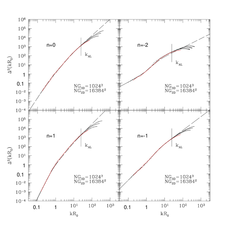
Figure 1: Comparison of the power spectrum measured from the 2D and 3D density fields. The data are the last three outputs of the simulations with the spectral index $n=1,0,-1,-2$. In each panel, the three short-dashed lines (middle) represent the 2D power spectrum measured from the last three outputs of the simulation, the solid line (bottom) is the 3D power spectrum measured from the last output of the simulation, and the long-dashed line (up) is the prediction by the fitting formula of Peacock & Dodds (1996). The value of $\rm NG$ represents the number of grid points adopted in their FFT respectively. We plot $\Delta^{2}(kR_{0})$ ($k=2\pi n/L,n=1,2\cdots$.) until $n=512$ for the 3D power spectrum, and until $n=3000$ for the 2D power spectrum. The wavenumber $k_{AL}$ at the vertical line is $k_{Ny}/3$ for 3D power spectrum. $R_{0}$ is the characteristic scale defined in Eq. (1).

In Figure 1 we compare the 2D power spectrum with the 3D power spectrum measured from the simulations with initial spectral index $1$, $0$, $-1$, and $-2$. The number of grid points of the 2D FFT is $16384^{2}$, and the number of the 3D FFT is $1024^{3}$. For the 3D power spectrum we plot $\Delta^{2}(kR_{0})$ ($k=nk_{b}$, $n=1,2\cdots$) for the last output of the simulations until $n=512$. As to the 2D case, we measured the power spectrum with the last three outputs of the simulations under the scaling transformation, and plot $\Delta^{2}(kR_{0})$ ( $k=2\pi n/L,n=1,2$ $\cdots$) until $n=3000$. Here we do not correct for the alias effect, and find that the alias begins to affect the power spectrum when the wavenumber is larger than $k_{AL}=k_{Ny}/3$ as indicated by the vertical lines in the picture. This picture also shows that the 2D power spectrum is identical to the 3D power spectrum when the alias effect is negligible.

In Figure 2 we compare the reduced bispectrum measured in the 2D and 3D density fields with the simulation of $n=-1$. We express the reduced bispectrum as a function of $k$, $v$ and $\theta$ as defined in Eq. (10). Each panel shows $Q(k,v,\theta)$ as a function of the angle $\theta$ between $\vec{k}_{1}$ and $\vec{k}_{2}$ with different $k$ and $v$. For the 3D bispectrum we only show the results of the last output for this simulation ($a=1$). For the 2D case we get the reduced bispectrum with the last two outputs of the simulation ($a=0.792,1$) under the scaling transformation. The corresponding $k$ values of the triangles are less than $k_{AL}$, so the alias does not affect the measured results. The figure shows that the bispectrum measured in 2D agrees very well with that in 3D, as expected.

From Figures 1 and 2, we conclude that it is reliable to use the 2D FFT instead of the 3D FFT to calculate the power spectrum and bispectrum on small scales. For the 2D particle distribution, an FFT with $N_{m}=8192$ requires computer memory about 0.3 Gbyte, even that with $N_{m}=16384$ requires memory about 1 Gbyte only. Therefore we can extend the bispectrum measurement into the strong nonlinear regime with little computer limitation.

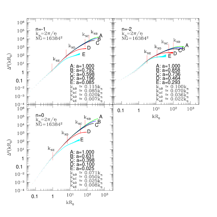
Figure 3: The power spectrum measured by FFT with the same number of grid points ($NG=16384^{2}$) for five epochs of the simulations, and scaled by the characteristic scale. These results are plotted by the lines A, B, C, D, E in each panel until $k_{AL}$, and their epochs are shown in the picture. The numerical artifacts begin to affect the power spectrum at the vertical line indicated by $k_{NB}$, $k_{NC}$, $k_{ND}$, $k_{NE}$ (in units of $k_{\eta}$, $\eta$ is the softening length), at which the deviation of the power spectrum from the true power spectrum is about 10 percent.

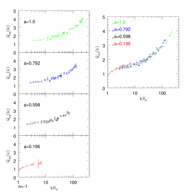
Figure 4: The reduced bispectrum for equilateral triangles measured by FFT with $NG_{2D}=8192^{2}$ or $NG_{3D}=1024^{3}$ for four epochs of the $n=-1$ simulation. The results are plotted up to the wavenumber at which the softening begins to influence the power spectrum (the vertical lines in Figure 3). Each panel on the left shows the results for one epoch. The points with and without error bars are measured from the 2D and 3D density fields respectively. We compare these results on the right panel where for clarity we do not show the errors.

In fact, $N_{m}=8192$ is sufficient to avoid the alias effect. In Figure 3, we show the power spectra at different epochs measured with the same number of FFT grid points. The deviation of the power spectrum from the scaling expectation at $k<k_{AL}$ should be attributed to the numerical artifacts in the simulations. From the figure, we find that these artifacts begin to influence the power spectrum at $k\approx 0.1k_{\eta}$ for late outputs where $k_{\eta}=2\pi/\eta$. We believe this is mainly caused by the force softening. For early outputs, the deviation from the scaling happens at a larger scale, which we attribute to the cutoff of the initial fluctuation at $k>k_{Ny}$ as well as the initial distribution of the particles on grid. All this shows that $N_{m}=8192$ is sufficient to explore the non-linear features in our simulations. In Figure  4 we check the softening effect on the reduced bispectrum. For simplicity we give the results only for spectral index $-1$. The left panels show the reduced bispectrum for equilateral triangles at four epochs up to the wavenumber where the softening begins to affect the power spectrum (as defined in Figure 3). The points with error bars are measured from the 2D density field, and those without error bars are obtained from the 3D density field. The error bars of the 2D bispectra are estimated from three projections. We compare these results on the right panel using the similarity scaling, which shows that the reduced bispectrum is not affected by the softening for the wavenumbers less than the softening limit set by the power spectrum analysis (Figure 3). We will use this criteria to minimize the softening effect in our $Q$ measurement.

We should point out that for a fixed range of $k$, the number of the Fourier modes is much smaller in 2D than in 3D. This limitation implies that the 2D FFT is not appropriate for the measurement at small wavenumbers. In our current analysis, we do both the 3D FFT with $N_{m}=1024$ and the 2D FFT with $N_{m}=8192$ for each simulation. For the wavenumber $k<2\pi/L\times 512/3$, we use $\delta(\vec{k})$ based on the 3D FFT; otherwise we use $\delta(\vec{k})$ based on the 2D FFT. For the 2D case, we have projected the density field along three axes. The 2D bispectrum is measured by averaging over the results of the three projections.

6 Results

6.1 Numerical results

In this section, we show the reduced bispectrum from the quasilinear regime to the strong non-linear regime measured with our new method. We have measured the bispectrum for many triangle shapes at different scales. In each case, we scale the results of two or three outputs with the characteristic scale defined by Eq. (1) in order to make sure that these results are not affected by numerical effects. For simplicity, in Figure 5 we show only a few measured bispectra for spectral index $1$, $0$, $-1$, $-2$, and these results scale very well. From the measured results (Figures  7, 9 and 11; left columns), we find that the results are in good agreement with the one-loop PT prediction in the quasilinear regime (Scoccimarro et al. 1998): the reduced bispectrum $Q$ is higher than the second-order PT for $n=-2$ and is smaller for $n\geq-1$. We also find that $Q$ depends on the triangle shape and size even in the strong nonlinear regime, which is in contrast with the hypothesis adopted by SF99 that $Q$ is a constant in this regime. It decreases with the initial spectral index and increases with the wavenumber, similar to what found for cold dark matter models (Jing & Börner 1998, Ma & Fry 2000, Scoccimarro, et al. 2001b, Takada & Jain 2003a).

6.2 A fitting formula for the bispectrum

SF99 presented a fitting formula for the bispectrum in scale-free clustering models. From Figures 7, 9 and 11 we find that the reduced bispectrum predicted by this formula agrees with the measured bispectrum at linear and quasilinear scales, and works well for some triangles with special shapes (such as $k_{1}=2k_{2}$ in the $n=-1$ model) in the strong nonlinear regime. But this formula cannot generally follow the bispectrum accurately at strongly nonlinear scales, because they assumed that the normalized bispectrum Q is a constant for a given initial spectral index, independent of the triangle’s wavenumber and shape. We provide a new fitting formula in this section to describe the nonlinear evolution of the bispectrum.

Hamilton et al. (1991) proposed a universal empirical relation between the linear $\xi_{L}$ and non-linear $\xi_{NL}$ two-point correlation functions. The relation is a powerful tool for predicting $\xi_{NL}$ in cosmological models. Later, Jain, Mo, & White (1995) demonstrated that the relation of Hamilton et al. fails for the scale-free model of $n=-2$. Peacock & Dodds (1996) examined a large set of scale-free models and CDM models, and obtained a accurate fitting formula for the power spectrum which agrees with the results of N-body simulations. Motivated by their work, we find that the ratio of the measured bispectrum to the weakly non-linear bispectrum (the second-order PT) has interesting properties, especially the behavior of $(Q_{nl}/Q_{l})^{1+0.25n}$ ($-2\leq n\leq 0$). A few typical examples of $(Q_{nl}/Q_{l})^{1+0.25n}$ are shown in Figures 6, 8 and 10 (the open symbols) for the three models with $n=0$, $-1$, and $-2$. From these results we expect that the relation between the weakly non-linear bispectrum and the nonlinear bispectrum can be expressed as:

$$Q_{nl}(kR_{0},v,\theta)=f_{nl}^{1/(1+0.25n)}\left(kR_{0},v,\theta,n)Q_{l}(kR_{0},v,\theta)\right),$$ (28)

where $n$ satisfies $-2\leq n\leq 0$. At linear scales $Q_{nl}\sim Q_{l}$, and $f_{nl}$ takes an asymptotic form as $f_{nl}(kR_{0},v,\theta,n)\sim 1$ in the linear regime. From the measured $(Q_{nl}/Q_{l})^{1+0.25n}$, we can find that $(Q_{nl}/Q_{l})^{1+0.25n}$ as a function of $\theta$ is approximated by a Gaussian function. Its difference from the Gaussian function is dependent on the triangle shape, scale and spectral index $n$. Taking into account of these factors, we propose the following form for $f_{nl}(kR_{0},v,\theta,n)$:

$$f_{nl}(kR_{0},v,\theta,n)={a_{1}(kR_{0},v,n)\exp\left(-\displaystyle{(\theta/\pi-a_{2}(kR_{0},v,n))^{2}\over a_{3}(kR_{0},v,n)}\right)+a_{4}(kR_{0},v,n)\over 1+a_{5}(kR_{0},v,n)(\theta/\pi)^{2}+a_{6}(kR_{0},v,n)(\theta/\pi)^{4}},$$ (29)

where $a_{i}(kR_{0},v,n)$ are:

$$a_{1}(kR_{0},v,n) = \{1-{2\over\exp(0.5(1-n)kR_{0})+1}+[(4+n)0.002v+$$

$$(0.012+0.008n)]kR_{0}\}[(0.1-0.3n)v+0.4],$$

$$a_{2}(kR_{0},v,n) = 0.5+0.2v,$$

$$a_{3}(kR_{0},v,n) = [1.-{2\over\exp(0.5kR_{0})+1}+(0.01nv+0.001)kR_{0}]0.04+$$

$$0.06v+0.1^{(1-n)},$$

$$a_{4}(kR_{0},v,n) = \{1.1+[(n^{2})^{1.3}0.05-0.2]\tanh(2kR_{0})+0.15\exp(-(0.3kR_{0})^{2})+$$

$$(0.01-{0.05-0.035v\over 4v+2})kR_{0}\}/[1+(0.4-0.2v)^{1+kR_{0}}],$$

$$a_{6}(kR_{0},v,n) = [0.8-{2\over\exp((0.5-n)kR_{0})+1}+(0.01-0.005/(v+0.1))kR_{0}]$$

$$[2-{0.3\over v+0.1}]+0.2n\tanh(2kR_{0}-1),$$

$$a_{5}(kR_{0},v,n) = -0.7a_{6}(kR_{0},v,n),$$ (30)

where $\tanh(x)=(\exp(x)-\exp(-x))/(\exp(x)+\exp(-x))$ is the hyperbolic function.

We have obtained the best-fitting parameters in $a_{i}(kR_{0},v,n)$ by doing a $\chi^{2}$ minimization between the predicted and measured bispectrum for all triangles. In Figures 6, 8 and 10 we compare the best fitting function $f_{nl}$ with our measured $(Q_{nl}/Q_{l})^{1+0.25n}$. The figures show that the fitting formula (29) works very well for $-2\leq n\leq 0$, for all triangle shapes, and for all scales (characterized by $kR_{0}$) studied. With the function $f_{nl}$, we can convert the weakly non-linear bispectrum into the non-linear bispectrum. In Figures 7, 9 and 11 we compare our measured reduced bispectra with the prediction of our fitting formula. There we also plot the prediction of the fitting formula of SF99. From the figures, one can see that the fitting formula obtained in this paper can accurately match the simulation results, much better than the formula of SF99.

To quantify the accuracy of our fitting formula, we plot the percentage of the deviation $\Delta Q/Q$ in Figures 12, 13 and 14. The deviation is defined as:

$${\Delta Q\over Q}={\mid Q_{fit}-Q_{simu}\mid\over Q_{simu}},$$ (31)

where $Q_{fit}$ is the prediction of our fitting formula, and $Q_{simu}$ is the reduced bispectrum measured from the simulations. Similarly we also estimate the accuracy of the fitting formula of SF99 that is also shown in the figures. The figures show that our fitting formula can match the measured results typically at an accuracy of 10 percent. The deviation is slightly larger, about $20\sim 30\%$, when $\theta\approx\pi$ and $kR_{0}<1$, which could be attributed to some stochastic fluctuation in $Q_{simu}$ for the limited number of k-triangles in the configuration. We also see that the deviation for the SF99 formula is much larger, almost about 50 percent in the strongly nonlinear regime.

Although we only have a single realization for these simulations, we measured the bispectrum for two or three outputs scaled according to the similarity solution. We regard each output as a realization, and estimate the errors of the bispectra from the different outputs. We also have taken the projections along different axes as independent realizations when we estimate errors for the 2D bispectra. In Figures 7, 9 and 11, the error bars are estimated with this method.

7 Summary and discussion

In this paper, we have accurately measured the bispectrum for four scale-free models. The measurement is based on a new method that can effectively eliminate the alias and numerical artifacts, and reliably extend the analysis into the strongly non-linear regime. The work also makes use of a set of state-of-the art N-body simulations of scale-free hierarchical models that have a significantly larger dynamical range than the previous studies. With these measured results, we demonstrated that the measured bispectrum depends on the shape and size of $k$-triangle even in the strongly nonlinear regime. It increases with wavenumber and decreases with the spectral index. These results are consistent with that those found for the three-point correlation for CDM models (Jing & Börner 1998, Ma & Fry 2000, Scoccimarro & Couchman 2001 , Scoccimarro et al. 2001b, Takada & Jain 2003a), but are in contrast with the hypothesis that $Q$ is a constant in the strongly non-linear regime (SF99). We also show that the fitting formula of SF99 does not describe our simulation results well, with a typical error about 40 percent. In the end, we present a new fitting formula for the reduced bispectrum that is valid for $-2\leq n\leq 0$ with a typical error of $10$ percent only.

Our new method for measuring the bispectra is to use the property that the 2D power spectrum and bispectrum are identical to the 3D ones. This property can be easily proved and has been tested with our N-body simulations. As the 2D FFT requires less computer memory than the 3D FFT, we can extend our analysis of the bispectrum into very small scales with little computer limitation. We also use the scaling properties of the scale-free models to correct for all known numerical artifacts and to identify those regimes where the bispectra can reliably measured.

Although we have obtained an empirical formula of the bispectrum for scale-free models of the spectral index $-2\leq n\leq 0$, some issues need to be addressed in future work. One obvious aspect is that the formula does not work for $n=1$, because the tree-level PT cannot predict the weakly non-linear bispectrum for this model. Fortunately the slope of the power spectrum in CDM models, which are the most plausible theory for the structure formation in the Universe, is in the range $-1$ to $-3$ at the non-linear scales. Therefore, we may generalize our fitting formula to CDM models by considering the change of the power spectrum slope with scale as well as the deviation from the Einstein-de Sitter model. We will study the bispectrum in CDM models in a future paper. Another issue is that our fitting formula is purely empirical. Considering that our measured $Q$ results are in good agreement with the one-loop PT prediction in the quasilinear regime (Scoccimarro et al. 1998) and that the halo model can successfully match the three-point correlation function in the strongly non-linear regime (Takada & Jain 2003a), we think it would be possible to combine these theoretical predictions to find a more theory-oriented fitting formula for $Q$.

     

     

Figure 2: Comparison of the reduced bispectrum measured from the 2D and the 3D density fields. The data are the last two outputs ($a=0.792$, $a=1.0$) of the simulation with spectral index $n=-1$. The solid line corresponds to the 3D reduced bispectrum at the last output of the simulation, and the open symbols are for the 2D reduced bispectrum at the last two outputs of the simulation under the scaling transformation. The left panels give $Q(k,v,\theta)$ for $kR_{0}=11.8$, and the right ones for $kR_{0}=17.8$.

     

     

     

Figure 5: The reduced bispectrum $Q(k,v,\theta)$ as a function of the angle $\theta$ between $\vec{k}_{1}$ and $\vec{k}_{2}$ for two or three outputs scaled by the characteristic scale. These results are measured by 3D FFT or 2D FFT as indicated at the bottom. The scales are also indicated. Different symbols (open circles, open triangles, open squares) stand for the results at different outputs.

     

Figure 6: The value of $(Q_{nl}/Q_{l})^{1/(1+0.25n)}$ as a function of $\theta$ for the spectral index $n=0$. $Q_{nl}$ is the reduced bispectrum measured from the simulation, and $Q_{l}$ is the weakly non-linear reduced bispectrum predicted by PT2. The solid line shows our fitting formula for $(Q_{nl}/Q_{l})^{1/(1+0.25n)}$, and the circle symbols are the simulation results. Vertical panel columns have the same $kR_{0}$, as indicated at the bottom.

     

Figure 7: The reduced bispectrum $Q(k,v,\theta)$ measured from the simulation with the spectral index $n=0$ (open circles), compared with the predictions by PT2 (long-dashed lines), by the fitting formula of SF99 (short-dashed lines), and by the fitting formula in this paper (solid lines). Vertical panel columns have the same $kR_{0}$, as indicated at the bottom.

     

Figure 8: Same as Fig.6, but for the spectral index $n=-1$.

     

Figure 9: Same as Fig.7, but for the spectral index $n=-1$.

     

Figure 10: Same as Fig.6, but for the spectral index $n=-2$.

     

Figure 11: Same as Fig.7, but for the spectral index $n=-2$.

     

Figure 12: The relative accuracy of the fitting formulae for the bispectrum for the spectral index $n=0$. The open circles are for the formula of SF99, and the solid lines are for the formula obtained in this paper.

     

Figure 13: Same as Fig.12, but for the spectral index $n=-1$.

     

Figure 14: Same as Fig.12, but for the spectral index $n=-2$.

simulation	$\eta/L$	timesteps	$a_{initial}$	$a_{firstoutput}$	$a_{final}$	outputs	$\Delta\log a_{i}$
n=1.	$1.\times 10^{-4}$	2000	0.0007	0.0042	1.0	10	0.266
n=0.	$1.\times 10^{-4}$	2000	0.0028	0.0157	1.0	10	0.20
n=$-1$	$1.\times 10^{-4}$	2000	0.0136	0.064	1.0	11	0.121
n=$-2$	$1.\times 10^{-4}$	2000	0.0834	0.2514	1.0	10	0.0667

Table 1: The scale-free simulations of $512^{3}$ particles

References

- Barriga & Gaztañaga (2002) Barriga, J. & Gaztañaga, E. 2002, MNRAS, 333, 443
- Bartelmann, & Schneider (2001) Bartelmann, M., & Schneider, P. 2001, Phys. Rep., 340, 291
- Baugh & Efstathiou (1994) Baugh, C. M. & Efstathiou, G. 1994, MNRAS, 270, 183
- Baugh, Gaztanaga, & Efstathiou (1995) Baugh, C. M., Gaztañaga, E., & Efstathiou, G. 1995, MNRAS, 274, 1049
- Bernardeau (1994) Bernardeau, F. 1994a, A&A, 291, 697
- Bernardeau, Singh, Banerjee, & Chitre (1994) Bernardeau, F., Singh, T. P., Banerjee, B., & Chitre, S. M. 1994b, MNRAS, 269, 947
- Bernardeau, Colombi, Gaztañaga, & Scoccimarro (2002) Bernardeau, F., Colombi, S., Gaztañaga, E., & Scoccimarro, R. 2002, Phys. Rep., 367, 1
- Bouchet, Colombi, Hivon, & Juszkiewicz (1995) Bouchet, F. R., Colombi, S., Hivon, E., & Juszkiewicz, R. 1995, A&A, 296, 575
- Colombi, Bouchet, & Hernquist (1996) Colombi, S., Bouchet, F. R., & Hernquist, L. 1996, ApJ, 465, 14
- Davis, Efstathiou, Frenk, & White (1985) Davis, M., Efstathiou, G., Frenk, C. S., & White, S. D. M. 1985, ApJ, 292, 371
- Efstathiou, Davis, White, & Frenk (1985) Efstathiou, G., Davis, M., White, S. D. M., & Frenk, C. S. 1985, ApJS, 57, 241
- Efstathiou, Frenk, White, & Davis (1988) Efstathiou, G., Frenk, C. S., White, S. D. M., & Davis, M. 1988, MNRAS, 235, 715
- Frieman & Gaztañaga (1999) Frieman, J. A. & Gaztañaga, E. 1999, ApJ, 521, L83
- Fry (1984) Fry, J. N. 1984, ApJ, 279, 499
- Fry & Gaztanaga (1993) Fry, J. N. & Gaztañaga, E. 1993, ApJ, 413, 447
- Fry (1994) Fry, J. N. 1994, Physical Review Letters, 73, 215
- Fry, Melott, & Shandarin (1995) Fry, J. N., Melott, A. L., & Shandarin, S. F. 1995, MNRAS, 274, 745
- Gaztañaga & Frieman (1994) Gaztañaga, E. & Frieman, J. A. 1994, ApJ, 437, L13
- Gaztanaga & Baugh (1995) Gaztañaga, E. & Baugh, C. M. 1995, MNRAS, 273, L1
- Hamilton, Matthews, Kumar, & Lu (1991) Hamilton, A. J. S., Matthews, A., Kumar, P., & Lu, E. 1991, ApJ, 374, L1
- Hamana et al. (2002) Hamana, T., Colombi, S. T., Thion, A., Devriendt, J. E. G. T., Mellier, Y., & Bernardeau, F. 2002, MNRAS, 330, 365
- Hivon, Bouchet, Colombi, & Juszkiewicz (1995) Hivon, E., Bouchet, F. R., Colombi, S., & Juszkiewicz, R. 1995, A&A, 298, 643
- Hockney & Eastwood (1981) Hockney, R. W. & Eastwood, J. W. 1981, Computer Simulation Using Particles, New York: McGraw-Hill, 1981
- Jain, Mo, & White (1995) Jain, B., Mo, H. J., & White, S. D. M. 1995, MNRAS, 276, L25
- Jain & Bertschinger (1998) Jain, B. & Bertschinger, E. 1998, ApJ, 509, 517
- Jing (1992) Jing, Y. P. 1992, Ph.D. Thesis
- Jing (2004) Jing, Y. P. 2004, astroph/0409240
- Jing, Borner, & Valdarnini (1995) Jing, Y. P., Börner, G., & Valdarnini, R. 1995, MNRAS, 277, 630
- Jing (1998) Jing, Y. P. 1998, ApJ, 503, L9
- Jing & Boerner (1997) Jing, Y. P. & Börner, G. 1997, A&A, 318, 667
- Jing & Boerner (1998) Jing, Y. P. & Börner, G. 1998, ApJ, 503, 37
- Jing & Suto (2002) Jing, Y. P. & Suto, Y. 2002, ApJ, 574, 538
- Jing & Boerner (2004) Jing, Y. P. & Börner, G. 2004, ApJ, 607, 140
- Juszkiewicz, Bouchet, & Colombi (1993) Juszkiewicz, R., Bouchet, F. R., & Colombi, S. 1993, ApJ, 412, L9
- Lokas, Juszkiewicz, Weinberg, & Bouchet (1995) Łokas, E. L., Juszkiewicz, R., Weinberg, D. H., & Bouchet, F. R. 1995, MNRAS, 274, 730
- Issha Kayo et al. (2004) Kayo, I., et al., 2004, preprint (astro-ph/0403638)
- Ma & Fry (2000) Ma, C. & Fry, J. N. 2000, ApJ, 538, L107
- Matarrese, Verde, & Heavens (1997) Matarrese, S., Verde, L., & Heavens, A. F. 1997, MNRAS, 290, 651
- Mo, Jing, & White (1997) Mo, H. J., Jing, Y. P., & White, S. D. M. 1997, MNRAS, 284, 189
- Peacock & Dodds (1996) Peacock, J. A. & Dodds, S. J. 1996, MNRAS, 280, L19
- Peebles (1980) Peebles, P. J. E., 1980, The Large-Scale Structure of the Universe. Princeton Univ. Press, Princeton NJ
- Pen et al. (2003) Pen, U., Zhang, T., van Waerbeke, L., Mellier, Y., Zhang, P., & Dubinski, J. 2003, ApJ, 592, 664
- Schneider et al. (2003) Schneider, P., Kilbinger, M. , & Lombardi, M., preprint (astro-ph/0308328)
- Scoccimarro & Frieman (1996) Scoccimarro, R. & Frieman, J. A. 1996, ApJ, 473, 620
- Scoccimarro (1997) Scoccimarro, R. 1997, ApJ, 487, 1
- Scoccimarro et al. (1998) Scoccimarro, R., Colombi, S., Fry, J. N., Frieman, J. A., Hivon, E., & Melott, A. 1998, ApJ, 496, 586
- Scoccimarro & Frieman (1999) Scoccimarro, R. & Frieman, J. A. 1999, ApJ, 520, 35
- Scoccimarro & Couchman (2001) Scoccimarro, R. & Couchman, H. M. P. 2001, MNRAS, 325, 1312
- Scoccimarro, Sheth, Hui, & Jain (2001) Scoccimarro, R., Sheth, R. K., Hui, L., & Jain, B. 2001b, ApJ, 546, 20
- Scoccimarro, Feldman, Fry, & Frieman (2001) Scoccimarro, R., Feldman, H. A., Fry, J. N., & Frieman, J. A. 2001c, ApJ, 546, 652
- Simth et al. (2003) Smith, R.E., Peacock, J. A., Jenkins, A., White, S. D. M., Frenk, C. S., Pearce, F. R., P.A. Thomas, P. A., Efstathiou, G., Couchmann, H. M. P. 2003, MNRAS, 341, 1311
- Takada & Jain (2003) Takada, M. & Jain, B. 2003a, MNRAS, 340, 580
- Takada & Jain (2003) Takada, M. & Jain, B. 2003b, MNRAS, 344, 857
- Verde, Heavens, Matarrese, & Moscardini (1998) Verde, L., Heavens, A. F., Matarrese, S., & Moscardini, L. 1998, MNRAS, 300, 747
- Verde et al. (2002) Verde, L., et al. 2002, MNRAS, 335, 432
- Van Waerbeke et al. (2001) Van Waerbeke L., Hamana T., Scoccimarro R.,Colombi S., Bernardeau F., 2001, MNRAS, 322, 918
- wang et al. (2004) Wang,Y., Yang, X., Mo, H. J., van den Bosch, F. C., Chu, Y.Q., preprint (astro-ph/0404143)
- Zhang, Pen, Zhang, & Dubinski (2003) Zhang, T., Pen, U., Zhang, P., & Dubinski, J. 2003, ApJ, 598, 818