Helical coronal ejections and their role in the solar cycle

Abstract

The standard theory of the solar cycle in terms of an alpha-Omega dynamo hinges on a proper understanding of the nonlinear alpha effect. Boundary conditions play a surprisingly important role in determining the magnitude of alpha. For closed boundaries, the total magnetic helicity is conserved, and since the alpha effect produces magnetic helicity of one sign in the large scale field, it must simultaneously produce magnetic helicity of the opposite sign. It is this secondary magnetic helicity that suppresses the dynamo in a potentially catastrophic fashion. Open boundaries allow magnetic helicity to be lost. Simulations are presented that allow an estimate of alpha in the presence of open or closed boundaries, either with or without solar-like differential rotation. In all cases the sign of the magnetic helicity agrees with that observed at the solar surface (negative in the north, positive in the south), where significant amounts of magnetic helicity can be ejected via coronal mass ejections. It is shown that open boundaries tend to alleviate catastrophic alpha quenching. The importance of looking at current helicity instead of magnetic helicity is emphasized and the conceptual advantages are discussed.

1 Introduction

The emerging magnetic field of the sun frequently displays strong signs of twist. The systematic investigation of twist began with the early work of [Seehafer (1990)] who analyzed the current helicity in active regions and found a hemispheric dependence of its sign: negative in the north, positive in the south. This dependence has since been confirmed and the statistics improved. The investigation of helicity is usually motivated by the interest in a detailed description of the degree of complexity of the solar magnetic field. There has also been some interest in understanding the reasons for the observed twist (or helicity). In recent years, however, a very different question has emerged: how is it possible that the solar dynamo works as it does? Given that in simulations the value of the Spitzer resistivity still affects the cycle period ([Brandenburg et al. 2002]), one would like to understand how this is avoided in a proper theory of the solar cycle.

The significance of this question is often not very evident, but this is mainly because in many simulations the values of the magnetic Reynolds number are still not large enough. It should be emphasized that the involvement of the microscopic diffusivity in the description of macroscopic properties of a turbulent flow is a highly unusual property of MHD that is not normally encountered anywhere else in turbulence.

What is so special here is that the magnetic helicity is an almost perfectly conserved quantity. This can have serious implications for the operation of the large scale dynamo effect in the nonlinear regime. An example where this is true is the $\alpha$ effect in mean field electrodynamics ([Moffatt 1978]; [Krause & Rädler 1980]). As more and more large scale field is produced by the $\alpha$ effect, and since the large scale field produced by the $\alpha$ effect is helical (with a sign equal to that of $\alpha$), there must be a simultaneous generation of magnetic helicity of the opposite sign such that the total magnetic helicity is conserved. (What actually matters for the $\alpha$ effect is the current helicity, not the magnetic helicity, but the two are related.)

The quenching of $\alpha$ can also affect the quenching of the turbulent magnetic diffusivity and this in turn the cycle period. Even though the cycle period of 22 years is significantly longer than the local turnover time of the turbulence, we do not necessarily expect the cycle period to depend on the magnetic diffusion time. As pointed out earlier ([Brandenburg et al. 2002]), the idea of the cycle period being dependent on the magnetic diffusion time is not completely unrealistic: The magnetic helicity constraint dictates that the change $\Delta H_{\rm N}$ of the magnetic helicity during the solar cycle, normalized by the magnetic energy $M_{\rm N}$, where the subscript N refers to the northern hemisphere, must not exceed the skin depth if the change in magnetic helicity is brought about by purely resistive effects (the same applies separately for the southern hemisphere). Models of the solar dynamo suggest that the ratio $\Delta H_{\rm N}/(2\mu_{0}M_{\rm N})$ is about $70\,{\rm km}$. In the sun the skin depth based on the cycle period varies between $10\,{\rm km}$ at the bottom of the convection zone and $300\,{\rm km}$ at the top. Thus, unless the dynamo works only in a thin surface layer, $\Delta H_{\rm N}$ is too large compared to the $10\,{\rm km}$ figure. Therefore one might hope that open boundaries can alleviate this constraint, although the effect does not need to be very strong.

The effect of open boundaries has already been investigated in the past in a model without differential rotation ([Brandenburg & Dobler 2001]). It was found that open boundaries do lead to the expected reduction of the saturation time scale, but the amplitude of the final field strength was also reduced dramatically. In the following we report on recent simulations of [Brandenburg & Sandin] (2004, hereafter referred to as BS), where the effect of open boundaries has been investigated in a model with solar-like differential rotation. This was found to lead to an increase of the saturation field strength by a factor of about 30. Such an increase was associated with the effect of a current helicity flux. In the following we discuss their model in more detail and present new calculations of the resulting dynamo action.

2 A cartesian model of the solar differential rotation

In order to model the region below $30^{\circ}$ latitude, BS have adopted a cartesian geometry where the $x$ direction corresponds to radius, the $y$ direction to longitude, and the $z$ direction to latitude. The mean toroidal velocity is given by

$$\overline{\mbox{\boldmath$U$}}=U_{0}\cos k_{1}x\cos k_{1}z,$$ (1)

where $k_{1}$ is the lowest wavenumber in the $(x,z)$ plane with $-\pi/2\leq k_{1}x\leq 0$ and $0\leq k_{1}z\leq\pi/2$. In the following we adopt units where $k_{1}=1$. The equator is assumed to be at $z=0$ and the outer surface at $x=0$. The bottom of the convection zone is at $x=-\pi/2$ and the latitude where the surface angular velocity equals the value in the radiative interior is at $z=\pi/2$; see figure 1.

Figure 1: On the left hand side a sketch of the solar angular velocity at low latitudes is shown, with spoke-like contours in the bulk of the convection zone merging gradually into uniform rotation in the radiative interior. The low latitude region, considered in this paper, is indicated by thick lines. On the right hand side we show the differential rotation as modeled in our cartesian box. The equator corresponds to the bottom, the surface to the right, the bottom of the convection zone to the left and mid-latitudes at the top of the box. The boundary conditions for the three components of the magnetic field and the vector potential are indicated near the boundaries of the box.

In order to test the properties of this differential rotation, BS investigated first the resulting dynamo action in a mean field model. This should give some idea of the type of solutions that one might expect in a three-dimensional model where helical turbulence is able to sustain dynamo action without explicitly invoking an $\alpha$ effect.

In figure 2 we plot the stability diagram in the $(C_{\alpha},C_{S})$ plane, where $C_{\alpha}=\alpha/\eta_{\rm T}k_{1}$ and $C_{S}=U_{0}/\eta_{\rm T}k_{1}$ are nondimensional measures of $\alpha$ effect and shear. For $C_{\alpha}<C_{\alpha,{\rm crit}}$ the solutions are decaying and for $C_{\alpha}>C_{\alpha,{\rm crit}}$ they are growing exponentially and are oscillatory (Hopf bifurcation), except for a narrow interval around $C_{S}=0$. Such a behavior is quite typical of $\alpha\Omega$ dynamos (see, e.g., [Roberts & Stix 1972]). For $C_{S}=1000$ we have also considered the quadrupolar solution by changing the boundary condition on the equator in the appropriate way. It turns out that it is slightly easier to excite (see figure 2). As stated earlier, the approximately equal excitation conditions for dipolar and quadrupolar solutions, seen in figure 2, are typical of $\alpha\Omega$ dynamos in spherical shells. Indeed, the fact that quadrupolar solutions can be preferred has been found in other solar dynamo models ([Dikpati & Gilman 2001]).

Figure 2: Critical value of $C_{\alpha}$ for dynamo action as a function of shear parameter, $C_{S}$. Note the typical decrease of the critical value of $C_{\alpha}$ with increasing $C_{S}$. The dash-dotted line corresponds to the parameter regime of the turbulence simulations discussed below.

We may conclude that the present cartesian setup provides a useful representation of a global model of the sun’s differential rotation. The mean field model reproduces similar features to those found in global mean field models in spherical shells.

3 Results for $\alpha$ quenching

Next, BS focussed on the investigation of helicity-driven turbulence in the presence of shear as given by eq. (1). Instead of looking for dynamo action, they considered the case of an imposed magnetic field in the $y$ direction of strength $B_{0y}$. They determined $\alpha$ by measuring the turbulent electromotive force, i.e. $\alpha=\langle\mbox{\boldmath${\cal E}$}{}\rangle\cdot\mbox{\boldmath$B$}{}_{0}/B_{0}^{2}$. They presented a range of simulations for different values of the magnetic Reynolds number,

$$R_{\rm m}=u_{\rm rms}/(\eta k_{\rm f}),$$ (2)

for both open and closed boundary conditions. (Here, $u_{\rm rms}$ does not include the mean shear flow.) In the simulations, $U_{0}/u_{\rm rms}\approx 10$ and $\alpha/u_{\rm rms}\approx 0.1$ (figure 3). Using $\eta_{\rm T}=c_{\eta}u_{\rm rms}/k_{\rm f}$, where $c_{\eta}$ is a free parameter, we have $C_{S}/C_{\alpha}\approx 100$, which is marked in figure 2 as a dash-dotted line. The intersection with the sequence of points from the mean field calculation gives $C_{S}\approx 150$, and since

$$C_{S}\equiv{U_{0}\over\eta_{\rm T}k_{1}}\approx{U_{0}k_{\rm f}\over c_{\eta}u_{\rm rms}k_{1}}\approx{50\over c_{\eta}}$$ (3)

and $k_{\rm f}/k_{1}=5$ we find $c_{\eta}\approx 0.3$. This value appears reasonable, although somewhat smaller that the value of 0.8 obtained from magnetic decay experiments ([Yousef et al. 2003]). The value of $C_{S}\approx 150$ suggests that our simulations should be in an oscillatory regime, which is indeed confirmed (see § 4).

There is a striking difference between the cases with open and closed boundaries which becomes particularly clear when comparing the averaged values of $\alpha$ for different magnetic Reynolds numbers; see figure 3. With closed boundaries $\alpha$ tends to zero like $R_{\rm m}^{-1}$, while with open boundaries $\alpha$ shows no such immediate decline; only for larger values of $R_{\rm m}$ there is possibly an asymptotic $\alpha\propto R_{\rm m}^{-1}$ dependence. There is also a clear difference between the cases with and without shear. In the absence of shear (dotted line in figure 3) $\alpha$ declines with increasing $R_{\rm m}$, even though for small values of $R_{\rm m}$ it is larger than with shear. This suggests that the presence of shear combined with open boundaries might be a crucial prerequisite of dynamos that saturate on a dynamical time scale.

Figure 3: Dependence of $|\langle\alpha\rangle|/u_{\rm rms}$ on $R_{\rm m}$ for open and closed boundaries. The case with open boundaries and negative helicity is shown as a dashed line. Note that for $R_{\rm m}\approx 30$ the $\alpha$ effect is about 30 times smaller when the boundaries are closed. The dotted line gives the result with open boundaries but no shear. The vertical lines indicate the range obtained by calculating $\alpha$ using only the first and second half of the time interval.

The difference between open and closed boundaries can be explained in terms of a current helicity flux through the two open open boundaries of the domain. Instead of going through the mathematical formalism, we just present the argument in words. First of all, in the kinematic regime (i.e. for weak fields) the $\alpha$ effect is a negative multiple of the kinetic helicity. As the magnetic field grows, there will also be a growing small scale magnetic field which itself is helical and it too enters in the calculation of $\alpha$. The relevant quantity is the mean current helicity of the small scale, $\overline{\mbox{\boldmath$j$}{}\cdot\mbox{\boldmath$b$}{}}$. Its sign is that of the kinetic helicity, i.e. negative in the northern hemisphere, and it enters with a minus sign, so it acts in such a way as to quench the total $\alpha$ effect ([Pouquet et al. 1976]). The next important step is to find the evolution equation for $\overline{\mbox{\boldmath$j$}{}\cdot\mbox{\boldmath$b$}{}}$ in terms of the mean field. This can be done in the same way as in the calculation of the kinematic $\alpha$ effect, e.g. by using the first order smoothing approach, or by other techniques (see [Brandenburg & Subramanian (2004), Brandenburg & Subramanian 2004] for a review). It is simpler, however, to use magnetic helicity conservation, so one has to convert from current helicity, $\overline{\mbox{\boldmath$j$}{}\cdot\mbox{\boldmath$b$}{}}$, to magnetic helicity, $\overline{\mbox{\boldmath$a$}{}\cdot\mbox{\boldmath$b$}{}}$. Under isotropic conditions we have $\overline{\mbox{\boldmath$j$}{}\cdot\mbox{\boldmath$b$}{}}=k_{\rm f}^{2}\,\overline{\mbox{\boldmath$a$}{}\cdot\mbox{\boldmath$b$}{}}$, where $k_{\rm f}$ is the wavenumber of the fluctuating (small scale) field. The time dependence of the magnetic helicity equation cannot usually be ignored. It is important to explain the slow saturation behavior found in helical dynamos in closed and periodic boxes. But after a resistive time scale (which can be very long) the time dependence can be ignored. In that case the magnetic helicity equation says that the production of small scale magnetic helicity (which is equal and opposite in sign to the production of large scale magnetic helicity and hence large scale magnetic field) must be balanced by the magnetic helicity dissipation term (i.e. the current helicity times the resistivity). The latter term is hence resistively small, which is why the electromotive force, and hence the $\alpha$ effect, are catastrophically quenched. However, when there are open boundary conditions, the situation changes and the electromotive force can now be balanced by the divergence of the current helicity flux. The fact that even for the open boundary conditions the curves tend to bend downward might suggest that the current helicity flux term itself could depend on the small scale magnetic diffusivity. If this turns out to be the case, it may indicate that the vertical field boundary conditions used here do not represent a sufficiently realistic representation of the solar surface conditions.

Figure 4: Normal components of the current helicity flux on the outer surface ($\overline{\cal F}_{x}$) and at the equator ($\overline{\cal F}_{z}$), averaged over the corresponding surfaces. The fat lines denote the fluxes from the small scale field, $\overline{\mbox{\boldmath${\cal F}$}}{}_{C}^{\rm SS}$, while the thin lines denote the fluxes form the large scale field, $\overline{\mbox{\boldmath${\cal F}$}}{}_{C}^{\rm LS}$. The dotted lines near the two $\overline{\mbox{\boldmath${\cal F}$}}{}_{C}^{\rm LS}$ curves show the result of the approximation $\overline{\mbox{\boldmath${\cal F}$}}{}_{C}^{\rm LS}\approx-2(\overline{J}_{y}\overline{U}_{y})\overline{\mbox{\boldmath$B$}}$.

In figure 4 we also show the small scale current helicity fluxes on the two boundaries (fat lines). There is a tendency for the difference between incoming flux at the equator (fat dotted line) and outgoing fluxes at outer surface (fat solid line) to cancel, but the net outgoing flux is again negative.

A full investigation of the magnetic and current helicity losses associated with dynamo action may really require global models in spherical geometry. However, some preliminary information can already now be gained by studying local models with imposed solar-like differential rotation. In mean field models such a geometry reproduces many of the features that are known from corresponding mean field models in full spherical geometry.

Models with helically driven turbulence and an imposed toroidal magnetic field allow the determination of the $\alpha$ effect. It turns out that the catastrophic quenching of the $\alpha$ effect is alleviated (at least by a factor of about 30) when magnetic and current helicity is allowed to leave the domain. The simulations have shown that a reasonable estimate for the current helicity flux at the outer surface is

$$\overline{\mbox{\boldmath${\cal F}$}}{}_{C}\approx 30\,u_{\rm rms}k_{\rm f}B_{0}^{2}.$$ (4)

Applying this to the sun using $u_{\rm rms}\approx 50\,{\rm m/s}$ for the rms velocity in the deeper parts of the convection zone, $k_{\rm f}\approx 10^{-9}\,{\rm cm}^{-1}$ based on the inverse mixing length, and $B_{0}\approx 3\,{\rm G}$ for the mean field at the solar surface, we have $\overline{\mbox{\boldmath${\cal F}$}}{}_{C}\approx 10^{-3}\,\,{\rm G^{2}\!/s}$. The current helicity flux integrated over the northern hemisphere of the sun is then $4\times 10^{19}\,{\rm G}^{2}\,{\rm cm}^{2}\,{\rm s}^{-1}$. Integrated over the 11 yr solar cycle we have $10^{28}\,{\rm G}^{2}\,{\rm cm}^{2}$.

Figure 5: Sketch illustrating the directions of large scale (LS) and small scale (SS) negative current helicity fluxes and their approximate magnitudes (in units of $\overline{\mbox{\boldmath${\cal F}$}}{}_{0}$). Note that at the outer surface negative current helicity is ejected both via small and large scale fields, while at the equator the contributions from small and large scale fields have opposite sign. The small scale losses at surface and equator partially cancel, giving a net loss of negative current helicity of only about $4\,\overline{\mbox{\boldmath${\cal F}$}}{}_{0}$.

For the sun only magnetic helicity fluxes have been determined. As a rough estimate we may use $\overline{\mbox{\boldmath${\cal F}$}}{}_{H}\approx k_{\rm f}^{-2}\overline{\mbox{\boldmath${\cal F}$}}{}_{C}$ for the magnetic helicity flux. Using the same estimate for $k_{\rm f}$ as above we obtain about $10^{46}\,{\rm Mx}^{2}$ over the 11 yr solar cycle. This is indeed comparable to the magnetic helicity fluxes estimated by [Berger & Ruzmaikin (2000)] and [DeVore (2000)].

4 Three-dimensional dynamo action

In order to study the full dynamo operation we now present simulations without imposed field. In figure 6 we show an example of such a simulation where, in addition to the helically driven turbulence (with negative helicity), an outer coronal buffer layer has been added to allow the magnetic field to be expelled from the turbulent dynamo zone.

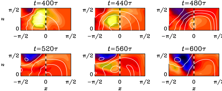
Figure 6: The toroidally averaged field from a simulation without imposed field. Poloidal field lines are superimposed on a color/grey scale representation of the mean toroidal field. The coronal buffer layer is to the right of the dashed line. The frames are separated by about 40 turnover times, i.e. $\Delta t/(u_{\rm rms}k_{\rm f})=40$. Note the migration of magnetic field toward the surface.

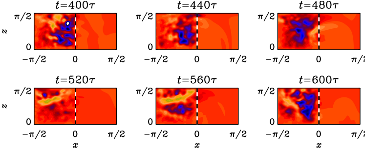
Figure 7: Gray/color scale plot of the total current helicity density, $\overline{\mbox{\boldmath$J$}}\cdot\overline{\mbox{\boldmath$B$}}+\overline{\mbox{\boldmath$j$}{}\cdot\mbox{\boldmath$b$}{}}$ in the meridional plane. Dark/blue represents negative values, and intermediate/red shades indicate zero. The coronal buffer layer is to the right of the dashed line. Note that the total current helicity density is mostly negative, but it’s magnitude tends to be smaller near the boundaries.

These studies are still preliminary and need to be carried out for a range of different magnetic Reynolds numbers before we are able to tell whether the open boundaries are really able to alleviate the catastrophic $\alpha$ quenching that occurs in the presence of closed or periodic boundaries; see Table 5 of [Brandenburg et al. 2002, Brandenburg et al. (2002)]. Nevertheless, a few interesting aspects can already be recognized. Firstly, there is some migration-like evolution of the toroidally averaged magnetic field in the meridional plane – similar to what is expected from the mean field model (BS). Secondly, by looking at the toroidally averaged current helicity (mean and fluctuating parts together), one sees mostly negative values (corresponding to dark shades in figure 7). On the open boundaries the current helicity is close to zero. Only near the outer surface there is occasionally a dominance of negative values.

5 Conclusions

Finally, in the absence of an imposed toroidal field a large scale magnetic field is generated that shows features of field migration toward the surface, similar to what the mean field shows. More work is obviously required to test the dependence of the cycle period on the magnetic Reynolds number. Also, it would be interesting to allow for a (nearly) force-free coronal magnetic field that permits a more direct connection between the helicity losses and the field geometry associated with these losses. Ideally, of course, one would like to model proper coronal mass ejections in the context of this model.