XMM-Newton Observations of A133: A Weak Shock Passing through the Cool Core

Abstract

We use XMM-Newton observations of the cluster of galaxies A133 to study the X-ray spectrum of the intracluster medium (ICM). We find a cold front to the southeast of the cluster core. From the pressure profile near the cold front, we derive an upper limit to the velocity of the core relative to the rest of the cluster of $<230$ km s^-1. Our previous Chandra image of A133 showed a complex, bird-like morphology in the cluster core. Based on the XMM-Newton spectra and hardness ratio maps, we argue that the wings of this structure are a weak shock front. The shock was probably formed outside the core of the cluster, and may be heating the cluster core. Our Chandra image also showed a “tongue” of relatively cool gas extending from the center of the cD to the center of the radio relic. The XMM-Newton results are consistent with the idea that the tongue is the gas which has been uplifted by a buoyant radio bubble including the radio relic to the northwest of the core. Alternatively, the tongue might result from a cluster merger. The small velocity of the core suggests that the bubble including the relic has moved by buoyancy, rather than by motions of the core or the ICM. We do not find clear evidence for nonthermal X-ray emission from the radio relic. Based on the upper limit on the inverse Compton emission, we derive a lower limit on the magnetic field in the relic of $B\geq 1.5$ $\mu$G.

1 Introduction

A133 is an X-ray luminous cluster at $z=0.0562$ (Way, Quintana, & Infante, 1997). The cluster shows substructure which may indicate that it is undergoing a merger (Krywult, MacGillivray, & Flin, 1999). However, it was said that there is a moderate cooling flow at the center of the cluster ($\dot{M}=110\,M_{\sun}\>\rm yr^{-1}$ for $H_{0}=50\>\rm km\>s^{-1}\>Mpc^{-1}$; White, Jones, & Forman, 1997). The central cD galaxy is a radio source. About 30^′′ north of the cD galaxy, there is a diffuse radio relic source, which has a “spidery” filamentary structure and an extremely steep spectral index (Slee et al., 2001). ROSAT observations suggested that there might be excess X-ray emission associated with the radio relic (Slee et al., 2001; Rizza et al., 2000).

Fujita et al. (2002) observed A133 with Chandra and showed that the central cool core is irregular; the dominant feature is a “tongue” of cool X-ray gas which extends to the northwest of the cD galaxy. The tongue ends on and overlaps the radio relic, at least in projection. Excluding the tongue, the X-ray surface brightness at the relic is about 30% fainter than the surrounding region. There is no clear evidence for a merger shock near the radio relic, at least in the Chandra image. On the other hand, the Chandra spectrum gave a (at best) marginal detection of inverse Compton emission. The position of the cD galaxy coincides with the brightest X-ray emission, but is shifted to the southeast of the X-ray centroid determined on larger scales in the cluster.

Fujita et al. (2002) discussed several possible origins for the tongue; two of these seem reasonably consistent with the X-ray and radio data. First, the tongue may be the result of a Kelvin-Helmholtz instability acting on the cool core surrounding the cD galaxy as the cD galaxy moves through surrounding, lower density gas. The second possibility is that the radio relic is a buoyant radio bubble and that the tongue was uplifted by the motion of this bubble, as appears to have occurred in M87/Virgo. In order to constrain these models further, detailed spectral information is needed.

In this paper, we report the XMM-Newton observations of A133. XMM-Newton has a larger field of view and much more collecting area at high energies than Chandra. Combining these rich spectral data with the existing Chandra images, we discuss the origin of the complicated central structures of A133. We assume $H_{0}=70\>\rm km\>s^{-1}\>Mpc^{-1}$, $\Omega_{0}=0.3$, and $\Lambda=0.7$ unless otherwise noted. At a redshift of 0.0562, $1\arcsec$ corresponds to 1.07 kpc.

2 XMM-Newton Observation and Data Analysis

A133 was observed with XMM-Newton (Jansen et al., 2001) on 2002 December 22–23 for a total exposure time of 33.7 ks. The EPIC-MOS cameras were operated in Full Frame mode and the EPIC-PN camera in Extended Full Frame mode (Turner et al., 2001; Strüder et al., 2001). The Thin filter was used in all EPIC observations. We created calibrated event files using SAS Version 5.4.1, and all further reduction and analysis used this version of SAS.

Data obtained with XMM-Newton are often affected by periods of high background flares, which need to be removed. We adopted the cleaning method described in detail in Reiprich et al. (2004). In order to determine lightcurves free from the contamination from astrophysical sources, we chose the energy band of $10$–$12$ keV and $12$–$14$ keV for the MOS and PN cameras, respectively. The exposure time was binned in 100 s intervals and only events with pattern $\leq 12$ and $\sharp$XMMEA_EM (MOS) or flag $=0$ (PN) were used. We applied conservative ‘generic’ cuts to the count rates $C_{X}$ before we estimated the mean count rates to find background flares. For MOS (PN), only times with $0.01\>(0.02)\leq C_{X}\leq 0.25\>(0.45)$ counts per second have been used. Finally, we obtained the good time intervals (GTIs) by including only times where the count rates are within $\pm 2\sigma$ of the mean count rates. The final count-rate ranges are $0.03$–$0.17$ (MOS1), $0.02$–$0.18$ (MOS2), and $0.09$–$0.30$ (PN) counts per second. The useful exposure times after these procedures are 20.9 ks (MOS1 and MOS2) and 15.4 ks (PN).

After the flaring background is removed, we further need to remove the quiet background. Since the emission from the cluster covers most of the fields of view of the detectors, we used the quiet background created from blank sky observations. These background files have been screened for high flaring background periods and background spectra have been extracted with the same selection criteria as the source spectra. We found source-to-background count-rate ratios of 1.10 for MOS1, 1.09 for MOS2, and 1.17 for the PN detector and rescaled the background files by rewriting the BACKSCAL header keyword according to these values. We note that the results are not much affected by quiet background, because we mostly focus on the bright central region of the cluster.

Figure 1a shows the combined MOS1-MOS2-PN image of A133 in the $0.3$–$2$ keV energy band; this band was used to emphasize the complicated central structure of the cluster, which is mainly due to gas being cooler and thus more prominent at low energies. The image is corrected for background, exposure, and vignetting, and was adaptively smoothed to a minimum signal-to-noise ratio of 15 per smoothing beam. For comparison, in Figure 1b we also present the central $2\arcmin\times 2\arcmin$ image obtained with Chandra (Fig. 1b in Fujita et al., 2002). Figure 2 shows the hardness ratio map of A133. We define the hardness ratio as the combined MOS1-MOS2-PN count rate in the $2$–$10$ keV band divided by the count rate in the $0.3$–$2$ keV band. The central region and the tongue are cold. There is a temperature jump at the southeast edge of the cool core, which will be discussed in § 3.1 and 4.1.

3 Spectral Analysis

We extracted spectra in the $0.5$–$10$ keV (MOS) and $0.3$–$12$ keV (PN) bands from selected regions of the XMM-Newton image using the SAS software package. Only single and double events were used to extract PN spectra. The response matrices we used were m11_r7_im_all_2002-11-07.rmf for MOS1, m21_r7_im_all_2002-11-07.rmf for MOS2, and epn_ef20_sdY9.rmf for PN. The ancillary response files were calculated using arfgen (Version 1.48.8). The spectra were grouped to have a minimum of 50 counts per bin and fitted with spectral models using XSPEC, Version 11.2. All errors are quoted at the 90% confidence level unless otherwise mentioned. Spectra obtained with MOS1 and MOS2 were fitted simultaneously; fitting MOS1 and MOS2 separately gives consistent results.

3.1 Projected Profiles

Figures 3 and 4 show the radial profiles of projected temperature and abundance for four sectors, respectively. We define the projected temperature (projected abundance) to be the X-ray emission-weighted temperature (abundance) along the line of sight. Spectra obtained with MOS1 and MOS2 were simultaneously fitted. The position angles (north through east) are $0^{\circ}$–$90^{\circ}$ (north east; NE), $90^{\circ}$–$180^{\circ}$ (south east; SE), $180^{\circ}$–$270^{\circ}$ (south west; SW), and $270^{\circ}$–$360^{\circ}$ (north west; NW). The complexity of the central structure of the cluster makes it difficult to select a center for the sectors. The center that we selected ($01^{\rm h}02^{\rm m}41\fs 6$; $-21\arcdeg 52\arcmin 49\arcsec$, J2000) is the centroid of the bright core of the X-ray emission, which we took to be outlined by the X-ray brightness contour having a radius of $\sim 20\arcsec$ in the central region of the cluster. The spectra were fitted by a single thermal model (MEKAL) with variable absorption (WABS). For the NW sector, the spectra in Figures 3 and 4 do not include photons from the X-ray tongue; we excluded the emission of the $30^{\circ}$ sector centered on the tongue for $24\arcsec<r<49\arcsec$. The temperature and abundance of the tongue region are shown in Figure 5. We selected the spatial bin sizes so that errors of temperatures are $\sim 15$%, which corresponds to photon counts of $\sim 2000$ for each MOS and $\sim 4000$ for PN. Bin sizes can be regarded as a ’spatial resolution’ for the spectral analysis.

In general, temperature increases and abundance decreases outward (Figs. 3 and 4). We found a temperature jump at $r\approx 24\arcsec$ in the SE sector (Fig. 3). Here, we define a jump as a temperature gradient between two adjacent points where total error bars, which are obtained by simply joining the MOS and PN error bars at each point, do not overlap. Although we call this temperature gap a jump, the upper limit of the width is $\sim 25$ kpc (Fig. 3). Moreover, we do not deny the existence of smaller jumps in other regions that cannot be resolved with the current spatial resolution for the spectral analysis. However, the jump we found in the SE direction appears to be significant, because it is also seen in the hardness ratio map (Fig. 2) and it also corresponds to the jump in the surface brightness profile found in the Chandra image, which is indicated as ‘jump’ in Figure 6 in Fujita et al. (2002). Since the width of the jump in the hardness ratio map and in the surface brightness profile is much smaller than 25 kpc, it is likely that the width of the temperature jump is also smaller than 25 kpc. Figure 3 also shows that there are relatively steep temperature gradients at $r\approx 24\arcsec$ in the NW and SW sectors. Since the surface brightness profiles are also relatively steep there (Fig. 2), the jump in the SE sector may continue on into the SW and NW sectors. The temperature of the tongue is significantly smaller than that of the surrounding ICM (Fig. 5a), a result already found from Chandra data (Fujita et al., 2002). The abundance of the tongue is almost the same as that of the surrounding ICM (Fig. 5b).

Note that in Figures 3 and 4, the widths of the radial bins are comparable to the point spread function (PSF) of XMM-Newton ($\sim 6^{\prime\prime}$ for the full width half maximum, FWHM, and $\sim 15^{\prime\prime}$ for the half energy width, HEW) in the central region. Therefore, we investigated the influence of the PSF on the derived temperature profiles. We choose the SE sector, because the temperature gradient is the steepest among the four sectors and it should be affected by the PSF most significantly. We assumed that the PSF is constant across the extent of the cluster and that its shape is energy independent following Majerowicz, Neumann, & Reiprich (2002). We convolved the surface brightness profile obtained by Chandra, which has a much better angular resolution ($0.5^{\prime\prime}$) than XMM-Newton, and the PSF of XMM-Newton (Ghizzardi, 2001). We then estimated the contribution of flux to a given radial bin from other bins. Weighting with the fluxes, we calculated the corrected temperature profile that can reproduce the observed temperature profile. The result is shown in Figure 6 for MOS. The differences between the corrected and observed profiles are very small; error bars are well overlapped. This is because A133 does not have a strong X-ray peak at the center and the angular size of the cool core is larger than the PSF of XMM-Newton. In addition, the spectrum of the tongue emission is not affected by the central emission because the tongue is bright enough. For the azimuthal direction, the gradient of the surface brightness is smaller than that in the radial direction for the SE sector except for the periphery of the tongue. Therefore, we ignore the influence of the PSF from now on except for the periphery of the tongue.

3.2 Deprojection Analysis

The above radial profiles of temperature and abundance are affected by projection effects. This problem can be solved by deprojection analysis. We used the same deprojection procedure as that of Blanton, Sarazin, & McNamara (2003). The spectrum from the outermost annulus was fitted with a single-temperature MEKAL model with the absorption fixed to the Galactic value ($1.58\times 10^{20}\rm\>cm^{-2}$; Stark et al., 1992). Then, the next annulus inside was fitted. The model used for this annulus was a combination of the best-fitting model of the exterior annulus with the normalization scaled to account for the spherical projection of the exterior shell onto the inner one, along with another MEKAL component added to account for the emission at the radius of interest. This process was continued inward, and we fitted one spectrum at a time. As is the case of projected profiles, we exclude the emission from the tongue for the NW sector.

The deprojection introduces anticorrelated errors. Thus, to avoid non-physical oscillations in the temperature and abundance profiles we employed wider radial bins than those used for the projected profiles. In the deprojected case, the temperature drops to a lower value at the center of the cluster than in the projected case (Fig. 7), because the projected hotter gas raises the apparent average temperature. The temperature jump seen in Figure 3 is also seen in Figure 7.

In the central region, the deprojected abundances are larger than the projected ones, because the projected gas with small abundance reduces the apparent average abundance. A further reason for this could be that the abundance is often underestimated if an isothermal model is fitted to a multiphase spectrum including a few thermal components (e.g. Buote, 2000). The central values are $Z\gtrsim 1\>Z_{\sun}$, which are larger than those for the projected values ($Z\sim 0.8\>Z_{\sun}$). We did not find jumps in the abundance profiles even at the temperature jump, though this may be due to larger error bars.

3.3 Spectra of the Tongue

We would like to determine the spectrum of the X-ray tongue, correcting for the emission from ambient cluster gas in front of or behind the tongue but seen in projection against the tongue. Of course, the correction for projected emission depends on the geometry of the tongue and the ambient gas. We assume that the ambient gas is spherically symmetric about the cluster center, except for the presence of the tongue. We further assume that the tongue does not extend in any direction to larger radii than its outermost projected radius (49″). The projected ambient emission from gas at larger radii than this is taken directly from the spectral observations at larger radii. We did not fit the MOS and PN spectra simultaneously because in this deprojection analysis, the emission from the tongue region consists of that from the tongue itself and those from the projected gas at larger radii. Since the calibration of MOS and PN depend on the detector position, the variations could collectively affect the spectrum of the tongue region in a complicated way; the spectra of outer shells that are determined based on the calibration valid for outer regions of the detector affect the spectrum of an inner shell or the tongue that should be determined based on the calibration valid for the inner region of the detector only.

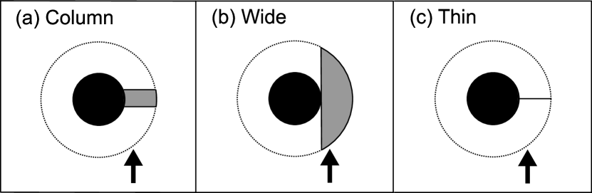
Figure 9: Possible geometries of the tongue. The arrows indicate the line of sight. Gray areas indicate the tongue and black areas indicate the cool core as seen perpendicular to our line of sight. (a) Column model. (b) Wide model. (c) Thin model.

The key uncertainty in the deprojection is the extent of the tongue along the line of sight. In Figure 9, we present three simple models of this extent. Firstly, we assumed that the extent of the tongue along the line of sight was the same as its transverse width (Fig. 9a); we refer to this as the “Column” model. Secondly, the line-of-sight depth of the tongue might be comparable to its radial extent from the cluster center, which would correspond to a cap-like structure seen end-on. As a specific model of this, we assumed that the tongue filled a $\pm 30^{\circ}$ sector centered on the tongue on the plane of the sky (Fig. 9b). We will refer to this as the “Wide” model for the tongue. Finally, the tongue might be very narrow along the line of sight (Fig. 9c, the “Thin” model). Based on the arguments about the origin of the tongue in Fujita et al. (2002), the Column model seems the more likely geometry. The results of the spectral fits for these models are shown in Table 1. In each case, $T_{1}$ and $Z_{1}$ are the temperature and abundance in the tongue, respectively. The values with subscript 2 refer to the ambient gas near the tongue.

As a more general means to determine the spectrum of the tongue without making any detailed models for its geometry, we assume that the projected emission from the tongue consists of projected emission from larger radii ($r>49\arcsec$) determined directly from spectra at larger radii, and a mixture of tongue and ambient emission from radii of $24\arcsec<r<49\arcsec$. Rather than specify anything about the ambient emission in this region, we simply fit the spectrum of tongue and ambient emission at these radii with a two-temperature model. The results for this less restrictive “2T” model are shown at the end of Table 1.

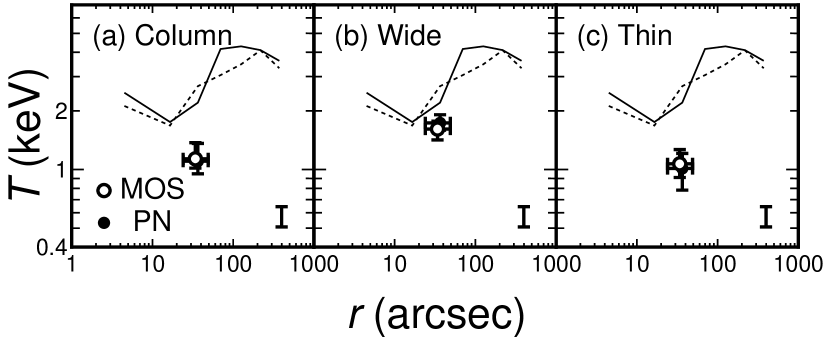
Figure 10: The same as Figure 5 but for the deprojection analysis. (a) Column model. (b) Wide model. (c) Thin model. The typical errors for the lines are shown by the bars at the lower right corners.

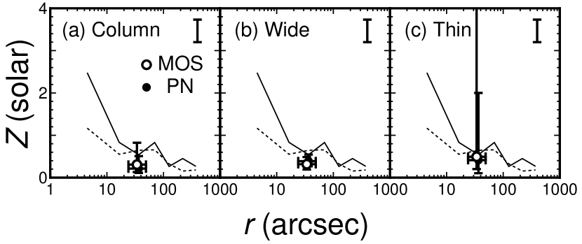
Figure 11: The same as Figure 10 but for metal abundance. The typical errors for the lines are shown by the bars at the upper right corners.

In all of the models, the temperature of the tongue is smaller than that of the surrounding regions (Fig. 10), which is the same result as that found with Chandra (Fujita et al., 2002). The most likely Column model, the Thin model, and the most general 2T model all are consistent with the temperature of the tongue region being $\sim$1.1 keV, while the ambient cluster gas at the same radius has a temperature of about 2.5 keV. The general consistency of the Column, Thin, and 2T temperatures suggests that the tongue actually is narrower along the line of sight than its radius out from the center of the cluster. Although the values for the abundance in the tongue ($\sim$0.4 solar) are generally smaller than those for the surrounding ICM ($\sim 0.6Z_{\sun}$; Fig. 11), the uncertainties in the abundance are quite large, and the abundance in the tongue is generally consistent with the ambient abundance within the 90% confidence error bars. Thus, we have no evidence for any significant difference in the abundance of the tongue and the ambient gas.

3.4 Spectra for the Radio Relic

In order to investigate the physical conditions in the radio relic, we extracted the X-ray spectrum from the region shown in Figure 2. This is the same as the region ‘R’ in Figure 10 in Fujita et al. (2002) that overlaps the radio relic. Based on Figure 2, the X-ray spectrum appears to be somewhat harder within the parts of the radio relic which are to the east of the tongue. The primary purpose of the spectral analysis is to detect or constrain the contributions to the spectrum of a non-thermal inverse Compton or a very hot thermal component. Since the number of photons from the region is not large, we simultaneously fitted the three spectra obtained by the three detectors (MOS1, MOS2, and PN). First, we fitted the spectra with a single-temperature MEKAL model with a variable absorption (1T model in Table 2). Then, we added a power-law component, representing the inverse Compton emission, to the 1T model (1TPL model). In the 1TPL model, the metal abundance was fixed to the best-fit value in the 1T model because it could not be constrained. An alternative explanation for any hard X-ray emission in the radio relic region might be hot thermal gas filling the region. To study this, we also fit a two-temperature model with a variable absorption (2T model). We assume that the metal abundances of the two thermal components are the same.

The results are shown in Table 2. They are consistent with the Chandra results (Fujita et al., 2002), although the uncertainties are smaller here. The single-temperature model (1T) does not give a good fit. Both the 1TPL and 2T models give better fits to the spectrum. Their difference in the best-fit $\chi^{2}$ is small, and it is difficult to decide which provides the better fit. The $0.3$–$10$ keV flux of the power-law component is $2.4\times 10^{-13}<F_{\rm PL}<5.4\times 10^{-13}\>\rm ergs\;cm^{-2}\>s^{-1}$. This is consistent with the Chandra limit ($F_{\rm PL}<7.1\times 10^{-13}\>\rm ergs\;cm^{-2}\>s^{-1}$; Fujita et al., 2002), but is an even tighter constraint. Since the relic is near the tongue, the X-ray emission from the tongue may affect the spectrum of the relic region because of the PSF effect (§3.1). However, since the amount of leaked photons from the tongue is less than 20% and the photon energy is small because of the low temperature of the tongue, they do not affect the hot or nonthermal emission from the relic region. What is more serious is the contribution of the projected hot ICM from the outer parts of the cluster. Assuming that the cluster is spherically symmetric outside the tongue and the relic, we found the emission from the projected hot ICM cannot be ignored, compared with the hot or nonthermal emission from the relic region. Thus, we regard the upper value of the flux ($F_{\rm PL}<5.4\times 10^{-13}$ ergs cm^-2 s^-1) as a secure upper limit on the nonthermal emission from the radio relic.

3.5 X-ray Spectra of Possible Weak Shock Regions

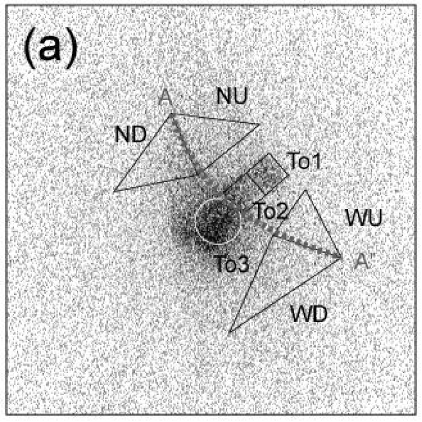
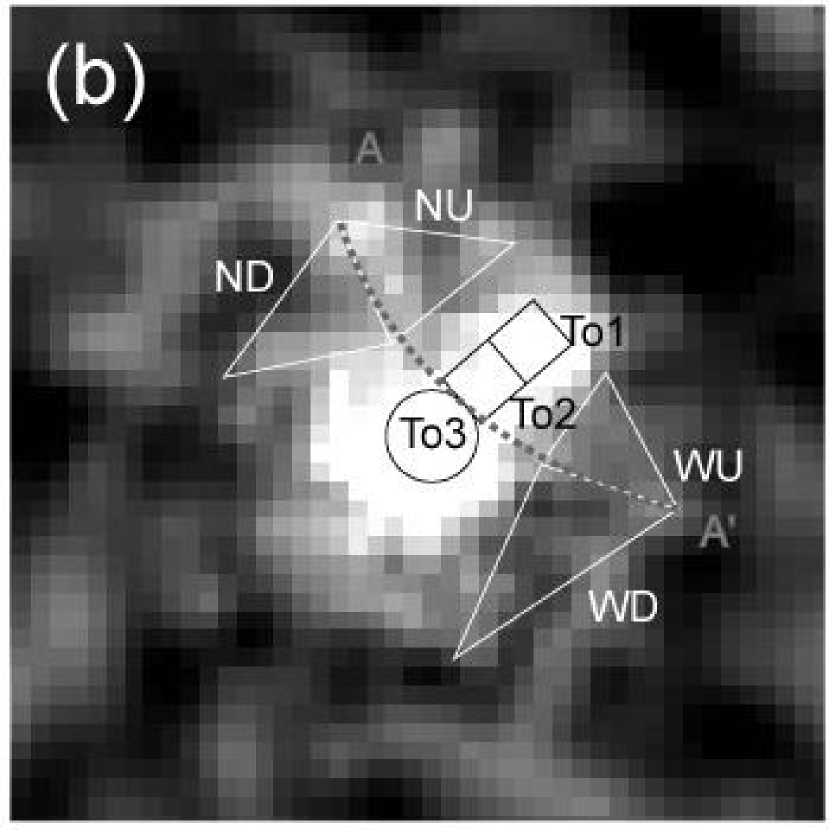
Figure 12: Regions for spectral analysis of the possible weak shock are overlaid on (a) a raw Chandra image and (b) the hardness ratio map (Fig. 2), where hard emission appears black. The image sizes are $3^{\prime}\times 3^{\prime}$. The curve AA^′ is a possible weak shock. The regions ND, NU, WD, WU are the north downstream, north upstream, west downstream and west upstream in the simple shock model presented. On the cluster core and tongue, To1 and To2 are upstream, while To3 is downstream.

The cool core of A133 has a bird-like structure, with “wings” extending toward north and west (Figs. 1b and 12a). The northwest edges of the wings form an arc (the curve AA^′). Based on the hardness ratio map (Fig. 12b), the temperatures in the wings may be somewhat higher than those of the neighboring faint regions (on the northwest side of the curve AA^′). Thus, the curve AA^′ may be a weak shock. Based on the hardness ratio map and the X-ray image, it appears that the shock is propagating from the southeast to the northwest. However, the increase in the hardness ratio around the curve AA^′ is fairly subtle. Moreover, if a spectrum consists of more than one temperature components, the relation between the hardness ratio and temperature is very complicated. Thus, in order to assess the existence of a possible temperature jump, we “measured” the temperatures by spectral fitting.

First, we investigated whether the shock is passing through the core and tongue. We chose three regions, To1, To2, and To3, shown in Figure 12. We fitted the spectra of each region obtained with MOS1, MOS2, and PN simultaneously because the photon counts from the regions are not large ($N\lesssim 1000$ for MOS1 and MOS2, and $\lesssim 3000$ for PN). We initially assumed one thermal component (MEKAL) with fixed Galactic absorption ($1.58\times 10^{20}\rm\>cm^{-2}$; Stark et al., 1992), and we refer to this model as ‘1T’.

The results of the fits are shown in Table 3. There are no significant differences in the temperatures between the expected upstream (To1 and To2) and downstream (To3) regions of the possible shock. However, the temperatures may be affected by projected hot ICM from the outer regions of the cluster. Thus, we added a hot thermal component representing the projected ICM to the 1T model. For this 2T_A model, we assume that the metal abundances of the two thermal components are the same because we cannot constrain the abundances without this assumption. We expect that the cooler component ($T_{1}$) represents the gas of the tongue. The temperature $T_{1}$ may rise by a factor of $1.5_{-0.3}^{+0.4}$ from region To2 to To3. In the 2T_B model, we forced the temperatures of the projected hotter component and the abundances to be the same for To1, To2, and To3. We assumed that the temperatures are 3.6 keV and the abundances are 0.7 $Z_{\sun}$, which are the averages of those for the 2T_A model. In this model, the error of the increase of the temperature $T_{1}$ from region To2 to To3 becomes smaller and the increase is a factor of $1.3_{-0.2}^{+0.0}$.

We also investigated the spectra of four wing regions, WU, WD, NU, and ND (west upstream, west downstream, etc.) shown in Figure 12. The curve AA’ corresponds to the small gap of the surface brightness seen on the Chandra image (Fig.1b). The four wing regions were chosen so that the temperature difference between the upstream and downstream regions was the largest by looking at the hardness ratio map (Fig. 12b). Moreover, we selected these regions because they are sufficiently far from the tongue that they are not affected by the tongue’s emission. Again, we fitted the spectra of each region obtained with MOS1, MOS2, and PN simultaneously. The results are presented in Table 4. For the single-temperature 1T model, there are no significant differences in the temperatures between the expected upstream (NU, WU) and downstream (ND, WD) regions of the possible shock. However, since the projection of the hot ICM in the outer region of the cluster may affect the results, we added another hot thermal component representing the projected ICM to the 1T models. Since the photon counts in these regions are particularly small, the temperature and metal abundance of the projected ICM were fixed at $T=4.0$ keV and $Z=0.6\>Z_{\sun}$, which are the average values of the ICM in the outer region of the cluster ($50\arcsec\lesssim r\lesssim 100\arcsec$; Figs. 3, 4, 7 and 8). Without fixing the projected component, we cannot constrain the cooler component. In order to reduce the number of free parameters further, we also fixed the abundance of the cooler component at $Z=0.6\>Z_{\sun}$. We fitted the spectra of the expected upstream (WU and NU) and downstream (WD and ND) regions with the two thermal components. The free parameters in this 2T model are the temperature and normalization of the cooler component and the normalization of the hotter component. However, while the temperature and normalization of the cooler component are independent in different regions, we adjusted the normalization of the hotter $4.0$ keV component in the downstream regions to that in the upstream regions in such a way that the normalization of the $4.0$ keV component in the WD (ND) region is assumed to be that in the WU (NU) region multiplied by the ratio of the area of WD to that of WU (the area of ND to that of NU). This means that the spectral contribution from the projected hotter component per unit area is the same for the WD (ND) and WU (NU) regions. The results are shown in Table 4. The spectra of the upstream and downstream regions are fitted simultaneously contrary to the 1T models. Therefore, for the 2T models, the degree of freedom and $\chi^{2}$ of the WD and WU (ND and NU) are the same and much larger than those for the 1T models (Table 4). For the cooler component in the west wing, the temperature rises from regions WU to WD by a factor of $2.3\pm 0.6$. For the north wing, we did not find evidence for a temperature change.

4 Discussion

4.1 Cold Front

The SE temperature jump found by us corresponds to the jump in surface brightness as seen in Chandra data (Fujita et al., 2002). Deprojection analysis showed that the density increases there by a factor of 1.3 from the outer to the inner region (Fig. 7 in Fujita et al., 2002). On the other hand, the temperature decreases by a factor of $1.4$ from the outer to the inner region. If we average the MOS and PN data about the temperature jump, the ratio of the pressures on the sides of the jump is $0.95\pm 0.11$, which is consistent with a continuous pressure across the jump. Thus, this jump may be classified as a “cold front”, and is similar to the one found in A1795 (Markevitch, Vikhlinin, & Mazzotta, 2001). From equation (2) in Vikhlinin et al. (2001), we found an upper limit of $U\leq 230\>\rm km\>s^{-1}$ for the relative velocity. In this estimation, we assumed the density and the temperature just inside the jump to be the same as those at the contact discontinuity. We estimated the gas pressure far upstream from the cold front by extrapolating the density and temperature inward from those determined at radii $r\sim 40-60^{\prime\prime}$ in the direction of the cold front.

4.2 Weak Shock

A detailed spectral analysis showed that the bird-like feature of the cool core seems to be a weak shock (§3.5). In fact, the direction of the bend of the curve AA^′ is consistent with this idea. When a shock passes the cool core from the southeast to the northwest, the velocity of the central part of the shock that passes through the cool core is smaller than the velocity of the part of the shock that passes around the core, because of the larger pressure and lower temperature of the core (See Fig. 11 in Churazov et al., 2003). It is this differential velocity that bends the shock.

In the core and tongue, the temperature rises from the region To2 to To3 by a factor of $1.3_{-0.2}^{+0.0}$ in the model 2$\rm T_{B}$ (Table 3). The Mach number of the shock is $1.3_{-0.2}^{+0.0}$ as derived from the Rankine-Hugoniot relation:

$$\frac{T_{d}}{T_{u}}=\frac{[2\gamma M_{u}^{2}-(\gamma-1)][(\gamma-1)M_{u}^{2}+2]}{(\gamma+1)^{2}M_{u}^{2}}\>,$$ (1)

where $T_{u}$ is the upstream temperature, $T_{d}$ is the downstream temperature, $\gamma(=5/3)$ is the adiabatic index, and $M_{u}$ is the upstream Mach number. Thus, the shock is marginally detected. On the other hand, the temperature ratio at the western shock is $2.3\pm 0.6$ (Table 4), and the Mach number of the shock is $1.6$–$2.6$ from the Rankine-Hugoniot relation. However, the evidence of the western shock is based on keeping the temperatures of the projected hot component fixed. There is no such evidence when all temperatures are left unrestricted. (§3.5).

The shape of the shock front shows that the shock is not directly related to the central AGN of the cluster (Fig. 1b). Thus, it may be different from the weak shocks found in the core of the Perseus cluster (Fabian et al., 2003). It is more possible that the shock originated outside the core region and propagated into the core. If so, this is the first time that a sign of this kind of shock is found in a cluster core. The shock might have formed in a former cluster merger. Alternatively, it might have formed through steepening of the fronts of sound waves with large amplitudes produced by ICM motion in the cluster. This is because the sound speed of the compressed gas is higher than that in the rarefied part, so the waves will steepen over a few wavelengths (e.g. Fig. 55.1 in Mihalas & Mihalas, 1984). Recently, Fujita, Suzuki, & Wada (2004) showed analytically and numerically that sound waves formed outside a cluster core steepen and become weak shocks in the core. These shocks heat the cool core and increase the cooling time of the gas in the core, which may solve the cooling flow problem. Some of the complicated X-ray structures in the core found in the Chandra observations (Fig. 1b) may be produced by the passage of this shock (Fujita, Matsumoto, & Wada, 2004). We note that the regions around the curve AA^′ we took for the spectral analysis are fairly large. Therefore, the temperature jump we found may not be as sharp as expected for a shock. In this case, the gradient of the temperature and surface brightness could be explained by a sound wave. Since the amplitude represented by the temperature gradient is relatively large, the wave would become a weak shock as it propagates only a few wavelengths (Mihalas & Mihalas, 1984).

4.3 The Origin of the X-ray Tongue

Fujita et al. (2002) discussed several models for the origin of the tongue: (1) a cooling wake; (2) a cluster merger; (3) Kelvin-Helmholtz (KH) instabilities; or (4) a buoyant radio bubble. In the cooling-wake scenario the tongue is the gas cooling from the hot ICM, attracted into a wake along the path of the moving cD galaxy (David et al., 1994; Fabian et al., 2001). The cluster-merger scenario predicts that the tongue is formed through convection induced by a cluster merger (Ricker & Sarazin, 2001). In the KH-instability scenario, the cool core is moving relative to the surrounding hot ICM. As a result, KH instabilities develop around the core and produce the tongue. In the buoyant bubble scenario, the radio relic is an old radio lobe, which is moving outward in the cluster gravitational potential. This buoyant radio bubble lifts up cooler gas from the cluster center (e.g. Churazov et al., 2001; Quilis et al., 2001; Brüggen & Kaiser, 2001). In the following, we compare each of these scenarios using our combined XMM-Newton and Chandra data.

4.3.1 A Cooling Wake

Fujita et al. (2002) concluded that the cooling-wake scenario is not favored by the steep temperature gradient on both sides of the tongue; the temperature should be continuous if the cold gas of the tongue is a result of the cooling flow from the surrounding ICM. The XMM-Newton results are consistent with this, albeit with poorer spatial resolution. However, the XMM-Newton observations, with their information on the metal abundance, may provide another clue. If the metal abundance around the tongue were also discontinuous, it would strengthen the previous conclusion and make the cooling wake model even more unlikely. Table 1 and Figure 11 show that, although the best-fit abundance in the tongue is generally somewhat lower than that in the ambient gas, the two are consistent within the uncertainties. Thus, based only on the metal abundance, we cannot reject the cooling-wake scenario.

4.3.2 Cluster Merger

Fujita et al. (2002) also concluded that the cluster merger scenario is not suitable to explain the origin of the tongue since no clear evidence of a shock was seen, neither in the image, nor in the X-ray hardness map, nor in the Chandra spectra. However, by comparing the XMM-Newton and Chandra observations, we have found a possible weak shock in the cool core (§3.5). Moreover, if the ratio of the masses of the merging clusters is large (minor merger), we may not necessarily expect to find clear structures, such as a strong shock, associated with the merger. Gómez et al. (2002) performed numerical simulations of the head-on merger of a cooling flow cluster with an infalling subcluster of galaxies. They adopted relatively high mass ratios of 16:1 and 4:1. Since they included the effect of gas cooling, the central density of the cluster is high. Because of this, in some cases the gas of the subcluster cannot penetrate the cooling core of the larger cluster, while the dark matter can. As a result, the cool core of the cluster is not destroyed by the merger. Well after the merger ($\gtrsim 1$ Gyr), the cluster becomes spherical (Gómez et al., 2002). However, the oscillation of the ICM may elongate the core and produce a tongue-like structure (Fig. 6 in Gómez et al., 2002). Moreover, the sloshing of the ICM around the core could produce the temperature jump at the southeast edge of the core, and a temperature jump of this type may exist without a pressure discontinuity (Markevitch et al., 2001; Churazov et al., 2003). Thus, if the mass ratio of the merging clusters is large, a cluster merger remains a candidate for the origin of the tongue and the temperature jump.

4.3.3 Kelvin-Helmholtz Instability

The KH instability scenario seemed plausible in Fujita et al. (2002). However, these authors could not estimate the velocity of the cool core from Chandra data, and thus they assumed it was sufficient to produce the instability. In § 4.1 of the present paper, we derived an upper limit on the velocity of the cool core based on the XMM-Newton data. The minimum velocity for the development of KH instabilities is,

$$U_{\rm KH}\equiv\sqrt{\frac{k_{B}T_{\rm in}}{\pi\mu m_{H}}\frac{D^{2}-1}{D}}=230\rm\>km\>s^{-1}\,,$$ (2)

where $k_{B}$ is the Boltzmann constant, $T_{\rm in}$ is the temperature on the side of the temperature jump which is closer to the cluster center, $m_{H}$ is the mass of the hydrogen atom, and $D\;(\geq 1)$ is the density contrast at the edge of the cool core (Fujita et al., 2002). On the other hand, we found the velocity of the cool core is $U<230\rm\>km\>s^{-1}$ (§4.1), which is smaller than $U_{\rm KH}$. This means that KH instabilities are unlikely to develop around the cool core.

4.3.4 Buoyant Radio Bubble

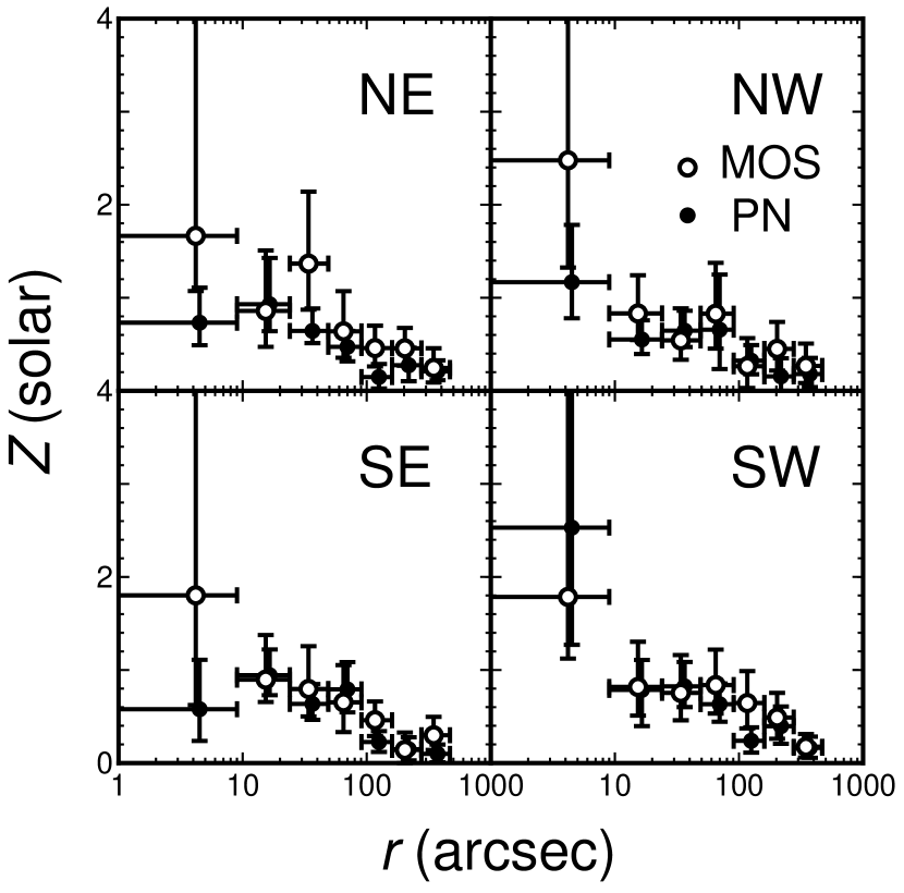
Figure 8: The same as Figure 4 but for the deprojection analysis.

Chandra data had shown that there is an X-ray deficit in the region around the radio relic northwest of the cluster center (Fujita et al., 2002). Thus, there seems to be a bubble in the ICM. If the tongue is the gas uplifted by the buoyant bubble, the properties of its gas should be the same as those at the cluster center. The metal abundance at the cluster center is $Z\gtrsim 1.0\>Z_{\sun}$ (Fig. 8). As discussed in §4.3.1, although the best-fit abundance in the tongue is lower, the uncertainties are large enough to be consistent with those at the cluster center, at least if the volume of the tongue is small (Fig.  11c). Thus, this scenario is still plausible.

Slee et al. (2001) estimated that the age of the relic is $t_{\rm radio}=4.9\times 10^{7}$ yr. If the cD galaxy were located at the position of the relic when the relic was formed, the velocity of the galaxy must be $U\gtrsim 700\>\rm km\>s^{-1}$ (Fujita et al., 2002). This is inconsistent with the velocity of $U<230\rm\>km\>s^{-1}$ inferred from the present observations. However, buoyancy provides a viable transport mechanism for the relic, since the required velocity of the bubble is consistent with the results of numerical simulations (e.g., Churazov et al., 2001).

4.4 The Radio Relic

We found an upper limit on the nonthermal X-ray emission from the radio relic of $F_{\rm PL}<5.4\times 10^{-13}$ ergs cm^-2 s^-1. From this limit, we can derive a lower limit on the magnetic field in the relic by comparing this limit to the inverse Compton emission expected from the radio-emitting electrons. We adopt an X-ray photon index of 1.8 and a radio flux density of $35.5\pm 4.3$ Jy at 80 MHz (Slee et al., 2001). Using the standard expressions for the inverse Compton and synchrotron emission assuming a power-law electron energy distribution (e.g., Sarazin, 1986), we can constrain the required magnetic field in the relic as $B\geq 1.5$ $\mu$G, which is consistent with the Chandra result ($B\geq 1.2$ $\mu$G; Fujita et al., 2002). This value is at least consistent with the magnetic field of $14.4\>\mu$G derived from minimum-energy arguments (Slee et al., 2001).

5 Conclusions

We have presented the results of an XMM-Newton observation of the cluster of galaxies A133. We found a probable cold front to the southeast of the cool core. The pressure around the front shows that the relative velocity of the core with respect to the rest of the cluster is very small ($U<230\rm\>km\>s^{-1}$). This cold front was first identified as a surface brightness discontinuity with Chandra, but only with XMM-Newton spectra were we able to determine the nature of this feature.

The Chandra image of A133 showed a complex, bird-like morphology in the cluster core. Based on the XMM-Newton spectra and hardness ratio maps, we argue that the wings of this structure are a weak shock front. However, this evidence is marginal as it is based keeping the temperatures of the projected hot component fixed, and the evidence disappears when all temperatures are left free. The shock appears to be propagating from the southeast to the northwest. Its curved shape suggests that it has already passed through the cluster core, and that the central portion of the shock was retarded by the higher density at the cluster center. This morphology is not consistent with the shock arising from the active nucleus of the cluster’s central cD galaxy, unlike the weak shocks which have been seen in the Chandra image of the Perseus cluster (Fabian et al., 2003). To our knowledge, the morphology and origin of this shock are new features which have not been observed in other clusters so far. This shock may be heating the cluster core.

Our previous Chandra observations showed a “tongue” of relatively cool gas extending from the center of the cD to the center of the radio relic. We have used XMM-Newton spectra to test various models for the origin of this tongue. Both the Chandra and XMM-Newton observations indicate that the temperature in the tongue drops discontinuously at its sides, which is inconsistent with it being a cooling wake. A discontinuity of the metal abundance would be a further argument against this origin, but the XMM-Newton spectra do not allow any firm conclusion about such a discontinuity. The small velocity of the core, as determined from the pressure profile near the cold front, is inconsistent with the possibility that the tongue is formed through Kelvin-Helmholtz instabilities around the core. The tongue may well be gas which has been uplifted by a buoyant radio bubble including the radio relic in the northwest of the core. This model predicts that the metal abundances in the tongue be high and comparable to those at the very center of the cluster, where the gas would have originated. Despite the fact that the best-fit abundances in the tongue derived from XMM-Newton spectra are lower than predicted, the uncertainties do allow for high abundances as well. Thus, a buoyant bubble is still a promising candidate for the origin of the tongue. Our XMM-Newton observation has revived interest in the possibility that the tongue results from a cluster merger. Previously, the main argument against this model was the lack of evidence for any merger-related shocks. Our discovery of a likely weak merger shock supports this model, which probably requires a very unequal merger with a large mass ratio between the main cluster and the merging subcluster.

There is no clear evidence of nonthermal inverse Compton emission from the radio relic in the X-ray band. The upper limit on the inverse Compton contribution based on our XMM-Newton spectra implies a lower limit on the magnetic field in the radio relic of $B\geq 1.5$ $\mu$G.

Table 1: Deprojected Spectra of the Tongue

	$T_{1}$	$T_{2}$	$Z_{1}$	$Z_{2}$	$\chi^{2}$/dof
Model	(keV)	(keV)	($Z_{\sun}$)	($Z_{\sun}$)
Column (MOS)	$1.1^{+0.3}_{-0.1}$	2.2	$0.31^{+0.18}_{-0.51}$	0.54	0.886 (22.2/25)
Column (PN)	$1.1^{+0.3}_{-0.1}$	2.6	$0.21^{+0.30}_{-0.10}$	0.65	0.950 (32.3/34)
Wide (MOS)	$1.6^{+0.2}_{-0.2}$	$\cdots$	$0.32^{+0.17}_{-0.13}$	$\cdots$	1.11 (27.6/25)
Wide (PN)	$1.7^{+0.2}_{-0.1}$	$\cdots$	$0.39^{+0.15}_{-0.12}$	$\cdots$	0.950 (32.3/34)
Thin (MOS)	$1.1^{+0.2}_{-0.2}$	2.2	$0.49^{+\infty}_{-0.29}$	0.54	0.820 (20.5/25)
Thin (PN)	$1.0^{+0.2}_{-0.2}$	2.6	$0.41^{+1.59}_{-0.31}$	0.65	1.10 (37.5/34)
2T (MOS)	$1.1^{+0.3}_{-0.3}$	$2.6^{+1.9}_{-0.6}$	$0.51^{+\infty}_{-0.32}$	0.54	0.865 (29.9/23)
2T (PN)	$0.8^{+0.6}_{-0.3}$	$2.0^{+0.8}_{-0.2}$	$0.15^{+0.60}_{-0.12}$	0.65	0.859 (27.5/32)

Note. — The cooler component ($T_{1}$, $Z_{1}$) represents the gas of the tongue, and the hotter component ($T_{2}$, $Z_{2}$) represents the surrounding gas.

Table 2: Spectra for the Radio Relic Region

	$T_{1}$	$T_{2}$	$Z$	$\Gamma$	$N_{\rm H}$	$\chi^{2}$/dof
Model	(keV)	(keV)	($Z_{\sun}$)		($\times 10^{20}\rm\;cm^{-2}$)
1T	$2.8_{-0.1}^{+0.1}$	$\cdots$	$0.72_{-0.12}^{+0.15}$	$\cdots$	$0.93_{-0.64}^{+0.67}$	1.18 (189.6/160)
1TPL	$2.1_{-0.2}^{+0.1}$	$\cdots$	0.72	$1.8_{-0.2}^{+0.1}$	$2.51_{-1.15}^{+1.38}$	1.05 (167.0/159)
2T	$1.6_{-0.5}^{+0.6}$	$3.6_{-0.6}^{+\infty}$	$0.65_{-0.27}^{+0.23}$	$\cdots$	$0.74_{-0.8}^{+0.6}$	1.06 (167.7/158)

Table 3: Spectra of the Core and Tongue

		$T_{1}$	$T_{2}$	$Z$	$\chi^{2}$/dof
Region	Model	(keV)	(keV)	($Z_{\sun}$)
To1	1T	$1.6^{+0.1}_{-0.1}$	$\cdots$	$0.38^{+0.12}_{-0.09}$	1.89 (68.1/36)
To1	2TA	$1.1^{+0.3}_{-0.2}$	$2.4^{+\infty}_{-0.4}$	$0.57^{+0.40}_{-0.33}$	1.38 (46.8/34)
To1	2TB	$1.3^{+0.1}_{-0.1}$	3.6	0.7	1.54 (55.3/36)
To2	1T	$2.0^{+0.1}_{-0.2}$	$\cdots$	$0.64^{+0.17}_{-0.14}$	1.51 (80.0/53)
To2	2TA	$1.1^{+0.3}_{-0.1}$	$2.8^{+0.8}_{-0.4}$	$0.81^{+0.31}_{-0.18}$	1.00 (51.2/51)
To2	2TB	$1.3^{+0.1}_{-0.1}$	3.6	0.7	1.00 (53.0/53)
To3	1T	$2.0^{+0.1}_{-0.1}$	$\cdots$	$0.75^{+0.12}_{-0.08}$	1.41 (205.9/146)
To3	2TA	$1.7^{+0.1}_{-0.3}$	$5.6^{+\infty}_{-2.4}$	$0.71^{+0.16}_{-0.11}$	1.30 (187.0/144)
To3	2TB	$1.7^{+0.1}_{-0.1}$	3.6	0.7	1.29 (187.6/146)

Table 4: Spectra around the Weak Shock

		$T$	$Z$	$\chi^{2}$/dof
Region	Model	(keV)	($Z_{\sun}$)
WU	1T	$3.2_{-0.4}^{+0.4}$	$0.35_{-0.19}^{+0.31}$	0.955 (33.4/35)
	2T	$0.9_{-0.2}^{+0.2}$	0.6	0.990 (122.7/124)
WD	1T	$3.2_{-0.2}^{+0.2}$	$0.61_{-0.15}^{+0.17}$	1.08 (95.8/88)
	2T	$2.0_{-0.2}^{+0.4}$	0.6	0.990 (122.7/124)
NU	1T	$2.7_{-0.2}^{+0.2}$	$0.50_{-0.14}^{+0.17}$	1.50 (102.0/68)
	2T	$2.2_{-0.5}^{+0.2}$	0.6	1.12 (157.0/140)
ND	1T	$2.7_{-0.2}^{+0.2}$	$0.62_{-0.15}^{+0.19}$	1.06 (75.1/71)
	2T	$2.1_{-0.4}^{+0.5}$	0.6	1.12 (157.0/140)

Note. — The shock region temperatures and abundances in the 2T model are those of the cooler component. The 2T fits have much more degrees freedom than the 1T fits because the 2T fits are simultaneous fits of the upstream and downstream regions whereas 1T fits are individual fits (see text).

Figure 1: (a) Adaptively smoothed, combined MOS1-MOS2-PN image of A133 in the energy range of $0.3-2$ keV, corrected for background, exposure, and vignetting. North is up and east is left. The linear artifacts are due to an imperfect exposure correction near the chip boundaries. (b) Adaptively smoothed Chandra image of the central $2^{\prime}\times 2^{\prime}$ region of A133, corrected for background, exposure, and vignetting. The region shown in Figure 1b is indicated as a solid-line square in Figure 1a. The curve AA^′ is a possible weak shock (see §3.5). The tongue and AGN are indicated by arrows.

Figure 2: Color map of hardness ratio of the central $3^{\prime}\times 3^{\prime}$ region of A133, based on the ratio of the combined MOS1-MOS2-PN count rates in the energy bands $0.3$–$2.0$ keV and $2.0$–$10$ keV. The map has been corrected for background, exposure, and vignetting, and is adaptively smoothed. Soft emission appears yellow and hard emission black. Also shown are surface brightness contours from Chandra (see Fig. 1b). The thin white dotted lines show the 4 quadrants used for the analysis of the profiles of temperature and abundance (§3.1 & 3.2). The dashed line shows the radio relic region (see §3.4). The thick white solid line in the SE sector is a cold front (see §4.1).

Figure 3: Projected temperature as a function of radius from the XMM-Newton observation. Temperatures obtained from the two MOS detectors are shown as open circles, while temperatures obtained from the PN are shown as solid circles. A temperature jump corresponding to a cold front is shown by an arrow in the SE panel.

Figure 4: Projected metal abundance as a function of radius in the XMM-Newton observation. Abundances obtained from MOS are shown as open circles, and abundances obtained from PN are shown as solid circles.

Figure 5: (a) Projected temperature of the tongue. A temperature obtained from MOS is shown as an open circle; the temperature from PN is almost exactly the same, and this point lies beneath the MOS point. The solid line shows the best fit temperatures obtained from MOS in the NW sector shown in Figure 3, excluding the emission from the tongue. The dotted line is that obtained from PN. The typical error for the lines are shown by the bar at the lower right corner. (b) The same as Figure (a) but for metal abundance.

Figure 6: Projected temperature as a function of radius for the SE sector for MOS. Open circles are the same as those in Figure 3. Open triangles are the temperature profile corrected for the PSF.

Figure 7: The same as Figure 3 but for the deprojection analysis.

References

- Blanton et al. (2003) Blanton, E. L., Sarazin, C. L., & McNamara, B. R. 2003, ApJ, 585, 227
- Brüggen & Kaiser (2001) Brüggen, M. & Kaiser, C. R. 2001, MNRAS, 325, 676
- Buote (2000) Buote, D. A. 2000, MNRAS, 311, 176
- Churazov et al. (2001) Churazov, E., Brüggen, M., Kaiser, C. R., Böhringer, H., & Forman, W. 2001, ApJ, 554, 261
- Churazov et al. (2003) Churazov, E., Forman, W., Jones, C.,& Böhringer, H. 2003, ApJ, 590, 225
- David et al. (1994) David, L. P., Jones, C., Forman, W., & Daines, S. 1994, ApJ, 428, 544
- Fabian et al. (2003) Fabian, A. C., Sanders, J. S., Allen, S. W., Crawford, C. S., Iwasawa, K., Johnstone, R. M., Schmidt, R. W., & Taylor, G. B. 2003, MNRAS, 344, L43
- Fabian et al. (2001) Fabian, A. C., Sanders, J. S., Ettori, S., Taylor, G. B., Allen, S. W., Crawford, C. S., Iwasawa, K., & Johnstone, R. M. 2001, MNRAS, 321, L33
- Fujita et al. (2002) Fujita, Y., Sarazin, C. L., Kempner, J. C., Rudnick, L., Slee, O. B., Roy, A. L., Andernach, H., & Ehle, M. 2002, ApJ, 575, 764
- Fujita et al. (2004) Fujita, Y., Matsumoto, T., & Wada, K. 2004, ApJ Letters, in press (astro-ph/0407368)
- Fujita et al. (2004) Fujita, Y., Suzuki, T. K., & Wada, K. 2004, ApJ, 600, 650
- Ghizzardi (2001) Ghizzardi, S. 2001, http://xmm.vilspa.esa.es/docs/documents/CAL-TN-0022-1-0.ps.gz
- Gómez et al. (2002) Gómez, P. L., Loken, C., Roettiger, K., & Burns, J. O. 2002, ApJ, 569, 122
- Jansen et al. (2001) Jansen, F. et al. 2001, A&A, 365, L1
- Krywult et al. (1999) Krywult, J., MacGillivray, H. T., & Flin, P. 1999, A&A, 351, 883
- Majerowicz et al. (2002) Majerowicz, S., Neumann, D. M., & Reiprich, T. H. 2002, A&A, 394, 77
- Markevitch et al. (2001) Markevitch, M., Vikhlinin, A., & Mazzotta, P. 2001, ApJ, 562, L153
- Mihalas & Mihalas (1984) Mihalas, D., & Mihalas, W. B. 1984, Foundations of Radiation Hydrodynamics (New York: Oxford Univ. Press)
- Quilis et al. (2001) Quilis, V., Bower, R. G., & Balogh, M. L. 2001, MNRAS, 328, 1091
- Reiprich et al. (2004) Reiprich, T. H., Sarazin, C. L., Kempner, J. C., & Tittley, E. 2004, ApJ, 608, 179
- Ricker & Sarazin (2001) Ricker, P. M. & Sarazin, C. L. 2001, ApJ, 561, 621
- Rizza et al. (2000) Rizza, E., Loken, C., Bliton, M., Roettiger, K., Burns, J. O., & Owen, F. N. 2000, AJ, 119, 21
- Sarazin (1986) Sarazin, C. L. 1986, Rev. Mod. Phys., 58, 1
- Slee et al. (2001) Slee, O. B., Roy, A. L., Murgia, M., Andernach, H., & Ehle, M. 2001, AJ, 122, 1172
- Stark et al. (1992) Stark, A. A., Gammie, C. F., Wilson, R. W., Bally, J., Linke, R. A., Heiles, C., & Hurwitz, M. 1992, ApJS, 79, 77
- Strüder et al. (2001) Strüder, L. et al. 2001, A&A, 365, L18
- Turner et al. (2001) Turner, M. J. L. et al. 2001, A&A, 365, L27
- Vikhlinin et al. (2001) Vikhlinin, A., Markevitch, M., & Murray, S. S. 2001, ApJ, 551, 160
- Way et al. (1997) Way, M. J., Quintana, H., & Infante, L. 1997, AJ, submitted (astro-ph/9709036)
- White et al. (1997) White, D. A., Jones, C., & Forman, W. 1997, MNRAS, 292, 419