Effects of Destriping Errors on Estimates of the CMB Power Spectrum

Abstract

Destriping methods for constructing maps of the Cosmic Microwave Background (CMB) anisotropies have been investigated extensively in the literature. However, their error properties have been studied in less detail. Here we present an analysis of the effects of destriping errors on CMB power spectrum estimates for Planck-like scanning strategies. Analytic formulae are derived for certain simple scanning geometries that can be rescaled to account for different detector noise. Assuming Planck-like low-frequency noise, the noise power spectrum is accurately white at high multipoles ($\ell\lower 2.15277pt\hbox{$\;\buildrel>\over{\sim}\;$}50$). Destriping errors, though dominant at lower multipoles, are small in comparison to the cosmic variance. These results show that simple destriping map-making methods should be perfectly adequate for the analysis of Planck data and support the arguments given in an earlier paper in favour of applying a fast hybrid power spectrum estimator to CMB data with realistic ‘$1/f$’ noise.

Key words: Methods: data analysis, statistical; Cosmology: cosmic microwave background, large-scale structure of Universe

1 Introduction

The problem of constructing a map of the CMB anisotropies from a set of time-ordered data (TOD) has been studied by many authors. The methods can be broadly divided into two classes: ‘optimal’ methods that provide a least squares map making solution (e.g. Wright 1996; Wright et al. 1996; Tegmark 1997a,b; Borrill et al. 2001; Natoli et al. 2001; Doré et al. 2001) and approximate ‘destriping’ methods (e.g. Burigana et al. 1997; Delabrouille 1998; Maino et al. 1999; Revenu et al. 2000; Keihänen et al. 2003). A brute force application of ‘optimal’ methods requires the inversion of large matrices and is computationally impractical for large TODs such as those expected from WMAP and Planck. As a result, iterative algorithms have been developed (e.g. Wright et al. 1996; Natoli et al. 2001; Doré et al. 2001) which do not require matrix inversions. Nevertheless, for Planck-sized datasets, these iterative algorithms are computationally expensive and require the use of supercomputers.

Destriping algorithms are well suited to a Planck-type scanning strategy in which the sky is scanned many times on rings. The TOD can then be averaged on rings and the effects of low frequency noise noise approximated by a constant offset for each ring. The offsets can be determined from the ring overlaps. Destriping algorithms are conceptually simple and computationally fast. Even for Planck-sized TODs it is practical to apply destriping map making methods on many thousands of simulations to test the effects of various systematic errors (see e.g. Poutanen et al. 2004).

The motivation for this paper is twofold. Firstly, although a number of authors have investigated destriping algorithms, almost all of this work has been numerical. A notable exception is the paper by Stompor and White (2004) who present an analysis of destriping errors for some simple scanning strategies. One of the aims of this paper is to develop on the work of Stompor and White and to derive an analytic model of the effects of destriping errors on the CMB power spectrum for Planck-like scanning strategies. This is useful because it helps in developing an understanding of the map-making process and how the errors depend on the parameters of the experiment. This analysis also sheds light on the differences between destriping and ‘optimal’ map-making methods. In particular, whether the extra computational cost and complexity of an optimal method actually produces any significant improvement on simple destriping.

The second motivation for this paper follows from the need to compute estimates of the CMB power spectrum, $C_{\ell}$, rapidly and acurately. In an earlier paper (Efstathiou 2004, hereafter E04) a fast hybrid estimator was developed that combines a quadratic maximum likelihood estimator at low multipoles with a set of ‘pseudo-$C_{\ell}$’ estimates at high multipoles with different pixel weightings. In E04 this method was tested against numerical simulations that used a realistic scanning strategy for Planck, but assumed uncorrelated white noise. In this approximation, the hybrid estimator was shown to be very close to optimal and, importantly, can provide an accurate estimate of the covariance matrix $\langle\Delta C_{\ell}\Delta C_{\ell^{\prime}}\rangle$. However, in a realistic experiment, striping errors will introduce correlations in the noise. The question then arises as to whether the hybrid estimator is applicable, for example, is there a natural angular scale below which the noise can be assumed white, and if so, what fixes this scale?

Our goal, therefore, is to investigate the effects of destriping errors on the CMB power spectrum for realistic scanning strategies and noise models. It should be emphasised that we do not attempt to develop a new map making technique, nor to investigate ‘real world’ complexities such as asymmetric beams, positional errors or non-stationary noise, though we will comment on how some of these aspects may effect our results.

2 Overview of Map Making with Destriping

We denote the noise contribution to the TOD by $n(t)$, which is considered to be a vector specified at integer values of the sampling frequency $t_{\rm samp}$, i.e. $n_{i}=n(it_{\rm samp})$, $i=1,\dots N$. The discrete Fourier transform of the noise TOD is denoted $\hat{n}(\nu)$ and the power spectrum $\langle|\hat{n}(\nu)|^{2}\rangle$ is assumed to be of the form

$$P_{n}(\nu)={\sigma^{2}_{n}\over T\nu_{\rm max}}\left(1+{\nu_{\rm knee}\over\nu}\right),\qquad{1\over T}\leq\nu\leq{1\over 2t_{\rm samp}},$$ (1)

where $\nu_{\rm knee}$ is the ‘knee frequency’and $T$ is the total length of the time-stream. The variance of the noise contribution given the power spectrum (1) is

$$\langle|n(t)|^{2}\rangle=\sigma^{2}_{n}\left(1+\nu_{\rm knee}{\rm\ln}(0.5T/t_{\rm samp})\right),$$ (2)

and thus $\sigma^{2}_{n}$ fixes the overall amplitude of the noise and is equal to the variance of white noise in the limit $\nu_{\rm knee}\rightarrow 0$.

The actual TOD is the sum of the true sky signal $s_{p}$ and the noise TOD

$$x_{i}=P_{ip}s_{p}+n_{i},$$ (3)

where $P_{ip}$ is a pointing matrix mapping a pixel $p$ on the sky to the pixel $i$ in the TOD. For a Planck-type scanning strategy, the same circle on the sky is mapped $N_{\rm repoint}=60$ times before the satellite is repointed. We will denote the spin period by $t_{\rm spin}$ and the repointing time interval by $t_{\rm repoint}$ ($\equiv N_{repoint}t_{\rm spin}$). As explained in the introduction, the main aim of this paper is not to develop an ‘optimal’ map-making technique, but rather to gain an intuitive understanding of the error properties of simple destriping map making methods. We therefore assume perfect pointing and simply average the TOD on each scanning ring:

$$\bar{x}_{i}^{k}=\sum_{j=0}^{N_{\rm repoint}-1}x_{i+jN_{\rm ringpix}+(k-1)N_{\rm repoint}N_{\rm ringpix}},\qquad N_{\rm ringpix}\equiv t_{\rm spin}/t_{\rm samp}.$$ (4)

where $N_{\rm ringpix}$ is the number of pixels withing a single ring pixel and $\bar{x}_{i}^{k}$ is the mean vaue of the TOD in ring pixel $i$ of ring $k$. This simple averaging is the maximum likelihood solution for map making on a ring if the pointing is assumed to be perfect. It is possible to improve on (4) to account for imperfect pointing by solving the maximum likelihood equations to reconstruct a map from all scanning rings within a single pointing period (see, for example, van Leeuwen et al. 2002).

    Table 1: Notation and parameters

symbol	description	value
$N_{\rm ring}$	number of  rings	$2160$
$N_{\rm ringpix}$	number of  pixels  per  ring	$2160$
$N_{\rm repoint}$	number of  rings  per  repointing	$60$
$T$	length  of  TOD	$7.78\;{\rm Ms}$
$t_{\rm repoint}$	pointing  period	$3600\;{\rm s}$
$t_{\rm spin}$	spin  period	$60\;{\rm s}$
$t_{\rm samp}$	sampling period	$27.78\;{\rm ms}$
$\nu_{\rm spin}$	spin  frequency	$16.67\;{\rm mHz}$
$\nu_{\rm knee}$	knee  frequency	$30.00\;{\rm mHz}$
$\nu_{\rm max}$	maximum  frequency	$18.00\;{\rm Hz}$
$\sigma_{N}$	noise amplitude	$1.36\;{\rm mK}$
$\Delta\theta_{\rm ring}$	ring  width	$10\;{\rm arcmin}$
$\Delta\theta_{\rm ringpix}$	size  of ring  pixel	$10\;{\rm arcmin}$
$\Delta\theta_{\rm map}$	size  of map  pixel	$15\;{\rm arcmin}$
$\theta_{\rm beam}$	beam  width FWHM	$30\;{\rm arcmin}$
$N_{\rm map}$	number  of  map  pixels	$659676$
$x_{i}$	signal+noise  in  TOD  pixel $i$
$\bar{x}_{i}^{k}$	mean  signal+noise  in  pixel $i$ of  ring $k$
$\epsilon_{k}$	offset  of  ring $k$
$m_{p}$	map  pixel $p$

For the simulations presented here, we adopt the parameters listed in Table 1 unless stated otherwise. Table 1 also serves as a summary of the notation used in this paper. The knee frequency in Table 1 has been chosen to be representative of the $70$ GHz channel of the Planck Low Frequency Instrument (LFI) (see Tuovinen 2003) . This is an interesting case because the knee frequency is about twice the spin frequency. The knee frequencies for the Planck High Frequency Instrument (HFI) should be smaller than the spin frequency. This case is less interesting because if $\nu_{\rm knee}\ll\nu_{\rm spin}$, it is a very good approximation to model the low frequency noise as a constant offset in each ring. The noise level $\sigma_{n}$ for the simulations has been chosen so that the CMB power spectrum is noise dominated at multipoles $\ell\lower 2.15277pt\hbox{$\;\buildrel>\over{\sim}\;$}300$ (rather than to match the noise for any of the Planck detectors). The input CMB power spectrum, $C_{\ell}$, is that of the concordance $\Lambda$CDM model favoured by WMAP (Spergel et al. 2003). As in E04, unless stated otherwise beam functions will not be written explicitly in equations, thus $C_{\ell}$ will ususally mean $C_{\ell}b_{\ell}^{2}$, where $b_{\ell}$ is the spherical transform of a symmetric Gaussian beam. The remaining parameters, such as the number of rings, number of ring pixels, map pixel size etc were chosen so that large numbers of simulations could be run quickly.

The basic assumption behind destriping techniques is that low frequency drifts in the TOD can be accounted for by adding a constant offset $\epsilon_{k}$ to each ring. The ring offsets can be determined by minimising

$$S=\sum_{klj\subset i}(\epsilon_{k}+\bar{x}_{i}^{k}-\epsilon_{l}-\bar{x}_{j}^{l})^{2}+\lambda\left(\sum_{l}\epsilon_{l}\right)^{2},$$ (5)

where the notation $j\subset i$ indicates that the ring pixels $j$ and $i$ overlap the same map pixel $m_{p}$. The second term in equation (5) is included to enforce the condition $\sum_{k}\epsilon_{k}=0$. The offsets are therefore given by the solution of the linear equations

$$\sum_{lj\subset i}(\epsilon_{k}+\bar{x}_{i}^{k}-\epsilon_{l}-\bar{x}_{j}^{l})+\lambda\left(\sum_{l}\epsilon_{l}\right)=0.$$ (6)

There has been some discussion in the literature concerning the weighting of the term in the first summation in equation (5). Equation (5) assigns equal weight to each overlapping pixel, as in Maino et al.(1999). Delabrouille (1998) assigns a weight $w=1/(n_{p}-1)$, where $n_{p}$ is the total hit count in map pixel $p$, while Keihänen et al. (2003) assign a weight $w=1/n_{p}$. For Planck-like scanning strategies the differences between destriping using these weight functions are much smaller than the striping errors themselves (see Figure 3 of Keihänen et al. 2003) and so the weight function will be set to unity throughout this paper.

Equations (6) can be solved by a matrix inversion and the solution is independent of the regularising parameter $\lambda$, provided it is chosen to be large enough. Alternatively, these equations can be solved by iteration by setting

$$\epsilon_{k}\approx{1\over N_{ok}}\sum_{lj\subset i}(\bar{x}_{j}^{l}-\bar{x}_{i}^{k}),$$ (7)

adding the derived offsets to $\bar{x}_{i}^{k}$ and re-evaluating equation (7) until the offsets (7) converge to zero. In (7), $N_{ok}$ is the number of pixels on all rings that overlap pixels on ring $k$. This algorithm is identical to the plate matching procedures applied to create galaxy catalogues from photographic data (Groth and Peebles 1986; Maddox, Efstathiou and Sutherland 1996). If the number of overlaps per ring is large, then an accurate estimate of the variance of the offsets can be derived from the first iteration of equation (7),

$$\langle\epsilon_{k}^{2}\rangle\approx{(N_{oll^{\prime}\subset k}+N_{ok})\over N_{ok}^{2}}{\sigma^{2}_{n}\over N_{repoint}}\approx{N_{oll^{\prime}\subset k}\over N_{ok}^{2}}{\sigma^{2}_{n}\over N_{\rm repoint}},$$ (8)

where $N_{oll^{\prime}\subset k}$ is the number of identical ring pixels summed over all pairs of rings $l$, $l^{\prime}$ that overlap with ring $k$. In equation (7) we have assumed that the noise in each averaged ring pixel is white, with variance $\sigma^{2}_{n}/N_{\rm repoint}$, which is accurate on a single ring even in the presence of $1/f$ noise unless $\nu_{\rm knee}\gg\nu_{\rm spin}$. The second term on the right hand side of equation (8) applies for a Planck-type scanning strategy for which $N_{oll^{\prime}\subset k}\gg N_{ok}$.

We consider simple Planck-type scanning strategies with the spin axis either aligned with the ecliptic plane, or with a slow precession of $5^{\circ}\sin(2\phi_{e})$ about the ecliptic plane, where $\phi_{e}$ is the ecliptic longitude. The sky is scanned with a single detector at a‘ bore-sight’ angle of $\theta_{b}$ with respect to the spin axis. After a complete uniform sweep of the ecliptic plane, the time-stream maps to a set of $N_{\rm rings}$ each of angular width $\Delta\theta_{\rm ring}$.

Figure 1: The correlation function of the ring offsets for two Planck-type scanning strategies: (a) for a bore-sight angle $\theta_{b}=85^{\circ}$ and spin axis aligned with the ecliptic plane; (b) for $\theta_{b}=85^{\circ}$ and with a slow sinusoidal precession of $\theta=5^{\circ}$ above and below the ecliptic as discussed in the text. The indices $i$ and $j$ refer to the ring number.

Figure 1 shows the correlation functions of the ring offsets averaged over $250$ simulations for each of the two scanning strategies discussed in the previous paragraphs. There figures indicate the following:

(a) The dispersion in the ring offsets is $\langle\epsilon_{i}^{2}\rangle^{1/2}\approx 11\;\mu{\rm K}$ in excellent agreement with equation (8). This is much smaller than the white noise level of $176\;\mu{\rm K}$ on a single ring because the number of overlaps for a Planck-type scanning strategy is large. As emphasized by Stompor and White (2004) the pixel noise of the resulting maps will be predominantly white and uncorrelated.

(b) It is interesting to compare the ring variance with the expected signal variance for the case of no precession:

$$\langle\epsilon_{k}^{2}\rangle={1\over 4\pi}\sum_{\ell}(2\ell+1)C_{\ell}\left[P_{\ell}(\rm cos\;\theta_{b})\right]^{2}=(14.2\;\mu{\rm K})^{2}.$$ (9)

Thus, for the parameters adopted in this paper, the offset variance arising from ring pixel noise is comparable to the true signal variance.

(c) The offset correlation functions in Figure (1) drop rapidly to zero. To high accuracy, we can model the striping errors as a set of random offsets with dispersion $\sigma$ and effective ring-width $\Delta\alpha$ as illustrated in Figure 2. As shown in the next Section, The contributions of these errors to the spherical harmonics and power spectrum of the destriped maps can, in this approximation, be calculated exactly for the case of a perfect ring torus.

(d) There is almost no perceptible difference in the correlation functions for the two scanning strategies. We would therefore expect (and this is verified in Section 4) that the effects of destriping errors on the power spectra should be very similar for these two scanning strategies.

(e) The striping errors arising from the dispersion in the ring offsets are ‘irreducible’ errors. By this, we mean that these errors are fixed by the instrumental white noise on the rings and the crossing points (interconnectedness) of the TOD. They cannot be reduced by applying more time-consuming ‘optimal’ map-making methods (see Section 5). However, since the knee frequency $\nu_{\rm knee}$ exceeds both the repointing frequency $1/t_{\rm repoint}$ and the spin frequency, the averaged ring data $\bar{x}_{i}^{k}$ will contain low amplitude gradients associated with ‘$1/f$’ noise. These gradients can, in principle, be removed by modifying the destriping code to determine from the crossing points a few low order coefficients in, say, a Legendre poynomial or Fourier expansion, (Delabrouille 1998; Keihänen et al. 2003) However, as we will show in Section 3, the effects of these gradients are smaller than the effects of the offset errors.

Figure 2: A map of random striping errors for a ring torus with $\theta_{b}=85^{\circ}$. Note that there is some ‘ringing’ with the map pixelisation, but as will be shown in Section 3 this ringing has a negligible effect on the power spectrum of the ring offsets.

3 Analytic Models of Destriping Errors

In this Section we consider a scanning strategy which leads to a perfect ring torus, i.e. the spin axis is aligned with the ecliptic plane as the sky is scanned by a single detector with a bore-sight angle of $\theta_{b}$. For such a scanning strategy, the distribution of hit-counts on the sky will follow a distribution with ecliptic latitude of

$$dH(\theta)=\left\{\begin{array}[]{cc}N(1-\cos^{2}\theta/\sin^{2}\theta_{b})^{-1/2}\sin\theta\;d\theta,&\cos\theta\leq\sin\theta_{b},\\ 0,&\cos\theta>\sin\theta_{b}.\end{array}\right.$$ (10)

The hit-count distribution is therefore highest at $\cos\theta=\sin\theta_{b}$ and lowest at the ecliptic $\theta=\pi/2$.

As described in the previous Section, the offsets $\epsilon_{k}$ of each ring can be modelled as a set of independent Gaussian random variates with dispersion $\sigma$. The map constructed from these ring offsets (which we will refer to as the error map) will contain most of the information on pixel correlations introduced by the map-making process. Our goal in this Section is to compute the effects of these errors on the CMB power spectrum.

The spherical harmonic transform of the error map can be written as

$$a^{e}_{\ell m}=\sum_{ik}w_{ik}\Delta T_{ik}\Omega_{ik}Y_{\ell m}(\theta_{ik},\phi_{ik}),$$ (11)

where the index $k$ denotes the ring number, $i$ denotes the pixel number within the ring and $\Omega_{ik}$ is the solid angle of the ring pixel. The weight factors $w_{ik}$ account for the averaging of the ring pixels in constructing the map and thus are proportional to the inverse of the hit count distribution of equation (10).

To evaluate equation (11), reorient each ring to a new coordinate system $(\theta^{\prime},\phi^{\prime})$ in which the spin axis is aligned with the new $z^{\prime}$ axis. The spherical harmonic transform for each ring is then,

$$a^{\prime ek}_{\ell m}={1\over 2}\sigma_{k}A_{\ell}^{m}P_{\ell}^{m}(\cos\theta_{b})\sin\theta_{b}\Delta\alpha\int_{0}^{2\pi}|\sin\phi^{\prime}|{\rm e}^{im\phi^{\prime}}d\phi^{\prime},$$ (12a)

where $\sigma_{k}$ is the constant ring-offset $\Delta T_{ik}=\sigma_{k}$ and the $A_{\ell}^{m}$ are the normalising factors of the spherical harmonics

$$A_{\ell}^{m}=\left({2\ell+1\over 4\pi}{(\ell-m)!\over(\ell+m)!}\right)^{1/2}.$$ (12b)

Notice that the hit count distribution has been normalised so that the sum of the weight factors

$$\sum_{ik}w_{ik}\Omega_{ik}=4\pi\sin\theta_{b}$$

for a complete ring torus (which completely covers the sky twice for the case $\theta_{b}=\pi/2$). Performing the integral over $\phi^{\prime}$ in equation (12a),

$$a^{\prime ek}_{\ell m}=\sigma_{k}\sin\theta_{b}\Delta\alpha A_{\ell}^{m}P_{\ell}^{m}(\cos\theta_{b}){1\over(1-m^{2})}(1+(-1)^{m})=\sigma_{k}\sin\theta_{b}\Delta\alpha K_{\ell}^{m}(\cos\theta_{b}),$$ (13)

where $K_{\ell}^{m}$ is zero for all odd values of $m$. Transforming back into the original coordinate system

$$a^{e}_{\ell m}=\sum_{k}\sum_{m^{\prime}}a^{\prime ek}_{\ell m\prime}D^{\ell}_{m^{\prime}}(\alpha_{k},\beta_{k},\gamma_{k}),$$ (14)

where the $D^{\ell}_{mn}$ are the Wigner D-matrices (see e.g. Brink and Satchler 1993; Varshalovich, Moskalev and Khersonskii 1988) and $\alpha$, $\beta$ and $\gamma$ are the Euler angles relating the two coordinate systems. In our case, $\alpha_{k}=0$, $\beta_{k}=\pi/2$, hence in terms of the real reduced rotation matrices (14) is

$$a^{e}_{\ell m}=\sum_{k}\sum_{m^{\prime}}\sigma_{k}\Delta\alpha\sin\theta_{b}K_{\ell}^{m^{\prime}}d^{\ell}_{m^{\prime}m}(\pi/2){\rm e}^{-im\gamma_{k}}.$$ (15)

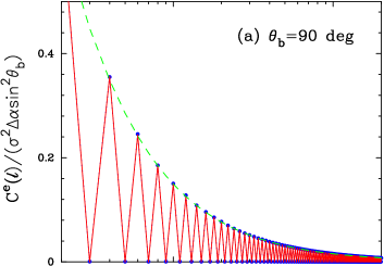
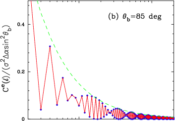
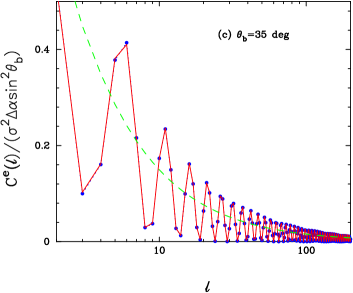
Figure 3: The power spectrum of destriping errors for ring tori with various values of $\theta_{b}$. In each figure the filled (blue) points show the results from numerical simulations and the solid (red) lines show the analytic expression of equation (18). The dot-dashed (green) line shows the simple analytic approximation of equation (21).

Defining the power spectrum of the error map as

$$\tilde{C}^{e}_{\ell}={1\over(2\ell+1)}\sum_{m}\langle a^{e}_{\ell m}a^{e*}_{\ell m},\rangle$$ (16)

(where the tilde on $\tilde{C}^{e}$ signifies that the power spectrum is computed from the $a^{e}_{lm}$ coefficients computed on the incomplete sky if $\theta_{b}\neq\pi/2$) and using the relation

$$\sum_{m}d^{\ell}_{m^{\prime}m}(\pi/2)d^{\ell}_{m^{\prime\prime}m}(\pi/2)=\delta_{m^{\prime}m^{\prime\prime}},$$ (17)

we find

$$\tilde{C}^{e}_{\ell}={2\pi\over(2\ell+1)}\sigma^{2}\Delta\alpha\sin^{2}\theta_{b}\sum_{m}|K_{\ell}^{m}(\cos\theta_{b})|^{2}.$$ (18)

For the special case $\theta_{b}=\pi/2$, the factor $|K_{\ell}^{m}|$ is proportional to $P_{\ell}^{m}(0)^{2}$ and so vanishes for odd values of $(\ell-m)$. Since $K_{\ell}^{m}$ is zero for odd values of $m$, it follows that $\tilde{C}^{e}_{\ell}=0$ for odd values of $\ell$. An alternative derivation of the $\tilde{C^{e}_{\ell}}$ for the special case $\theta_{b}=\pi/2$, (in which the spherical harmonic transform for each ring is evaluated in a coordinate system with the $z$-axis perpendicular to the spin axis) gives

$$\tilde{C}^{e}_{\ell}={1\over 2}\sigma^{2}\Delta\alpha I_{\ell},$$ (19a)

where

$$I_{\ell}=\left\{\begin{array}[]{ccc}-\int_{0}^{\pi}\theta\cos\theta P_{\ell}(\cos\theta)d\theta&\ell\;\;{\rm even},&\ell\neq 0\\ 0,&\ell\;\;{\rm odd}.&\end{array}\right.$$ (19d)

For large values of $\ell$ the integral in equation (19d) can be approximated by

$$-\int_{0}^{\pi}\theta\cos\theta P_{\ell}(\cos\theta)d\theta\approx\pi\int_{0}^{\infty}J_{0}((\ell+1/2)\theta)={\pi\over(\ell+1/2)},$$ (20)

hence

$$\tilde{C}^{e}_{\ell}\approx{\pi\over(2\ell+1)}\sigma^{2}\Delta\alpha,\qquad\ell\;\;{\rm even}.$$ (21)

Equation (21) is, in fact, an extremely good approximation (to within 2%) to the exact answers of equations (18) and (19a) for values of $\ell$ as small as $\ell=4$.

Some examples of the error power spectra for three values of $\theta_{b}$ are shown in Figure 3. For each value of $\theta_{b}$, $10^{4}$ simulations were generated each with $720$ rings assigned random offsets. The rings were then mapped on to the igloo pixelization scheme described in E04 with $0.25^{\circ}\times 0.25^{\circ}$ pixels simply by assigning the nearest map pixel to each ring pixel and averaging over all of the ring pixels assigned to any particular map pixel. The power spectra were computed from the igloo maps using using fast spherical transforms. As can be seen from Figure 2, the finite sizes of the ring and map pixels introduce some structure in the final error maps. Nevertheless, the mean power spectra for the error maps (shown by the points in Figure 3) agree perfectly with the analytic results of equation (18) which were derived in the continuum limit. Evidently, the effects of finite pixelisation and ring widths are negligible and hence the analytic model developed in this Section gives an extremely accurate representation of the destriping errors.

If the primordial fluctuations are Gaussian, the spherical harmonic coefficients will satisfy

$$\langle a^{e}_{\ell m}a^{e*}_{\ell^{\prime}m^{\prime}}\rangle=C_{\ell}\delta_{\ell\ell^{\prime}}\delta_{mm^{\prime}}.$$ (22)

The striping erros will, however, introduce correlations in the $a_{\ell m}$. From equation (15) it is straightforward to show that the correlations introduced by striping are given by

$$\langle a^{e}_{\ell m}a^{e*}_{\ell^{\prime}m^{\prime}}\rangle=2\pi\sigma^{2}\sin^{2}\theta_{b}\Delta\alpha\;\delta_{mm^{\prime}}\sum_{m_{1}m_{2}}K^{m_{1}}_{\ell}K^{m_{2}}_{\ell^{\prime}}d^{\ell}_{m_{1}m}(\pi/2)d^{\ell^{\prime}}_{m_{1}m^{\prime}}(\pi/2).$$ (23)

For the special case $\theta_{b}=\pi/2$, these correlations can be written as

$$\langle a^{e}_{\ell m}a^{e*}_{\ell^{\prime}m^{\prime}}\rangle=2\pi\sigma^{2}\Delta\alpha\;\delta_{mm^{\prime}}E^{m}_{\ell}E^{m^{\prime}}_{\ell^{\prime}}(1+(-1)^{m}),$$ (24a)

where

$$E^{m}_{\ell}=\int_{-1}^{1}A_{\ell}^{m}P^{m}_{\ell}(\mu)\;d\mu.$$ (24b)

If the vector $a^{e}_{\ell m}$ is ordered as $(m,\ell)$, (i.e. $(0,\ell_{\rm min}),\dots(0,\ell_{\rm max})$, $(1,\ell_{\rm min}),\dots(1,\ell_{\rm max})$, etc) the covariance matrix $\langle a^{e}_{\ell m}a^{e*}_{\ell^{\prime}m^{\prime}}\rangle$ will have a block diagonal structure. Figure 4 shows examples of these covariance matrices for the three scanning strategies discussed above. As we will show in the next Section, these off-diagonal correlations will be much smaller than the diagonal components for the parameters of a realistic experiment. However, since the departures from Gaussianity in most inflationary models are expected to be small (for a comprehensive review see Bartolo et al. 2004), residual map-making errors could prove problematic in testing for non-Gaussianity. For the remainder of this paper, we will concentrate on errors on estimates of the CMB power spectrum, though it is important to recognise that even if map-making errors can be shown to have a negligible effect on the power spectrum, they may be important for other statistical tests.

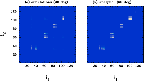
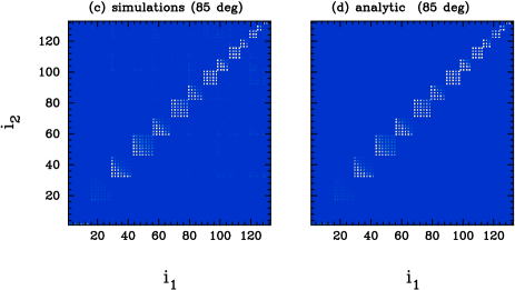
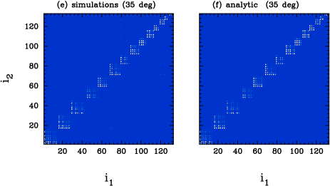
Figure 4: The covariance matrices for $\langle a^{e}_{\ell m}a^{e*}_{\ell^{\prime}m^{\prime}}\rangle$ for the simulations shown in Figure (3) compared to the analytic expression of equation (23). The indices $i_{1}$ and $i_{2}$ are ordered as $(m,\ell)$, (i.e. $(0,0),\dots(0,\ell_{\rm max})$, $(1,0),\dots(1,\ell_{\rm max})$, etc) with $m$ and $\ell$ running from $0$ to $10$.

4 Simulations with Realistic Noise

In this Section, we describe the results from a set of simulations with realistic ‘$1/f$’ noise (equation 1) with the parameters given in Table 1. As explained in Section 2, the resolution and sizes of the maps and ring sets were chosen so that large numbers of simulations could be run quickly while demonstrating the salient features of the map-making problem. As a further speed up, $1/f$-noise was generated by using an FFT for frequencies below $0.133\;{\rm Hz}$. Above this frequency the noise was assumed to be white, which has the additional advantage that the white noise can be added to ring pixels ‘on the fly’ so that it is never necessary to store a complete TOD in memory. A complete simulation, including noise generation, destriping and power spectrum estimation takes approximately $70$ seconds on an single $1.4\;$GHz Itanium 2 processor. Splitting the noise into a low frequency ‘$1/f$’ component and a high frequency white noise component has the additional advantage that the effects of low and high frequency noise on destriping can be investigated separately.

We have run two sets each of $250$ simulations for the two scanning strategies adopted for Figure 1, namely, $\theta_{b}=85^{\circ}$ with no precession and $\theta_{b}=85^{\circ}$ with a slow sinusoidal precession of $\pm 5^{\circ}$. In each case, we generated three ring-sets for each simulation: one with white noise only, one with low frequency ‘$1/f$’ noise only, and one using the sum of these two noise models. These ring-sets were passed through the destriping algorithm to produce three maps per simulation. The averaged power spectra for the two sets of simulations are plotted in Figure 5.

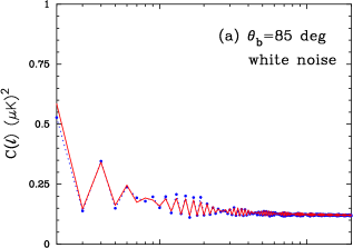
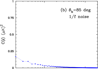
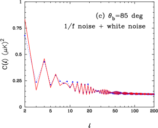
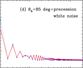
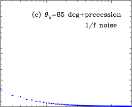
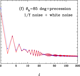
Figure 5: Averages over $250$ simulations of noise for a single detector with $\theta_{b}=85^{\circ}$ and no precession (Figures 5a, b, & c) and with a slow sinusoidal precession of $5^{\circ}$ amplitude as discussed in the text (Figures 5d, e & f). Filled circles in the upper panels (a & d) show residual errors after destriping assuming only uncorrelated white noise on the rings. Filled circles in the middle panels (b & e) show residual errors after destriping assuming only low frequency $1/f$ noise. Filled circles in the bottom panels (c & f) show residual errors including white noise and low frequency $1/f$ noise. The solid lines in the upper panels show the model for destriping errors plotted in Figure 3b together with the white noise level appropriate to the maps. The solid lines in the lower panels show the same destriping model renormalised to fit the simulations.

The upper panels in Figure 5 show the power spectra for the case of white noise only on the rings. This is the case that is closest to the analytic model of the previous Section. As expected, the analytic model of equation (18) summed with the appropriate constant white noise level, provides an excellent match to the simulations when proper allowance is made to calculate the effective ring width using the correlation functions of Figure 1. This is true even for the slow precession scanning strategy shown in Figure 5d. The main effect of a the slow precession is to fill in the coverage gaps at the eclipic poles, but the ring pattern is so close to a perfect ring torus that the residual striping errors produce a nearly identical effect on the power spectrum.

Figures 5b and 5e show the residual striping errors when only low frequency ‘$1/f$’ noise is included. These errors arise primarily from residual gradients on the rings and so their amplitude depends on the knee frequency. Had we adopted a knee frequency much smaller than the spin frequency, these errors would have had a much lower amplitude. Nevertheless, even for the parameters adopted here, the amplitude of these errors is considerable smaller than the errors caused by the dispersions in the ring offsets. Notice that these errors also decay roughly as $1/\ell$, as for the error power spectra for pure white noise. As mentioned earlier, Delabrouille (1998) and Keihänen et al. (2003) have explored fitting low order functions for each ring during destriping, rather than a single offset $\epsilon_{k}$. The results are mixed and in fact Keihänen et al. (2003) find that including more parameters actually produces larger power spectrum errors than simply fitting constant offsets. This is not suprising because the errors on the individual crossing points are dominated by the white noise. If the white noise level is high, and the knee frequency is low, there may not be enough crossing points to determine more than a single constant offset per ring with any precision.

The points in the lower panels in Figure 5 show the errors for the full noise model. These are just the sum of the white noise and ‘$1/f$’ errors. The theoretical models, plotted as the solid lines, are simply equation (18) rescaled to provide a good match to the simulations, summed with the appropriate constant white noise level. These provide an excellent match to the simulation results. The general shape of the power spectrum errors $C^{e}_{\ell}$ plotted in Figures 5c and 5f is well known from previous numerical work on destriping (Delabrouille 1998; Maino et al. 1999; et al. 2000; Keihänen et al. 2003). However, the results presented here explain why the errors have this particular form and how they depend on the parameters of the experiment.

Finally, in Figure 6 we illustrate the effects of ‘$1/f$’ noise on a simulated map of the CMB sky for the scanning strategy with a slow sinusoidal precession. Figure 6a shows the power spectra of the input map, the destriped map and for the difference map. The power spectrum of the difference map is shown on a greatly expanded scale in Figure 6b, together with the analytic model plotted in Figure 5f. Figure 6c shows the differences between the power spectra of the input and output maps but with the white noise level subtracted, again plotted on an expanded scale. The solid lines show the expected errors

$$\langle(\Delta C_{\ell})^{2}\rangle^{1/2}=\sqrt{{(2(C^{e}_{\ell})^{2}+4C^{e}_{\ell}C_{\ell})\over(2\ell+1)}},$$ (25)

using the error model of Figure 5f. The dotted lines in this Figure show the expected error from white noise alone. Notice that pure white noise is an excellent approximation to the errors for $\ell\lower 2.15277pt\hbox{$\;\buildrel>\over{\sim}\;$}10$ and that even at low multipoles the destriping errors are much smaller than the cosmic variance $\langle\Delta C_{\ell}^{2}\rangle=2C_{\ell}^{2}/(2\ell+1)$. For example, the error in the quadrupole amplitude for this realisation is $\Delta T_{2}^{2}=\ell(\ell+1)\Delta C_{2}/2\pi=10.4\;{\rm\mu K^{2}}$, compared to the expected cosmic variance of $\Delta T_{2}^{2}=717.8\;{\rm\mu K^{2}}$. Compared to the cosmic variance, the destriping errors at low multipoles can be ignored. Furthermore, errors of this magnitude are much smaller than the errors of $50$-$100\;{\rm\mu K}^{2}$ expected from inaccurate subtraction of the Galaxy (cf the discussion of the effects of Galactic subtraction on the low multipoles measured by WMAP, Bennet et al. 2003; Slosar and Seljak 2004).

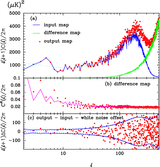
Figure 6: The top panel (a) shows the power spectrum of the input map (solid line) and the power spectrum of the destriped map (filled circles). The dashed line shows the power spectrum of the fiducial $\Lambda$CDM model used to generate the input map. The power spectrum of the difference (noise) map is also shown. The middle panel (b) shows the power spectrum of the difference map on an expanded scale (filled circles) together with the error model shown in Figure 5f. The filled circles in the lower panel (c) show the differences between the power spectrum of the destriped map. after subtracting the constant white noise level, and the power spectrum of the input map. The solid lines show the dispersion expected from equation (25) using the error model plotted in Figure (6b). The dashed lines show the disersion expected from white noise alone.

5 Conclusions

In this paper, we have presented an analytic analysis of the effects of destriping errors on the CMB power spectrum for various scanning strategies. Destriping errors produce a characteristic error power spectrum of the form shown in Figure 3 which decays roughly as $1/\ell$. The amplitude of the error power spectrum is determined by the number of intersections in the ring set which depends on the scanning strategy. In agreement with Stompor and White (2003), and with earlier numerical work, there are so many interconnections in a Planck-like scanning strategy that the destriping errors should be small. Maps from Planck will therefore be dominated by white noise, underneath which there will be low amplitude correlated noise associated with striping. Nevertheless, the low amplitude errors from striping introduce a characteristic block-diagonal structure in the covariance matrix for the $a_{\ell m}$. These could confuse searches for small amplitude physical effects, such as non-Gaussian features of the CMB signal.

The implications of our analysis for the application of a hybrid power spectrum estimator to Planck-like data are fairly self-evident. Since the noise can be very accurately approximated as white for multipoles $\ell\lower 2.15277pt\hbox{$\;\buildrel>\over{\sim}\;$}50$, the combination of a number of pseudo-$C_{\ell}$ estimators with different pixel weighting schemes as in E04 should give a close to optimal estimate of the power spectrum at high multipoles. At low multipoles, an estimate of $C_{\ell}$ can be found by applying a quadratic maximum likelihood (QML) estimator (Tegmark 1997c) to a low resolution map. This providesa close to optimal estimate of the power spectrum at low multipoles, taking into account of masked regions of the sky, and returns an estimate of the covariance matrix $\langle C_{\ell}C_{\ell}^{\prime}\rangle$ that . For the QML estimates, it should be an excellent approximation simply to neglect destriping errors, since these are likely to be negligible compared to the cosmic variance. If necessary, destriping errors can be taken into account in the QML estimates, and folded into the covariance matrix, by computing the full pixel-noise covariance matrix on a low resolution map using an optimal map making algorithm.

Finally, this analysis has some implications for optimal map making algorithms. The maximum likelihood map $\tilde{\bf m}$ is given by the well-known expression

$$\tilde{\bf m}=({\bf P}^{T}{\bf N}^{-1}{\bf P})^{-1}{\bf P}^{T}{\bf N}^{-1}{\bf t},$$ (26)

where ${\bf N}$ is the noise covariance matrix $N_{ij}=\langle n_{i}n_{j}\rangle$. Since ${\bf N}$ is symmetric, it can be written as

$${\bf N}={\bf W}{\bf\Lambda}{\bf W}^{T},$$ (27)

where ${\bf W}$ is orthogonal and ${\bf\Lambda}$ is diagonal. The matrix ${\bf W}^{T}$ is a ‘prewhitening filter’, since the noise matrix of the vector ${\bf n}^{\prime}={\bf W}^{T}{\bf t}$ is diagonal. In terms of the prewhitened time-stream, equation (26) can be written as,

$${\bf P}^{T}{\bf W}{\bf\Lambda}^{-1}{\bf W}^{T}{\bf P}\tilde{\bf m}={\bf P}^{T}{\bf W}{\bf\Lambda}^{-1}{\bf W}^{T}{\bf t}.$$ (28)

Now consider equation (28) applied to a TOD consisting of repeated scans of a single ring with stationary noise of an arbitrary power spectral shape. If edge effects are ignored then the components of ${\bf\Lambda}$ will be identical, in which case the solution of (28) is obviously the average of $t$ over the rings (equation 4). The rhs of equation (28) effectively filters the TOD, but this is undone by the lhs to return the average of the signal over the rings.

Now consider a TOD consisting of a set of rings as in the Planck-like scanning strategies considered in this paper. The maximum likelihood map will differ from a simple average over rings because the rings cross. Thus optimal map making performs destriping by comparing the crossing points of the TOD. However, since the noise on a single ring is dominated by white noise, optimal map making cannot reduce the errors much below the ‘irreducible’ white noise errors shown in Figures 5a and 5d. Optimal map making can, in principle, reduce the map making errors associated with ‘$1/f$’ noise (cf Figures 5b and 5e) if the knee frequency is significantly greater than the spin frequency, but even in this case, the ability to reduce these errors will be limited by the white noise on a ring. These arguments suggest that for a Planck-like scanning strategy, simple destriping algorithms will be very close to optimal, and may actually be preferable to optimal algorithms because of their speed and because they require fewer assumptions about the noise. Optimal algorithms are only optimal if the noise model is accurate. In practice, with realistic non-stationary noise, simple destriping may perform just as well and conceivably better than an optimal algorithm.

Acknowledgements: I thank members of CITA for their hospitality during a visit where this work was begun. I am especially grateful to Mark Ashdown, Dick Bond, Anthony Challinor and Floor van Leeuwen for helpful discussions.

References

- [BKMR2004] Bartolo N., Komatsu E., Matarrese S., Riotto A., 2004, submitted to Physics Reports. astro-ph/0406398.
- [Betal032003] Bennett, C. et al., 2003, ApJS, 148, 1.
- [BS931993] Brink D.M., Satchler G.R,. 1993, Angular Momentum, third edition, Oxford University Press, Oxford.
- [BFJS2001] Borrill J., Ferreira P. G., Jaffe A. H., Stompor R., 2001, In ‘Mining the Sky’, Proceedings of the MPA/ESO/MPE Workshop, Edited by A. J. Banday, S. Zaroubi, and M.Bartelmann. Springer-Verlag, Heidelberg, p403.
- [BMMDMBM971997] Burigana C., Malaspina M., Mandolesi N., Danese L., Maino D., Bersanelli M., Maltoni M., 1997, Internal Report ITESRE. astro-ph/9906360.
- [D981998] Delabrouille, J., 1998, A&A Suppl. Ser., 127, 555.
- [DKP012001] Doré O., Teyssier R., Bouchet F.R., Vibert D., Prunet S., 2001, A&A, 374, 358.
- [E03b2003] Efstathiou G., 2004, MNRAS, 439, 603.
- [BP861986] Groth E.J., Peebles P.J.E., 1986, ApJ, 310, 507.
- [Hetal032003] Hinshaw G. et al., 2003, ApJS, 148, 63.
- [KKPMB032003] Keihänen E., Kurki-Suonio H., Poutanen T., Maino, D., Burigana C., 2003, submitted to A&A. astro-ph/0304411.
- [Metal991999] Maino D., et al., 1999, A&A Suppl. Ser., 140, 383.
- [MES961996] Maddox S.J., Efstathiou G., Sutherland W., 1996, MNRAS, 283, 1227.
- [NdeGGV011997] Natoli P., de Gasperis G., Gheller C., Vittorio N., 2001, A&A, 372, 346.
- [PMKKH042004] Poutanen T., Maino, D., Kurki-Suonio H., Keihänen E., Hivon E., 2004, submitted to MNRAS. astro-ph/0404134.
- [RKACDK002000] Revenu B., Kim A., Ansari R., Couchot F., Delabrouille J., Kaplan J., 2000, A&AS, 142, 499.
- [SS042004] Slosar A., Seljak U., 2004, submitted to PRD, astro-ph/0404567.
- [Setal032003] Spergel D.N. et al., 2003, ApJS, 148, 175.
- [SW42004] Stompor R., White M., 2004, A&A, 419, 783.
- [T97a1997] Tegmark M., 1997a, ApJL, 480, L87.
- [T97b1997] Tegmark M., 1997b, PRD, 56, 4514.
- [T97c1997] Tegmark M., 1997c, PRD, 55, 5895.
- [T031997] Tuovinen J., 2003, Planck Newsletter Number 4., p7. (http://www.rssd.esa.int/SA/PLANCK/docs/Newsletters/PlanckNewsletter4.pdf)
- [VMK881988] Varshalovich, D.A., Moskalev A.N., Khersonskii V.K., 1988, Quantum Theory of Angular Momentum, World Scientific, Singapore.
- [vLetal2002] van Leeuwen F., et al., 2002, MNRAS, 331, 975.
- [W961996] Wright E.L., 1996, astro-ph/9612006.
- [WHB961996] Wright E.L., Hinshaw G., Bennett C.L., 1996, ApJ, 458, L53.