On the importance of the few most massive stars:
the ionizing cluster of NGC 588

We present the results of a double analysis of the ionizing cluster in NGC 588, a giant HII region (GHR) in the outskirts of the nearby galaxy M33. For this purpose, we obtained ground based long-slit spectroscopy and combined it with archival ground based and space borne imaging and spectroscopy, in the wavelength range 1100–9800 Å. A first modeling of the cluster was performed using integrated properties, such as the spectral energy distribution (SED), broad band colors, nebular emission H$\beta$ equivalent width, the main ultraviolet resonance lines, and the presence of Wolf-Rayet star features. By applying standard assumptions about the initial mass function (IMF), we were unable to fit satisfactorily these observational data. This contradictory result led us to carry out a second modeling, based on a resolved photometric analysis of individual stars in Hubble Space Telescope (HST) images, by means of finding the best fit isochrone in color-magnitude diagrams (CMD), and assigning a theoretical SED to each individual star. The overall SED of the cluster, obtained by integrating the individual stellar SEDs, is found to fit better the observed SED than the best solution found through the integrated first analysis, but at a significantly later stage of evolution of the cluster of 4.2 Myr, as obtained from the best fit to the CMD. A comparative analysis of both methods traces the different results to the effects of statistical fluctuations in the upper end of the IMF, which are significant in NGC 588, with a computed cluster mass of 5600 M_☉, as predicted by Cerviño et al. (2002). We discuss the results in terms of the strong influence of the few most massive stars, six in the case of NGC 588, that dominate the overall SED and, in particular, the ionizing far ultraviolet range beyond the Lyman limit.

1 Introduction

Despite their small number in comparison with Sun-like stars, massive stars are most influential in their host galaxies. They are responsible for the release in the interstellar medium of most of the mechanical energy, metals such as oxygen, neon, sulfur, etc. and possibly carbon, and hard radiation. However, their formation is still poorly understood. It is generally admitted that massive stars form mainly in instantaneous starbursts, with a power-law initial mass function (IMF) with universal slope (e.g., Massey 2003), although Scalo (1998) estimates that this slope may comprise a natural scatter of a few tenths between different clusters. Most massive stars are observed and studied in very massive clusters embedded in giant HII regions (GHRs), in which the ionized gas provides information on the intensity of the (unobservable) stellar Lyman continuum, via the equivalent width of the nebular H$\beta$ line. Inversely, modeling accurately a GHR from its emission spectrum requires a good knowledge of the ionizing spectrum of its source, which is one of the elements that control the temperature and ionization state of the gas. This ionizing spectrum is unobservable, and can only be derived from a model of the stellar source.

The stellar content of a GHR can be determined in two ways: either by observing the individual stars, or making assumptions regarding the distribution of their initial masses. The first solution can be used to study the cluster itself via color-magnitude diagrams (CMDs, e.g. Malamuth et al. 1996) or to synthesize an ionizing spectrum to be input to photoionization models (Relaño et al. 2002). However, such a procedure requires quite high resolution and sensitivity for extragalactic objects, which can in general be reached only with the HST. In the vast majority of other cases, only integrated properties of the cluster can be used, and an IMF, generally a continuous power law, must be supposed. Nevertheless, Cerviño et al. (2002) showed that if the total initial mass of a cluster is less than $\sim 10^{4}$ M_☉, statistical fluctuations around the mean IMF can strongly affect the main diagnostics of the cluster, like the H$\beta$ equivalent width $W({\rm H}\beta)$, as well as the determined ionizing spectrum (see also Cerviño et al. 2003). The effects of these fluctuations need to be tested with observational data.

In this article, we show that the cluster embedded in NGC 588 nicely illustrates the issue of IMF statistical sampling. Section 2 describes all the data sets used, spectroscopic and photometric, ground based and space borne, either obtained by us or retrieved from different archives. Further data processing is detailed in Section 3. Section 4 describes a first modeling of the star cluster, using a “classical” approach, aimed at fitting its integrated spectral properties with a model assuming an analytical IMF. In Section 5 we introduce the importance of modeling the effects of statistical fluctuations. In Section 6, we measure the fluxes of the individual stars detected in HST images, and use the photometric results to analyze the stellar content of the cluster, by assigning a model SED to each individual star. The results from the two methods of modeling are significantly discrepant, and in Section 7 we explore how this discrepancy can be attributed to the role of the few most massive stars, whose number is heavily affected by statistical fluctuations in the case of the low mass cluster ionizing NGC 588.

2 Observational data and standard reduction

We have performed ground based optical spectroscopic observations of NGC 588 and have retrieved the available archival spectroscopic and imaging data sets from the Hubble Space Telescope (HST), the International Ultraviolet Explorer (IUE), and the Isaac Newton Group (ING). Table 1 contains a summary of the different data sets used in this study.

Table 1: Journal of Observations.

Spectroscopy
CAHA (PA=121∘, width=1.2$\arcsec$, 1998-08-27/28)
range: $\lambda$ (Å)	$\Delta\lambda$ (Å/pixel)	exposure (s)
B : 3595–5225	0.81	$4\times 1800$
R1: 5505–7695	1.08	$2\times 1800$
R2: 7605–9805	1.08	$2\times 1800$
HST/STIS (PA=-154∘, width=0.2$\arcsec$, 2000-07-13)
range (Å)	exposure (s)	data set
1447–3305	1440	O5CO05010
1075–1775	480	O5CO05020
1075–1775	2820	O5CO05030
IUE (PA=102∘, large aperture, 1980-10-03)
range	exposure (s)	data ID
1150–1980	18000	SWP10273
1850–3350	18000	LWR08943
Imaging
HST/WFPC2 (Proposal: 5384, 1994-10-29)
Filter	exposure (s)	data set
F170W	$2\times 350$	U2C60701T/702T
F336W	$2\times 160$	U2C60703T/704T
F439W	$2\times 180$	U2C60801T/802T
F547M	$2\times 100$	U2C60803T/804T
JKT (1990-08-20/21)
Band	Filter	exposure (s)
H$\beta$	4861/54	$2\times 1800$
H$\alpha$	6563/53	1800
H$\alpha$ continuum	6834/51	1300

2.1 Optical spectra

Optical spectra were obtained in 1998 August 27/28 with the 3.5m telescope at the Centro Astronómico Hispano Alemán (CAHA, Calar Alto, Almería). The observations were made with the dual beam TWIN spectrograph, using the blue and red arms simultaneously, with the beam-splitter at 5500 Å, and SITe-CCDs of $2000\times 800$ 15$\mu$ pixels. Four exposures of 1800 s each were taken with the blue arm in the range 3595–5225 Å, while two 1800 s exposures in the range 5505–7695 Å and two 1800 s in the range 7605–9805 Å were taken in the red arm (hereafter, the B, R1 and R2 ranges, respectively). The gratings T7 in the blue and T4 in the red give dispersions of 0.81 and 1.08 Å/pixel in second and first spectral order, respectively. A slit, oriented at PA$=121^{\circ}$ (Fig. 1), of size $240\arcsec\times(1.2\pm 0.2)\arcsec$ provided a spectral resolution, similar in both arms, of FWHM$\sim 2$ Å, as measured in the background sky emission lines.

These spectra were reduced, following the standard procedure, by means of the IRAF package noao.twodspec.longslit. Photometric calibration was achieved by means of three standard stars, BD+28~4211, G191-B2B and GD71, observed during the same night and setup, but through a wide slit. We estimated the resulting photometric accuracy to be 3% in color, except for the $\lambda<4000$ Å range (residuals are $\sim 5$% intrinsic to this range, $\sim 15$% with respect to the global spectrum), where the sensitivity curve drops, and for the $\lambda>8000$ Å range (accuracy $\sim 30$%), which is strongly affected by telluric absorption bands. The absolute photometric level was determined with $\sim 10$% accuracy. The reduction included the subtraction of the background measured in the slit aside the nebula, and consequently, the light of the underlying stellar population of M33 was removed from our spectra.

2.2 IUE spectra

We retrieved two spectra from the final archive IUE Newly Extracted Spectra (INES: Rodríguez-Pascual et al. 1999; Cassatella et al. 2000; González-Riestra et al. 2000). The SWP and LWR spectra cover a total range of 1150–3350 Å, and were obtained in the low-resolution mode ($\sim$5 Å) through the large aperture ($9.5\arcsec\times 22\arcsec$; cf. Fig. 1).

The two IUE spectra were retrieved from the archive in two formats: the integrated, fully calibrated spectra, and the two-dimensional frames, linearized in wavelength and position. The slit position and mean angular resolution were known with an accuracy of a few arcseconds, a scale comparable to that of the densest spatial structures of the cluster, and we re-determined them more accurately following the procedure detailed in § 3.2. Furthermore, due to significant uncertainties in the photometry of the LWR spectrum, we limited our use of IUE data to the SWP spectrum.

2.3 Ground-based images

We downloaded a set of images of NGC 588 from the Isaac Newton Group of telescopes archive. These images were taken with the 1m Jacobus Kapteyn Telescope (JKT) at the Observatorio del Roque de los Muchachos (La Palma), through the filters H$\alpha$+[NII], H$\beta$, and a continuum narrow band filter close to H$\alpha$.

Line emission only images were obtained by subtracting a version of the continuum image scaled with stars common to the three filter images. Then, we divided the H$\alpha$+[NII] image by the H$\beta$ one, thus establishing an extinction map of the nebula (the intensity of the [NII] $\lambda$6548+6583 doublet being small compared to H$\alpha$, according to our spectra). We observed no significant gradient of extinction across the object. We also registered the images with respect to the HST images, in order to locate the slits of the different spectrographs over the nebula (Fig. 2).

2.4 HST images

We retrieved five pairs of WFPC2 images from the HST archive, taken through the filters F547M, F439W, F336W, F170W and F469N. The images were calibrated with the on-the-fly calibration system. Each pair of exposures within a filter was combined with crrej in order to perform cosmic ray rejection.

The images were corrected for filter contamination, as recommended by McMaster & Whitmore (2002). These corrections consisted of increasing the measured fluxes by 0.044 magnitude for filter F170W, 0.006, for F336W and 0.002, for F439W. We also accounted for charge-transfer efficiency loss (Whitmore et al. 1999). This was necessary because of the low background levels in our images ($\sim$0.3 to 0.5 DN). In the case of individual stellar photometry (Section 6.1), we applied directly the formulae of Whitmore et al. (1999) to correct the number of counts in each star. In the case of integrated fluxes (Section 4), we used an average correction for each filter based on the rough locus of the cluster on the images ($X\sim 400$ and $Y\sim 450$) and on the approximate counts found in the stars that dominate the total cluster flux. These corrections are of 0.037, 0.035, 0.036 and 0.044 magnitude for filters F547M, F439W, F336W and F170W, respectively. We neglected the effects of geometric distortions, because the cluster is close to the center of the images, and the photometric effects of these distortions are small compared to other errors.

We computed the barycentric wavelengths of the filters. For this, we multiplied the spectral response of each filter by a few SEDs characteristic of young OB associations, and calculated the corresponding barycentric wavelengths. For F547M, F439W, F336W, F170W and F469N, we respectively found 5470, 4300, 3330, 1740 and 4690 Å. These wavelengths were then used to compute the values of the extinction laws to be applied.

2.5 STIS spectra

The HST archive contains three STIS spectra through NGC 588, covering the two wavelength ranges 1447–3305 Å (with the grating G230L) and 1075-1775 Å (with the grating G140L), the two spectra covering the latter range having a resolution of $\sim$1.5 Å. We retrieved these spectra with on-the-fly calibration. The spectra pass only through the brightest star of NGC 588 (Fig. 1), and we used them to identify its spectral class (Section 6.2 below).

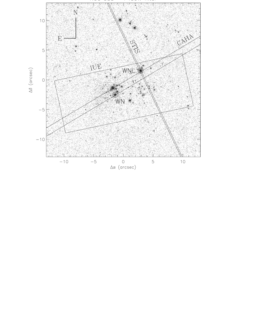
Figure 1: HST image of NGC 588 in filter F439W and the spectral slits. The peculiar stars (WNL, WN) are discussed in Section 6.

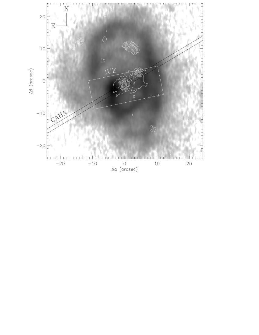
Figure 2: H$\alpha$+[NII] image of NGC 588 and CAHA and IUE slits. The contours represent the H$\alpha$ continuum.

3 Additional spectroscopic and photometric processing

3.1 Nebular extinction

Once the spectra were reduced, we performed a self-consistent procedure to deredden the nebular lines, based on the Balmer lines H$\alpha$ through H$\delta$. First, the emission line fluxes were corrected for foreground Galactic extinction, which amounts to $E_{B-V}=0.045$ (Burstein & Heiles 1984), the Galactic law being here the ensemble of the Seaton (1979) ultraviolet law and of the optical law of Nandy et al. (1975) (as shown in Seaton’s paper). Then a reddening law was fitted to the thus corrected Balmer decrement, taking into account the photometric and measurement errors of these emission lines. This process was performed for each spatial increment along the slit independently, thus obtaining the reddening along the slit. The residuals from the actual line ratios to the fitted law were then plotted along the slit, giving statistical fluctuations around a mean offset value (due to a small residual photometric calibration) except at those locations where the underlying stellar population has a significant contribution of Balmer lines in absorption. The equivalent width of the lines at these locations was thus computed and the correction applied to the intensity of the emission lines, then computing the corrected value of reddening. Assuming the LMC extinction law (Howarth 1983), a priori adequate due to the metallicity of the object (Vílchez et al. 1988), we derived an $E_{B-V}$ curve along the slit, and found it to be almost constant, with a value of $0.11\pm 0.02$ around the stellar cluster. This result is virtually independent of the selected extinction law, since different laws predict nearly the same relative extinctions within the H$\delta$–H$\alpha$ wavelength range.

3.2 Spatial registration between spectra and images

We have registered precisely the position of the CAHA slit with respect to the HST images. This is achieved by convolving the HST images with the atmospheric point spread function (PSF) at the time of the ground based observations, and comparing the spatial flux distributions. In order to compute the atmospheric PSF we modeled the spatial flux distribution of a point source in the 2D spectral frames in the following way. We assumed the atmospheric PSF to be a Moffat (1969) function, $h(r)=(1+(r/R_{c})^{2})^{-\beta}$. We selected a standard star observed just before NGC 588, and examined its profile along the slit around 4400 Å. This profile was clearly asymmetrical, indicating image distortion inside the spectrograph. We found that the observed star profile is very well reproduced by a model of the form $H(x)=\sum_{i=1}^{3}a_{i}M(x-c_{i})$, where $x$ is the spatial increment variable, $c_{i}$ the spatial location of the peak of each component and $a_{i}$ its weight, and $M(x)$ is the Moffat PSF integrated across the slit width. Thus, we assumed that the signal of the observed object was convolved by a Moffat function determined by turbulence, truncated by the slit, and split into three components within the spectrograph, before hitting the detector. The same analysis near 6600 Å and 8700 Å led to similar models. Once the PSF model was established, we proceeded as follows.

The blue 2D spectral frame was multiplied by the response of the HST filter F439W and the result integrated along the wavelength axis; in this way we obtained from the spectral frames the spatial flux distribution of NGC 588 through the HST filter F439W. Then, we applied our image degradation model to the HST image for different values of the Moffat parameters $R_{c}$ and $\beta$ (that tend to vary with time), placed a synthetic slit on the blurred image, and extracted the profile integrated across the slit. $R_{c}$, $\beta$ and the central position of the slit were fit by maximizing the correlation between the profiles extracted from the spectrum and from the image. We found $R_{c}\approx 1.1\arcsec$ and $\beta\approx 1.5$, corresponding to a seeing of FWHM$\sim 1.6$ arcsec. The PSF and the slit position were used to calculate the aperture throughputs used in Section 4 and 6.

We also used the two-dimensional frames and the F170W HST/WFPC2 image to determine accurately the slit position and angular resolution of the IUE data, assuming a Gaussian PSF and using the same technique as for the optical spectra. The resulting correlation is very good for a FWHM of 6.4$\arcsec$, with however a strong photometric mismatch between the data: the IUE flux integrated within the F170W band was found to be higher than the HST one by a factor 1.41. This mismatch between IUE and HST absolute calibrations has been found also for NGC 604 (González Delgado & Pérez 2000). HST absolute photometry is accurate to a few %, so we decided not to correct the HST image, but to divide the IUE spectra by the factor 1.41.

3.3 Nebular continuum subtraction

To analyze the spectral properties of the cluster itself, we removed the nebular continuum from our spectra. For this, we calculated it according to Osterbrock (1974), including the HI free-free, free-bound and two-photon components as well as the HeI free-free and free-bound emissions, assuming a gas temperature of 11000 K (Vílchez et al. 1988); we reddened the computed nebular continuum to match the observations, normalized it with the nebular H$\beta$ emission line intensity in the spatial zone of the optical slit selected to study the cluster (knowing the H$\beta$ equivalent width with respect to the nebular continuum), and removed it.

3.4 Aperture throughput correction

Once the optical and UV slit positions and angular PSFs were determined (see Section 3.2), we calculated the aperture throughputs of the slits for the whole cluster, i.e. the fraction of light transmitted by these slits. For this, we computed the sky background of each image by averaging, at a given position, the pixels contained in a rectangular box and close enough to the median value of this box. The resulting map of the sky and of the nebula was removed from the original in order to keep only the stellar signal. The remaining stellar images were then convolved by the optical or UV PSFs, and in each band, we compared the total flux of the cluster to the one entering the slit. In optical, the aperture throughputs were found to be independent of the band (F170W, F336W, F439W or F547M), and we retained a mean value of 0.169 for a slit width of 1.2”, valid in the whole optical range. This throughput was proportional to the chosen slit width, known to $\approx$20% accuracy. The uncertainty on the PSF led to an uncertainty of 10% on the throughput. For the IUE spectra, we found a throughput of 0.83 in the F170W filter. This means that we had to divide the CAHA spectra by 0.169, and the IUE spectra, by 0.83, in order to obtain the integrated spectrum of the whole cluster. We also calculated the aperture throughputs for nebular emission: 0.062 for the optical spectra, and 0.44 for IUE data.

4 Integrated canonical modeling of the cluster

The cluster was first modeled in the classical way, i.e. as a stellar population whose IMF is rigorously a continuous power law $dN/dm\propto m^{-\alpha}$, $m_{\rm low}\leq m\leq m_{\rm up}$. Assuming instantaneous star formation, we used Starburst99 (Leitherer et al. 1999), with $m_{\rm low}=1$ M_☉, making use of standard mass-loss evolutionary tracks at metallicities Z=0.004 (Charbonnel et al. 1993) and Z=0.008 (Schaerer et al. 1993), close to the metallicity of the gas (Vílchez et al. 1988) (the solar value is here Z=0.02). We selected the atmosphere models of Lejeune et al. (1997), Hillier & Miller (1998) and Pauldrach et al. (2001), the latter two ones having been compiled by Smith et al. (2002). The age $\tau$ of the cluster, its metallicity Z, and the IMF slope $\alpha$ and upper limit $m_{\rm up}$ were constrained with observables available for the cluster as a whole. These are: i) the UV and optical colors, integrated over the entire cluster; ii) the H$\beta$ equivalent width $W({\rm H}\beta)$ measured over the whole object (nebula and cluster); iii) the profiles of the UV stellar lines present in the IUE spectrum; iv) the presence or absence of the main Wolf-Rayet (WR) emission lines in the optical SED.

4.1 SED colors and derived extinction

The SED colors were used to determine the amount and the law of extinction of the stellar flux. Indeed, the color excess $E_{B-V}$ derived from the Balmer lines of a nebula has been found not to apply systematically to its ionizing source (e.g., Mas-Hesse & Kunth 1999). Furthermore, whereas different extinction laws generally do not differ significantly from each other in the optical range and cannot be discriminated by the use of the nebular Balmer lines, they strongly vary in the UV counterpart. Fortunately, the intrinsic UV and optical colors of an OB association little depend on the age and IMF of the latter, and can be used to characterize the extinction, provided that one knows approximately the main characteristics of this association. Mas-Hesse & Kunth (1999) found an age of 2.8 Myr for a very flat IMF ($\alpha=1$) with an upper mass cutoff of 120 M_☉, for the cluster of NGC 588. We computed SEDs for a range of ages, IMF slopes and upper mass cutoffs around these values, and calculated the corresponding fluxes in the four bands F547M, F439W, F336W and F170W. Then, the colors of the cluster were measured on the HST images cleared of their diffuse background. Table 2 shows the measured colors and some model outputs. The differences of color between the observations and the models were attributed to interstellar reddening. We tested three extinction laws: Galactic (Seaton 1979; Nandy et al. 1975), LMC (Howarth 1983) and SMC (Prévot et al. 1984; Bouchet et al. 1985), whose values at the barycentric wavelengths of the bands are summarized in Table 2. For any set of model colors, the best fit was obtained with the SMC law and $E_{B-V}=0.08\pm 0.04$ (the error bar includes the uncertainties in the observational data and the spread in the theoretical colors). This value is compatible with the amount of extinction derived from the nebular Balmer lines, meaning that there is no indication of differential extinction between the stellar and the nebular fluxes. Since the nebular value, $E_{B-V}=0.11\pm 0.02$, was determined more accurately, we have also adopted it for the cluster in the following. Considering these results and the 800 kpc distance of M33 (Lee et al. 2002), we derived the cluster luminosity in the F439W band: 4.71$\times$10³⁵ erg s^-1 Å^-1.

Filter	F547M	F439W	F336W	F170W
$\lambda$ (Å)	5470	4300	3330	1740
Obs. $M_{547}-M_{\lambda}$	0.00	0.84	1.48	3.03
	$\pm$0.03	$\pm$0.03	$\pm$0.04	$\pm$0.05
$M_{547}-M_{\lambda}$ (a)	0.00	0.96	1.85	4.10
$M_{547}-M_{\lambda}$ (b)	0.00	0.87	1.49	3.22
$M_{547}-M_{\lambda}$ (c)	0.00	0.82	1.19	2.94
$f(\lambda)$ (Galactic)	3.21	4.18	5.06	7.80
$f(\lambda)$ (LMC)	3.10	4.13	5.37	9.25
$f(\lambda)$ (SMC)	2.72	3.65	4.65	10.51

Table 2: Observed and model colors with filter F547M as the zero point. The observed colors are here corrected for foreground Galactic extinction. The three models (a), (b) and (c) shown here stand for $m_{\rm up}=120$ M_☉, Z=0.004, and respectively, $\alpha=1$, 1 and 2.35 and $\tau=$2, 3 and 4 Myr. We also show the three tested extinction laws in the form $f(\lambda)=A(\lambda)/E_{B-V}$. The color differences $\Delta(M_{y}-M_{\lambda})$ between the observations and a given model were to be well fit by a function of the form $a+E_{B-V}f(\lambda)$ for the tested extinction law to be accepted.

4.2 H$\beta$ equivalent width

This quantity is often used in modeling of massive stellar populations, as a way to characterize the ratio of the ionizing photon rate to the optical continuum. It is mainly sensitive to the global distribution of effective temperatures of the stars, although it also depends on the fraction of the ionizing flux absorbed by the nebular gas. Since this fraction is a priori unknown, we decided only to require the model to predict $W({\rm H}\beta)$ greater than or equal to the observed value.

The value of $W({\rm H}\beta)$ used here is the ratio of the total nebular H$\beta$ flux to the stellar H$\beta$ continuum integrated over the cluster. The integrated values of these two quantities were obtained by dividing the values measured in the blue CAHA spectrum (cleared of the nebular continuum; see Section 3.3) by the aperture throughputs of the optical slit for the nebular gas and for the stellar continuum (Section 3.4). This estimate of $W({\rm H}\beta)$ is affected by the error in the nebular-to-stellar ratio of the two aperture throughputs, evaluated to $\approx$10%. We found $W({\rm H}\beta)=330\pm 30$ Å.

4.3 UV lines

The UV lines that form in the atmospheres of massive stars were studied by Sekiguchi & Anderson (1987a). They showed the correlation existing between the shapes and intensities of the SiIV $\lambda$1400 and CIV $\lambda$1550 lines and the spectral type and luminosity class of early-type stars. The use of these two lines and, in some cases, the HeII $\lambda$1640 line, can be a good complement to $W({\rm H}\beta)$, for the determination of the evolutionary status and IMF of the cluster, due to their sensitivity to the luminosity class of the stars (e.g., Sekiguchi & Anderson 1987b; Robert et al. 1993; Mas-Hesse & Kunth 1991, 1999).

The IUE short-wavelength spectrum of NGC 588 has low resolution and signal-to-noise ratio, and was not used directly in the fit of the population parameters. Instead, it served to discuss and possibly reject some models determined with the other observables, by visual comparison between model and observed spectra. Furthermore, we assumed this spectrum to be representative of the whole cluster, since the IUE slit covers nearly all the flux of the cluster (see Section 3.4).

4.4 WR features

The optical spectra clearly show the broad HeII $\lambda 4686$ emission line produced by one or more WR stars. No corresponding CIV $\lambda 5812$ feature was found, showing that the detected WR stars are of WN type. The presence of such stars in the cluster fixes its age to 3.2–4.4 Myr if Z=0.004, and 2.8–4.5 Myr if Z=0.008, according to Starburst99. These age ranges are valid for $m_{\rm up}=120$ M_☉, and are narrower for lower mass cutoffs.

Since the optical slit covers only a fraction of the cluster, our optical spectra do not necessarily include the signatures of all the kinds of stars present in the cluster. Consequently, we were unable to estimate the total number of WN stars in the entire cluster. Therefore, to constrain the models, we only used the fact that this number is of at least 1. Likewise, we ignored the non-detection of WC star in the optical spectrum, and did not process the number of WC stars predicted by the models.

4.5 Model fitting and results

Figure 3: Observed SED vs. SED constructed with the best-fit parameters. The observed SED is here supposed to be representative of the whole cluster, even though the slits (in particular the optical one) only sample a portion of the cluster.

We performed a chi-square-like fit of $\tau$, $\alpha$ and Z over $W({\rm H}\beta)$ and the number of WN stars ${\mathcal{N}}({\rm WN})$, using the outputs of the Starburst99 code. ${\mathcal{N}}({\rm WN})$, the total mass $M_{\rm tot}$ and the number ${\mathcal{N}}({\rm O})$ of O stars were multiplied by the coefficient needed to reproduce the luminosity of the cluster in filter F439W. The chi-square formula we used is the following:

$$\chi^{2}=\left(\frac{\max(330-W({\rm H}\beta),0)}{30}\right)^{2}$$

$$-2\,\ln\left(1-e^{-{\mathcal{N}}({\rm WN})}\right)$$ (1)

The second term of the right part of this equations comes from the fact that the models described in this section predict numbers of WN stars, ${\mathcal{N}}({\rm WN})$, that are not integers. Then, we treated ${\mathcal{N}}({\rm WN})$ as the expectancy of a Poisson statistic process, and considered the likelihood to obtain at least one WN star with such a process, which is $P_{\rm WN}=1-\exp(-{\mathcal{N}}({\rm WN}))$.

	Z=0.004	Observed	Z=0.008
$W({\rm H}\beta)$ (Å)	204	330$\pm$30	247
${\mathcal{N}}({\rm WN})$	0.17	$\geq$1	0.03
reduced $\chi^{2}$	10		7
$\tau$ (Myr)	3.5 (3.4–3.6)		2.8 (2.8–3.0)
$\alpha$	2.35 (2–3.1)		2.35 (2–3)
$m_{\rm up}$ (M☉)	110 ($\geq$90)		120 ($\geq$110)
$M_{\rm tot}$ (M☉)	($\approx$3000)		($\approx$3000)
${\mathcal{N}}({\rm O})$	($\approx$10)		($\approx$12)

Table 3: Results of the canonical analytical modeling of the cluster, for the two metallicities Z=0.004 and Z=0.008. Single values correspond to the best fits. Parenthesized ranges correspond to the approximate 3$\sigma$ ranges.

The results of the fit are summarized in Table 3. The model associated to the minimum $\chi^{2}$ is described by $\tau=$2.8 Myr, $m_{\rm up}=$120 M_☉ and Z=0.008. However, this model, with a reduced $\chi^{2}$ as high as 7, shows significant discrepancies with the observations: both ${\mathcal{N}}({\rm WN})$ and $W({\rm H}\beta)$ are well below the observed value. We can also note that due to the small value of ${\mathcal{N}}({\rm WN})$, the model HeII $\lambda$4686 WR bump is negligible (see Fig. 3). The bad fit of $W({\rm H}\beta)$ when ${\mathcal{N}}({\rm WN})$ is high enough can be attributed to the presence of blue supergiants (BSGs), defined here as having effective temperatures $T_{\rm eff}\leq 3\times 10^{4}$ K, in the model cluster such that each of them, being alone in the nebula, would cause $W({\rm H}\beta)\lesssim 100$ Å: according to the best-fit model, their number is ${\mathcal{N}}({\rm BSG})=0.8=0.07\,{\mathcal{N}}({\rm O})$. In a general way, such stars were predicted at any age with high enough values of ${\mathcal{N}}({\rm WN})$, resulting in the absence of a good compromise between $W({\rm H}\beta)$ and ${\mathcal{N}}({\rm WN})$; this is illustrated by Fig. 4 and 5.

Figure 4: Evolution of $W({\rm H}\beta)$ (top), ${\mathcal{N}}({\rm WN})$ (middle) and ${\mathcal{N}}({\rm BSG})$ (bottom) with the cluster age, for Z=0.004, $m_{\rm up}=120$ M_☉ and the IMF slopes $\alpha=$2.35 (full lines), 1 (short-dashed lines) and 3.3 (dotted lines). In the $W({\rm H}\beta)$ panel, the full horizontal line shows the observed value, and the long-dashed one, the 3$\sigma$ limit. In the ${\mathcal{N}}({\rm WN})$ panel, the horizontal line and the arrow are here to remind that at least one WN star is present in the cluster.

Figure 5: Same as Fig. 4 for Z=0.008

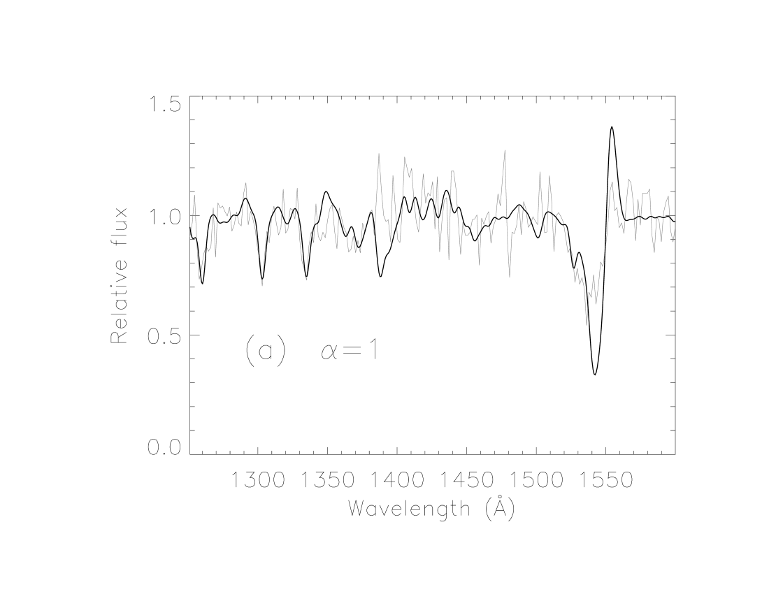
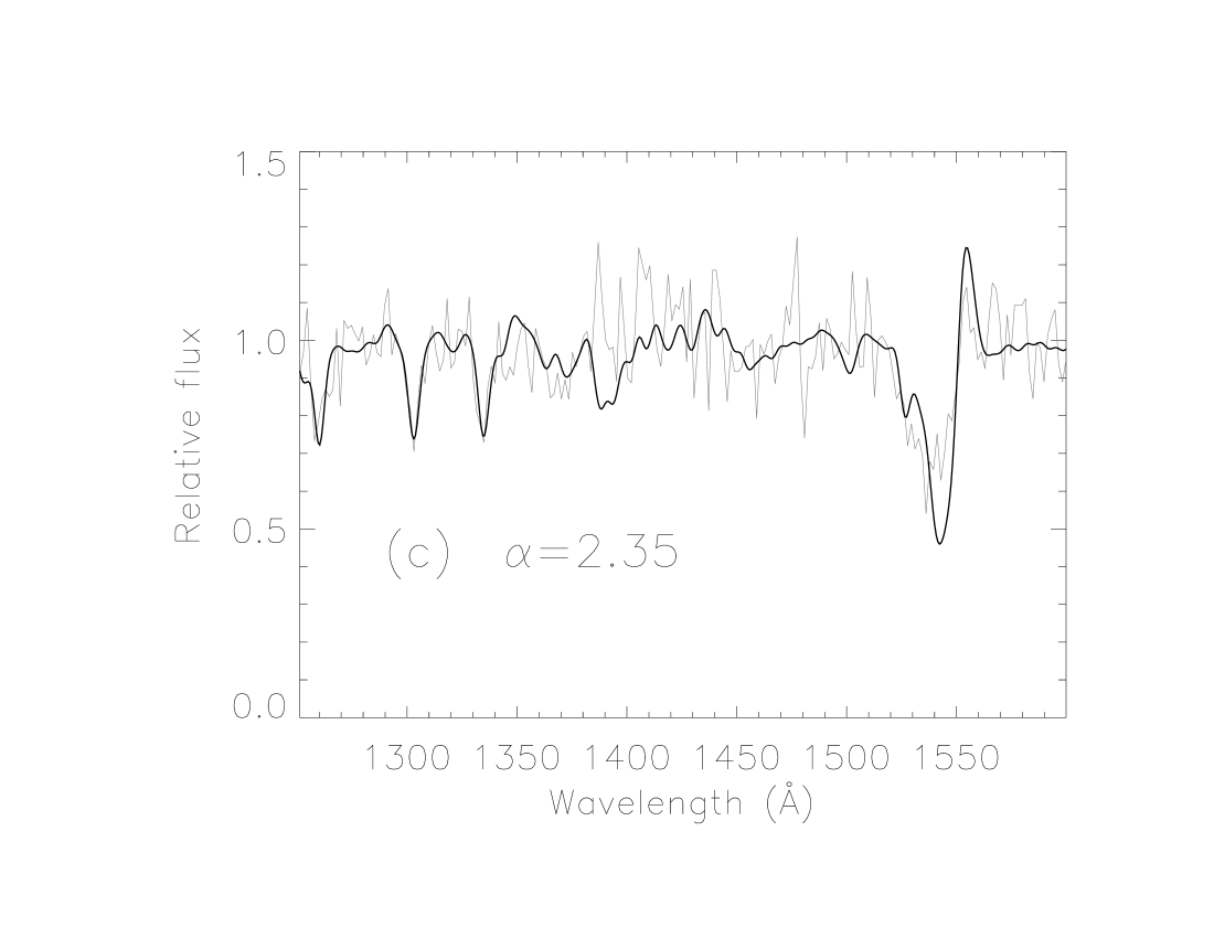
Figure 6: Observed vs. synthetic UV spectra for different IMF slopes. The synthetic spectra were convolved by a 5 Å FWHM Gaussian curve to match IUE’s resolution.

So far, we were unable to determine the IMF slope more accurately than constraining it to the range 1.5–3. Now, we show how we can discard IMFs flatter than $\alpha\approx 2$. Fig. 6 shows the observed and model UV spectra in the case of the IMF slopes $\alpha=1$, 1.7, 2.35 and 3, and for the best-fit metallicity (Z=0.008), age (2.8 Myr) and upper mass limit (120 M_☉). The synthetic UV spectra were created with the LMC/SMC library of Starburst99 (Leitherer et al. 2001). The depths of the SiIV $\lambda$1400 and CIV $\lambda$1550 lines were found to decrease with increasing IMF slope, due to the conservation of their equivalent widths and increase of their spectral widths. This result is in agreement with Robert et al. (1993). Due to excessive depths of the lines, the cases $\alpha=1$ and 1.7 were rejected, while we considered the fits reasonably good for the other, steeper IMF slopes.

5 Need to account for statistical fluctuations

In the previous section, we obtained a model attempting to reproduce as well as possible $W({\rm H}\beta)$, the numbers of WN stars and the UV stellar lines in the framework of a classical cluster analysis, that only takes into account the accuracy of the observational data. According to this model, the mass of the cluster is $\approx$3000 M_☉. Meanwhile, assuming a metallicity Z=0.004 and using the same evolutionary tracks, Mas-Hesse & Kunth (1999) obtained a cluster age $\tau=2.8$, an IMF slope $\alpha=1$ and a total mass of 534 M_☉, by the analysis of, mainly, the IUE-SWP and IUE-LWR spectra, but in absence of knowledge about the WR content of the cluster.

In both works, the results have been obtained under the following assumptions: correct stellar evolutionary tracks, instantaneous burst hypothesis and the implicit existence of a zero age main sequence (but see Tenorio-Tagle et al. 2003) and a number of stars in the cluster large enough to perfectly sample the IMF. However the estimated masses in both cases are about two orders of magnitude below the 10⁵ M_☉ mass for which, according to Cerviño & Mas-Hesse (1994), the whole IMF would be well filled. Hence, it is expected that sampling effects in the IMF will strongly affect any classical integrated analysis of this cluster.

Furthermore, the F439W luminosity of the cluster, with a value of -10.08 mag. is lower than the luminosity of the brightest star in the isochrone of the fitted model, -11.42 mag., that Cerviño & Luridiana (2004) showed to be the lowest luminosity limit under which a cluster cannot be modeled with classical population synthesis. Even worse, this limit is brighter than the entire cluster by as much as 1.4 magnitude. This implies that the results of classical synthesis models regarding magnitudes and colors can be strongly biased (Cerviño & Valls-Gabaud 2003). Unfortunately, the actual theoretical status of statistical modeling of stellar clusters is not ready yet to solve such a situation. The only realistic assessments that can be robustly obtained are: (i) due to the presence of at least one WN star, the age range is between 2.8 and 4.5 Myr (assuming there is no issue in isochrone computations and that WR star formation is not due to the evolution of binary systems), and (ii) the amount of gas transformed into stars at the onset of the burst does not exceed about 10⁴ M_☉ (for a Salpeter IMF and $m_{\rm low}=1$ M_☉), for which the luminosity of the cluster would reach the lowest luminosity limit.

This implies that the discussion about ages, IMF and discrepancies between the models and the observations in the analysis made with standard synthesis models hardly makes sense in our case.

One of our main objectives is to infer a plausible shape of the ionizing continuum, which implies the use of a technique different from the standard modeling as we show in the next section.

6 Star-by-star characterization of the cluster

Due to the small number of stars influencing the observables and the ionizing flux of the NGC 588 cluster, and because of the unsatisfactory results of the analysis detailed in Section 4, we decided to study not only the cluster as a whole, but also its individual stars. We achieved photometry of these stars, used isochrone curves to parameterize the cluster, attributed a model to each star, and synthesized spectra to be compared to the observations.

6.1 Stellar photometry

We performed photometric measurements of the stars on the five HST images, using the noao.digiphot.daophot package of IRAF. In each band, we ran daofind and phot to detect candidate stars and measure their intensities in 6 pixel radius apertures. The brightest isolated stars served to compute analytical PSFs for all the bands. We then ran allstar to reject the artifacts of the daofind routine and measure more accurately the intensities of the remaining objects. We selected again bright and isolated stars to carefully calculate the aperture corrections for the bands with the mkapfile routine of the noao.digiphot.photcal package, and derive the stellar intensities integrated over the full PSF extents. The intensities were corrected for charge-transfer inefficiency and filter contamination (see § 2.4), and converted into apparent magnitudes with the DN-to-flux keyword PHOTFLAM of the image headers,. The apparent magnitudes were converted into absolute (but reddened) magnitudes with the distance modulus 24.52 (Lee et al. 2002). The densest part of the cluster was not resolved by daofind, but from visual inspection, we found it to contain five clearly distinct stars. Using the Levenberg-Marquardt’s least-square method, and already knowing the PSF mathematical models, we fitted the positions and fluxes of these five stars in each of the images; we detected no other star in the residuals of the fits, and retained our five-star detection. The final photometric lists were composed of 536 stars in band F547M, 698 in F439W, 353 in F336W, 574 in F170W and 179 in F469N. 173 of them were common to bands F547M and F439W, 56, to F547M, F439W, F336W and F170W, and 20 to all bands. Table 4 lists the 56 stars common to F547M, F439W, F336W and F170W. In terms of absolute magnitudes, the 3$\sigma$ detection limits were estimated to be approximately $0.8$, $-0.1$, $-0.8$, $-3.8$ and $-2.8$ in filters F547M, F439W, F336W, F170W and F469N, respectively.

Star #	R.A.	Dec.	$M_{547}$	$M_{439}$	$M_{336}$	$M_{170}$	$M_{469}$	$E_{B-V}$	$m_{\rm ini}$
	01h32m	+30$\degr$							(M☉)
1	45.23s	38′58.4′′	$-6.63\pm$0.04	$-7.42\pm$0.03	$-8.14\pm$0.04	$-9.34\pm$0.04	$-7.26\pm$0.06	$0.11\pm$0.03${}^{\leavevmode\nobreak\ }$	55.3
2	45.56s	38′54.4′′	$-6.03\pm$0.04	$-6.91\pm$0.04	$-7.74\pm$0.03	$-9.32\pm$0.04	$-6.68\pm$0.08	$0.00\pm$0.03${}^{\leavevmode\nobreak\ }$	55.5
3	45.50s	39′07.0′′	$-6.12\pm$0.04	$-6.91\pm$0.03	$-7.55\pm$0.04	$-8.57\pm$0.05	$-7.09\pm$0.06	$0.11\pm$0.02${}^{\leavevmode\nobreak\ }$	43.8
4	45.31s	39′05.7′′	$-5.60\pm$0.05	$-6.45\pm$0.04	$-7.08\pm$0.04	$-8.24\pm$0.07	$-6.19\pm$0.09	$0.11\pm$0.03${}^{\leavevmode\nobreak\ }$	40.1
5	46.81s	39′06.9′′	$-5.34\pm$0.07	$-6.22\pm$0.05	$-6.89\pm$0.06	$-8.26\pm$0.08	$-5.91\pm$0.14	$0.08\pm$0.04${}^{\leavevmode\nobreak\ }$	38.1
6	45.37s	38′53.4′′	$-5.34\pm$0.07	$-6.19\pm$0.07	$-6.89\pm$0.06	$-8.33\pm$0.06	$-5.57\pm$0.13	$0.08\pm$0.04${}^{\leavevmode\nobreak\ }$	37.1
7	45.58s	38′55.5′′	$-4.86\pm$0.05	$-5.90\pm$0.05	$-6.55\pm$0.05	$-8.29\pm$0.06	$-5.02\pm$0.08	$0.02\pm$0.04${}^{\leavevmode\nobreak\ }$	32.1
8	45.37s	39′06.4′′	$-4.80\pm$0.07	$-5.59\pm$0.06	$-6.45\pm$0.06	$-7.73\pm$0.10	$-5.36\pm$0.15	$0.11\pm$0.02a	33.1
9	45.53s	38′54.9′′	$-4.64\pm$0.07	$-5.49\pm$0.06	$-6.35\pm$0.05	$-7.96\pm$0.07	$-5.04\pm$0.15	$0.07\pm$0.01a	32.1
10	45.60s	38′55.6′′	$-4.56\pm$0.06	$-5.31\pm$0.06	$-6.17\pm$0.06	$-7.46\pm$0.09	$-4.40\pm$0.08	$0.12\pm$0.01a	30.1
11	45.59s	38′55.4′′	$-4.27\pm$0.07	$-5.26\pm$0.06	$-5.78\pm$0.09	$-7.46\pm$0.09	$-4.85\pm$0.09	$0.09\pm$0.01a	29.1
12	45.47s	38′55.7′′	$-4.42\pm$0.06	$-5.19\pm$0.05	$-6.02\pm$0.06	$-7.51\pm$0.08	$-4.94\pm$0.15	$0.10\pm$0.01a	29.1
13	45.55s	38′55.3′′	$-4.28\pm$0.07	$-5.03\pm$0.07	$-5.93\pm$0.07	$-7.39\pm$0.09	$-4.77\pm$0.17	$0.10\pm$0.01a	27.1
14	45.59s	38′55.7′′	$-4.02\pm$0.09	$-4.90\pm$0.07	$-5.39\pm$0.09	$-6.93\pm$0.13	$-4.79\pm$0.09	$0.12\pm$0.02a	26.1
15	46.07s	39′02.5′′	$-4.10\pm$0.06	$-4.79\pm$0.06	$-5.51\pm$0.07	$-6.54\pm$0.14		$0.18\pm$0.02${}^{\leavevmode\nobreak\ }$	27.1
16	45.60s	38′55.4′′	$-3.87\pm$0.08	$-4.75\pm$0.07	$-5.37\pm$0.08	$-6.93\pm$0.11	$-4.45\pm$0.09	$0.10\pm$0.02a	24.4
17	45.80s	39′02.0′′	$-3.71\pm$0.07	$-4.50\pm$0.07	$-5.32\pm$0.07	$-6.63\pm$0.13	$-3.87\pm$0.27	$0.11\pm$0.02a	21.9
18	44.61s	38′52.6′′	$-3.35\pm$0.11	$-4.28\pm$0.08	$-4.88\pm$0.09	$-6.50\pm$0.12	$-3.04\pm$0.50	$0.08\pm$0.02a	20.1
19	45.42s	39′08.5′′	$-3.36\pm$0.08	$-4.22\pm$0.08	$-5.00\pm$0.08	$-6.16\pm$0.17	$-3.33\pm$0.42	$0.12\pm$0.02a	19.7
20	45.05s	38′55.2′′	$-3.28\pm$0.08	$-4.19\pm$0.07	$-5.01\pm$0.09	$-6.66\pm$0.11	$-3.60\pm$0.36	$0.05\pm$0.02a	19.5
21	45.54s	38′55.9′′	$-3.31\pm$0.11	$-4.14\pm$0.08	$-4.86\pm$0.10	$-6.44\pm$0.14		$0.08\pm$0.02a	19.1
22	45.20s	38′59.3′′	$-3.19\pm$0.13	$-4.07\pm$0.10	$-4.72\pm$0.14	$-6.08\pm$0.19		$0.11\pm$0.03a	18.6
23	45.10s	38′58.9′′	$-3.05\pm$0.08	$-3.99\pm$0.08	$-4.71\pm$0.10	$-6.13\pm$0.13	$-3.50\pm$0.35	$0.08\pm$0.02a	18.1
24	45.67s	38′57.4′′	$-3.09\pm$0.09	$-3.97\pm$0.09	$-4.55\pm$0.12	$-6.08\pm$0.14		$0.09\pm$0.02a	17.9
25	45.16s	39′04.2′′	$-3.05\pm$0.11	$-3.87\pm$0.11	$-4.15\pm$0.15	$-5.41\pm$0.20		$0.18\pm$0.03a	17.2
26	45.24s	38′56.2′′	$-2.94\pm$0.09	$-3.81\pm$0.09	$-4.37\pm$0.12	$-5.94\pm$0.15		$0.09\pm$0.02a	16.9
27	45.36s	38′54.6′′	$-2.86\pm$0.09	$-3.76\pm$0.08	$-4.42\pm$0.11	$-5.87\pm$0.16		$0.09\pm$0.03a	16.6
28	45.21s	38′55.8′′	$-2.85\pm$0.11	$-3.72\pm$0.09	$-4.28\pm$0.14	$-5.65\pm$0.21		$0.12\pm$0.03a	16.3
29	46.08s	39′01.7′′	$-2.93\pm$0.10	$-3.71\pm$0.10	$-4.03\pm$0.13	$-4.71\pm$0.32		$0.25\pm$0.04${}^{\leavevmode\nobreak\ }$	20.0
30	45.20s	38′54.2′′	$-3.07\pm$0.18	$-3.62\pm$0.10	$-4.12\pm$0.14	$-5.74\pm$0.19		$0.13\pm$0.04a	15.6
31	45.62s	38′58.6′′	$-2.75\pm$0.10	$-3.57\pm$0.09	$-4.47\pm$0.11	$-5.91\pm$0.20		$0.06\pm$0.03a	15.5
32	45.46s	38′54.5′′	$-2.64\pm$0.10	$-3.51\pm$0.09	$-4.26\pm$0.12	$-5.69\pm$0.19		$0.08\pm$0.03a	15.1
33	45.85s	39′07.1′′	$-2.52\pm$0.11	$-3.34\pm$0.10	$-4.07\pm$0.12	$-5.36\pm$0.24		$0.10\pm$0.04a	14.2
34	45.33s	38′56.7′′	$-2.39\pm$0.10	$-3.33\pm$0.10	$-4.10\pm$0.12	$-5.73\pm$0.17		$0.03\pm$0.03a	14.3
35	45.80s	39′11.5′′	$-2.34\pm$0.11	$-3.30\pm$0.09	$-4.01\pm$0.13	$-5.67\pm$0.19		$0.03\pm$0.03a	14.1
36	45.72s	39′10.6′′	$-2.33\pm$0.13	$-3.27\pm$0.11	$-3.89\pm$0.13	$-5.34\pm$0.23		$0.08\pm$0.04a	13.9
37	45.51s	38′55.9′′	$-2.42\pm$0.10	$-3.22\pm$0.09	$-3.70\pm$0.14	$-5.26\pm$0.24		$0.10\pm$0.04a	13.6
38	46.15s	38′56.7′′	$-2.32\pm$0.10	$-3.14\pm$0.11	$-3.74\pm$0.13	$-4.85\pm$0.28		$0.14\pm$0.04a	13.2
39	45.22s	38′54.7′′	$-2.39\pm$0.16	$-3.09\pm$0.14	$-3.77\pm$0.16	$-4.89\pm$0.29		$0.14\pm$0.05a	12.9
40	45.12s	38′55.8′′	$-2.40\pm$0.13	$-3.04\pm$0.12	$-3.84\pm$0.15	$-5.12\pm$0.24		$0.11\pm$0.04a	12.7
41	45.62s	38′54.2′′	$-2.27\pm$0.11	$-3.00\pm$0.11	$-3.69\pm$0.13	$-5.07\pm$0.25		$0.10\pm$0.04a	12.6
42	45.62s	38′57.8′′	$-2.06\pm$0.13	$-2.99\pm$0.12	$-3.67\pm$0.17	$-5.17\pm$0.25		$0.05\pm$0.04a	12.6
43	45.61s	38′55.1′′	$-2.39\pm$0.19	$-2.97\pm$0.17	$-3.60\pm$0.19	$-5.06\pm$0.30		$0.11\pm$0.05a	12.4
44	45.33s	38′55.8′′	$-2.16\pm$0.13	$-2.95\pm$0.12	$-3.70\pm$0.13	$-5.37\pm$0.26		$0.03\pm$0.04a	12.4
45	44.74s	38′55.8′′	$-1.78\pm$0.15	$-2.94\pm$0.13	$-3.07\pm$0.20	$-5.11\pm$0.29		$0.01\pm$0.05a	12.4
46	45.33s	38′53.0′′	$-2.23\pm$0.12	$-2.91\pm$0.12	$-3.66\pm$0.16	$-4.92\pm$0.28		$0.11\pm$0.05a	12.1
47	45.27s	38′58.6′′	$-1.98\pm$0.14	$-2.89\pm$0.13	$-3.56\pm$0.17	$-5.11\pm$0.25		$0.04\pm$0.04a	12.1
48	45.58s	38′55.8′′	$-2.32\pm$0.20	$-2.88\pm$0.19	$-3.94\pm$0.13	$-5.25\pm$0.26		$0.07\pm$0.05a	12.1
49	45.01s	38′50.9′′	$-1.90\pm$0.15	$-2.84\pm$0.12	$-3.54\pm$0.18	$-5.34\pm$0.28		$0.00\pm$0.05a	12.0
50	45.39s	38′55.6′′	$-1.91\pm$0.15	$-2.83\pm$0.14	$-3.50\pm$0.16	$-4.92\pm$0.30		$0.05\pm$0.05a	11.8
51	45.23s	38′54.9′′	$-2.04\pm$0.14	$-2.78\pm$0.15	$-3.37\pm$0.15	$-4.34\pm$0.44		$0.16\pm$0.07a	11.5
52	45.18s	38′53.0′′	$-1.81\pm$0.15	$-2.70\pm$0.13	$-3.26\pm$0.16	$-5.06\pm$0.26		$0.01\pm$0.05a	11.4
53	44.86s	38′57.5′′	$-1.60\pm$0.17	$-2.59\pm$0.14	$-3.01\pm$0.23	$-4.79\pm$0.31		$0.01\pm$0.06a	10.9
54	45.67s	38′54.7′′	$-1.67\pm$0.15	$-2.49\pm$0.17	$-3.18\pm$0.19	$-4.77\pm$0.29		$0.02\pm$0.05a	10.5
55	45.66s	38′53.2′′	$-1.36\pm$0.18	$-2.27\pm$0.17	$-2.94\pm$0.19	$-4.48\pm$0.42		$0.00\pm$0.07a	9.6
56	44.96s	38′55.7′′	$-1.30\pm$0.19	$-2.09\pm$0.19	$-2.84\pm$0.20	$-4.43\pm$0.48		$0.00\pm$0.08a	9.0

Table 4: Positions, reddened absolute magnitudes, $E_{B-V}$ coefficients, and initial masses of the brightest stars of NGC 588. The extinction is discussed in § 6.3.2, and the initial masses, in § 6.4. ^aValues eventually set to 0.11

The star observed with STIS is star #1 from Table 4. From the stars with available $M_{469}$, star #2 is the only one exhibiting a clear HeII excess, and was identified as the only or main WN star responsible for the HeII bump in the optical spectrum.

6.2 Identification of the star observed with STIS

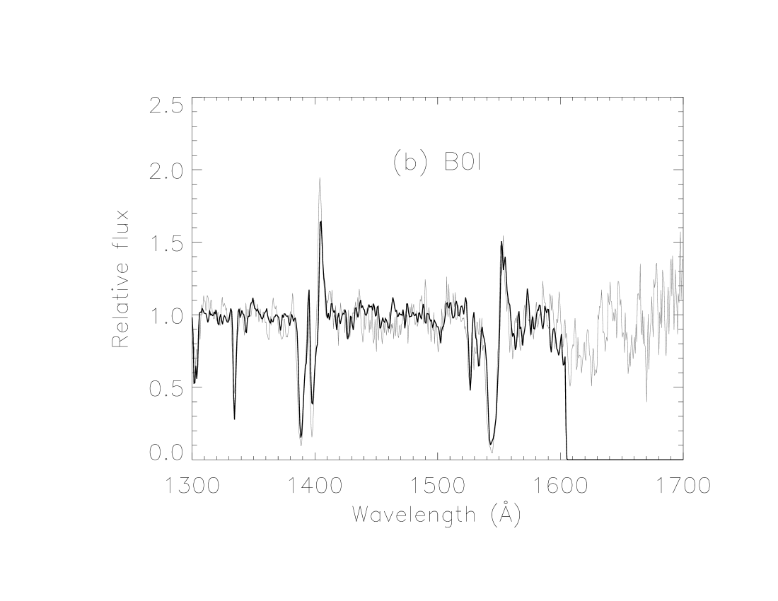
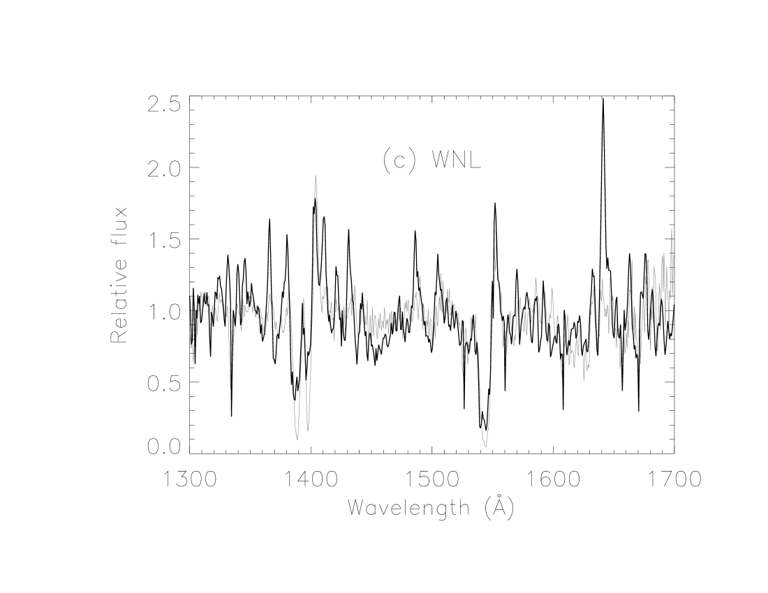
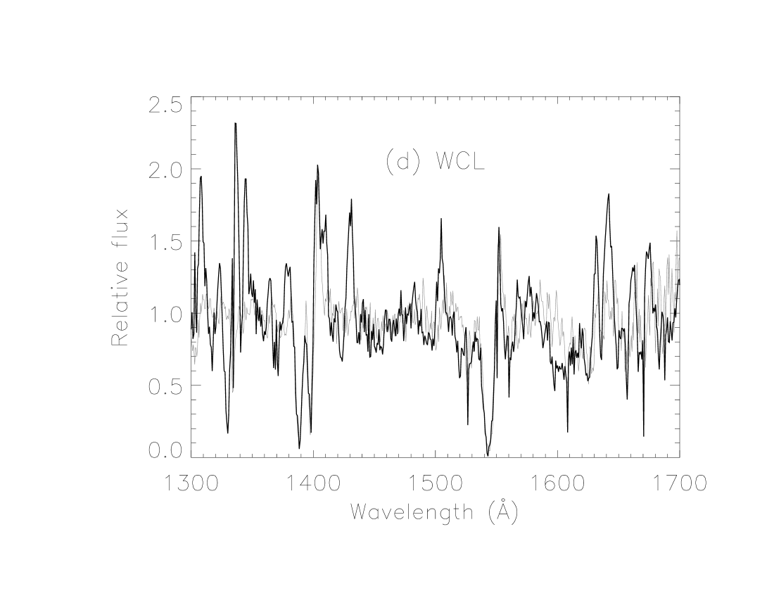
Figure 7: STIS vs. LMC/SMC spectra: B0II, B0I, WNL and WCL, respectively. The 1600–1700 Å region was unavailable for the B0I star.

Figure 8: Optical spectra near the WR HeII $\lambda$4686 bump, extracted from the blue CAHA spectrum around stars #1 and #2 of Table 4.

To identify the nature of the star observed with STIS, we first compared its spectrum with the ones of the LMC/SMC library of Leitherer et al. (2001), paying attention to the SiIV $\lambda$1400, CIV $\lambda$1550 and, when available, HeII $\lambda$1640 lines. The four acceptable matches (Fig. 7) indicated the star to be of class B0II, B0I, late WN (WNL) or late WC (WCL). We found a significant HeII $\lambda$4686 bump in the CAHA slit zone situated within the PSF extent of this quite isolated star (see Fig. 8 for this star and for star #2 of Table 4). The intensity of this bump being compatible with the (quite inaccurate) value derived from the photometric measurements, we deduced that the star is a WR. In absence of any optical carbon feature, in contrast with the well-defined HeII $\lambda$4686 bump, we concluded that it is a WNL star.

Considering the presence of such a star in the cluster, we inferred the age range of the latter for both metallicities Z=0.004 and Z=0.008: 3.2–3.7 and 2.8–4.5 Myr, respectively.

6.3 Comparison with isochrones

6.3.1 Construction of the isochrones

We constructed isochrone curves calling the same evolutionary tracks and model atmospheres as in Section 4. The effective temperatures and bolometric luminosities of these isochrones were computed with the original Starburst99 code. The corresponding magnitudes, however, were derived from them by means of an interpolation method different from the one of Starburst99. The latter mainly consists in nearest-neighbor selection of the spectra in the $(\log T_{\rm eff},\log g)$ plane, $T_{\rm eff}$ being the effective temperature, and $g$, the surface gravity. This induces step-like discontinuities in plots such as color-magnitude diagrams. This is why we exploited an alternative interpolation method, explicated in the Appendix, that consists, at each wavelength, of applying a bilinear interpolation of the logarithm of the flux in the $(\log g,y)$ plane, $y$ being a variable that depends both on the effective temperature and on the wavelength.

Depending on the stellar parameters, various kinds of model atmospheres, listed in Section 4, were exploited. This implies an artificial jump in the isochrone diagrams at the locus of transition from Lejeune et al. (1997) models to the one of Smith et al. (2002). Fortunately, this transition occurs in a zone where it is smaller than the error bars, and consequently it has a negligible impact.

6.3.2 Reddening

Figure 9: Illustration of the dereddening procedure. The isochrone shown here was established for an age of 3.5 Myr and for Z=0.008. Panel (a): observed $(M_{439},M_{336}-M_{547})$ diagram. Other panels: $(M_{439},M_{170}-M_{547})$ diagram dereddened with the $(M_{439},M_{336}-M_{547})$ one and the Galactic (b), LMC (c) and SMC (d) laws. The dotted lines are the WR branches of the isochrone curves. The two WR stars are signalized by open circles. The arrows indicate the shift that the observational points undergo by if dereddened for $E_{B-V}=0.1$. In the diagrams of panels (b), (c) and (d), the error bars account for uncertainties of $E_{B-V}$.

Figure 10: Same as Fig. 9 for the isochrone of 4.5 Myr.

Figure 11: Histogram of the dispersion of the stellar color excesses $E_{B-V}$ around the nebular one 0.11. The abscissa axis variable is the discrepancy term $\chi=(E_{B-V}-0.11)/\sigma(E_{B-V})$, where $\sigma(E_{B-V})$ is the uncertainty of the considered measurement of $E_{B-V}$. The histogram includes the 173 stars observed simultaneously through filters F547W and F439W. The overplotted curve is the theoretical expected distribution in the case of a unique real value $E_{B-V}=0.11$ and of well-determined measurement uncertainties.

We first investigated the extinction law, since a priori it may be different from the one inferred from the canonical study of the cluster (cf. § 4.1). We considered several isochrones in the age range of the cluster, and for each of them and each of the three tested extinction laws (Galactic, LMC and SMC), we proceeded as follows. We first estimated the color excess of each star in Table 4 by shifting the measured points towards the isochrone curve in the $(M_{439},M_{336}-M_{547})$ diagram according to the tested law, assuming stars #1 and #2 to be WN stars, and all the other ones to be on the main sequence. Then, we dereddened each star in the $(M_{439},M_{170}-M_{547})$ diagram, and compared the resulting points with the theoretical isochrone. Independently of the reference isochrone (i.e., in practice, the age), the SMC law was favored, as the systematic discrepancy between the isochrone and the locus of the stars, in particular the brightest ones, was small for the SMC law and significantly larger for the other two laws. Numerically, the discrepancy between the observational points in the $(M_{439},M_{170}-M_{547})$ diagram dereddened with the use of the $(M_{439},M_{336}-M_{547})$ one and the theoretical isochrone is characterized by a reduced $\chi^{2}$ ranging in the approximate intervals 2.3–3.3 for the Galactic law, 1.8–2.0 for the LMC one and 0.6–0.8 for the SMC one, obtained with 56 stars. The fact that this $\chi^{2}$ is close to 1 with the SMC law made us confident in the latter, and is also an indication that none of the 56 considered stars is significantly affected by blending with an unresolved companion. The procedure of selection of an extinction law is illustrated in Fig. 9 for an age of 3.5 Myr, and in Fig. 10 for 4.5 Myr.

Once the extinction law chosen, we re-considered the individual color excess $E_{B-V}$ of the stars. For the stars used in the selection of the extinction law, we started from the values already estimated in the $(M_{439},M_{336}-M_{547})$ diagram. For the stars that, once dereddened, were found to be brighter than $M_{439}=-6$, we conserved the values of $E_{B-V}$ found in this diagram and the corresponding uncertainties, the latter including the (small) scatters of values found with the different possible isochrones. However, for the stars dimmer than $M_{439}=-6$, we used the constancy of the isochrones in the $(M_{439},M_{170}-M_{547})$ diagram to estimate $E_{B-V}$ with better accuracy. Indeed, the uncertainty in $E_{B-V}$ determined in one of the $(M_{439},M_{X}-M_{547})$ diagrams ($X=170$ or $X=336$) is roughly the ratio $\sigma(M_{X}-M_{547})/(f_{X}-f_{547})$, where $\sigma(M_{X}-M_{547})$ is the uncertainty in the $M_{X}-M_{547}$ color, and in our case, this ratio in $E_{B-V}$ is smaller for $X=170$ than for $X=336$. With a few exceptions, we found all the color excess to be compatible with the nebular value, $E_{B-V}=0.11$, and when this was the case and the dereddened F439W magnitude was dimmer than $-6$, we set them to this value. An important departure from $E_{B-V}=0.11$ is the case of star #2: $E_{B-V}=0.00\pm 0.03$. All stars with unavailable F170W and F336W magnitudes were dereddened with $E_{B-V}=0.11$, compatible with the $(M_{439},M_{439}-M_{547})$ theoretical curve. Fig. 11 testifies to the correctness of setting almost all the 173 stellar color excesses to the nebular one.

In all what follows, the color-magnitude diagrams (CMDs) refer to the dereddened stellar magnitudes.

6.3.3 Fit of the age and of the metallicity

Figure 12: Observed vs. isochrone $(M_{439},M_{170}-M_{547})$ diagram for Z=0.004. The two WR stars are marked with open circles. The WR branches of the isochrones are shown as dashed lines.

Figure 13: Same as Fig. 12 for Z=0.008.

Figure 14: Final adopted $(M_{439},M_{170}-M_{547})$ diagram.

Figure 15: Final adopted HR diagram for all the detected stars. The circles show the selected individual stellar model. The dashed part of the diagram is the WR branch. The two dotted curves represent the HR diagram at 3.0 Myr (upper curve) and 5.5 Myr (lower curve)

The age and metallicity of the cluster were constrained by simultaneously fitting the isochrone to the dereddened observational points in the $(M_{439},M_{170}-M_{547})$ diagram, and by comparing synthetic spectra and derived properties to the observations. For a given isochrone, each star was identified to the nearest point of the isochrone in terms of chi-square (i.e., accounting for the error bars) in the $(M_{439},M_{170}-M_{547})$ diagram or, when the F170W magnitude was unavailable, in the $(M_{439},M_{439}-M_{547})$ diagram, thus attributing the most appropriate model spectrum to the considered star. If the cluster spectrum was synthesized to simulate what is seen through a slit (CAHA or IUE), the spectrum selected for a given star was multiplied by its corresponding aperture throughput (known from its position with respect to the slit and from the angular PSF or seeing of the considered data) and a function representing its possible differential extinction (with respect to the reference value $E_{B-V}=0.11$) along the processed wavelength range, and added to the total cluster spectrum to compute. If the total cluster spectrum was to be synthesized, then the individual stellar spectra were summed without being previously modified.

We computed the isochrone curves for the different ages multiple of 0.1 Myr belonging to the ranges constrained by the presence of a WNL star. Here, we show the curves obtained for the ages 3.2 and 3.7 Myr in the case Z=0.004 (Fig. 12), and 3.0, 3.5, 4.0 and 4.5 Myr for Z=0.008 (Fig. 13). At both metallicities, the isochrone high-luminosity main-sequence branch was found to move, with increasing age, from regions of low values of the $M_{170}-M_{547}$ color towards the somewhat “red” observational points.

The synthesized spectra were exploited as follows. For a given tested isochrone, the spectrum simulated for the optical slit was used to extract the model ratio $R_{B}=F_{\lambda}(3630)/F_{\lambda}(3780)$ related to the Balmer jump, which is a diagnostic of the effective temperature of a cluster dominated by hot stars. Indeed, in the spectrum of a hot star, the intensity of the Balmer jump decreases with increasing effective temperature, and usually serves to determine the subtypes of B stars, whereas it is negligible in the spectra of O stars. The observed value, whose uncertainty is dominated by the local fluctuating residues in photometric calibration, is $R_{B}=1.12\pm 0.08$. The constructed UV spectrum was visually compared to the IUE observed one. Finally, we derived the predicted $W({\rm H}\beta)$ from the total cluster spectrum, assuming again that the nebula absorbs all the ionizing photons, and thus requesting the predicted $W({\rm H}\beta)$ to be greater than or equal to the observed one.

Mathematically, we used the following $\chi^{2}$ estimator to constrain the age and the metallicity of the cluster:

$$\chi^{2} = \left(\frac{\max(330-W({\rm H}\beta),0)}{30}\right)^{2}+\left(\frac{R_{B}-1.12}{0.08}\right)^{2}$$

$$+\chi_{\rm isoc}^{2}$$ (2)

where $\chi_{\rm isoc}^{2}$ characterizes, for a given isochrone, the discrepancy between the latter and the loci of the brightest four MS stars in the $(M_{439},M_{170}-M_{547})$ diagram. The numerical results are summarized in Table 5. In practice, the synthetic Balmer jump was constant, and the fit was constrained by $W({\rm H}\beta)$ and $\chi_{\rm isoc}^{2}$. For Z=0.004, even at 3.7 Myr, the theoretical isochrone remained toward values of $M_{170}-M_{547}$ lower (“bluer”) than the observational points of the brightest stars, though the fit was acceptable. Meanwhile, for Z=0.008, the fit of the isochrone was very satisfactory for ages around 4.0 Myr, with $W({\rm H}\beta)$ also being well predicted. We retained the model with Z=0.008 and $\tau=4.2$ Myr as the best-fit one. The $(M_{439},M_{170}-M_{547})$ diagram for this model is shown in Fig. 14, and the corresponding Hertzsprung-Russel (HR) diagram, in Fig. 15. According to the classification of Schmidt-Kaler (1982), 20 stars were classified as O-type ones.

The SED of the best-fit model is shown in Fig. 16. We considered it to satisfactorily reproduce the observations, except for the strength of the optical WR bumps. However, the model atmospheres used for WR stars here are not intended to compute reliably these bumps, and we did not pay attention to their strength. Instead, we estimated them from Table 1 of Schaerer & Vacca (1998), knowing that star #2 was finally classified as a WNL from its hydrogen surface abundance. The results, satisfying but somewhat inaccurate (due in particular to the scatter of the model bump intensities), are summarized in Table 6. The synthetic UV spectrum, superimposed to the observed one in Fig. 17, was found to satisfactorily reproduce the CIV $\lambda$1550 line. It also contains an undetected SiIV $\lambda$1400 feature. However, the UV line spectrum is dominated by a small number of massive stars, that are not necessarily well represented by the spectra LMC/SMC library, in particular the WNL ones. In consequence, we did not consider the SiIV $\lambda$1400 discrepancy as a critical one.

	Z=0.004	Observed	Z=0.008
$\chi_{\rm isoc}^{2}$	5.2		2.3
$W({\rm H}\beta)$ (Å)	602	330$\pm$30	342
$R_{\rm B}$	1.10	1.12$\pm$0.08	1.10
age (Myr)	3.7 (3.7–3.7)		4.2 (3.6–4.4)

Table 5: Numerical results of the star-by-star analysis of the cluster. The parenthesized age ranges indicate the 90% confidence limits.

Quantity	$L$(HeII $\lambda$4686)	NIII $\lambda$4640/HeII $\lambda$4686
	(1035 erg s-1)
Observed	3.0$\pm$0.2	0.17$\pm$0.01
Model	13$\pm$9	0.2$\pm$0.1

Table 6: WR line strengths, observed/predicted in the dereddened CAHA spectrum.

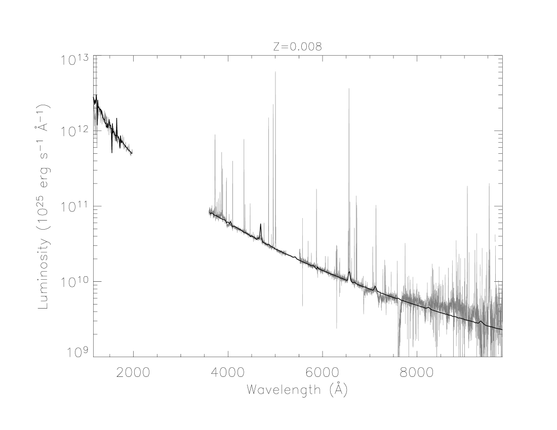
Figure 16: Optical and UV SEDs synthesized for Z=0.008 and $\tau=4.2$ Myr with the individual stellar models. For better visibility and comparison with Fig. 3, the luminosities of the observed optical and UV parts were rescaled with multiplicative factors, in order to fit the integrated luminosities in band F439W and F170W, respectively. The synthetic spectra were normalized using the same factors.

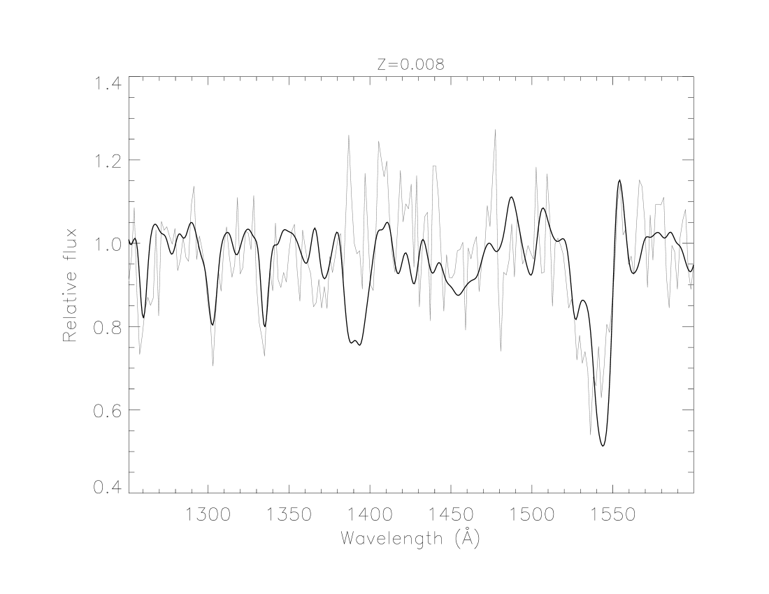
Figure 17: UV spectrum synthesized for Z=0.008 and $\tau=4.2$ Myr with the individual stellar models.

6.4 Mean IMF

Figure 18: IMF histogram and fit. Full line: best fit. Dashed line: fit for the Salpeter slope. The error bars are equivalent to 1$\sigma$ Gaussian ones, in terms of likelihood, and must be interpreted this way: for a model that goes through the extremity of an error bar, the observed value whose error bar is being considered has a likelihood to occur of $\exp(-1/2)$ times the maximum likelihood of the model at this abscissa.

From the initial mass associated with each star, we computed the mean power-law IMF of the cluster. More specifically, we constructed a histogram of the logarithm of the initial masses, from $\log(m)=0.8$ to $\log(m)=1.76$ ($m=6.3$ to $m=58$ M_☉), with a bin of 0.03 (equivalent to a factor of 1.07 between two successive bins), and fit it with an exponential law, assuming Poissonian noise in each bin, knowing that a power-law IMF $dN/dm\propto m^{-\alpha}$ can be translated into the law $dN/d\log(m)\propto 10^{(1-\alpha)\log(m)}$. The lower limit of the initial mass range was chosen in order to ensure that the stars of the cluster belonging to a given bin were all detected, and the upper limit corresponds to the highest possible initial mass at the age and metallicity of the cluster. The result is shown in Fig. 18. We found an IMF slope $\alpha=2.37\pm 0.16$, and retained the compatible Salpeter slope, resulting in an inferred IMF $dN/dm=(2680\pm 210)\,m^{-2.35}$. The corresponding total initial mass integrated in the range $1\leq m\leq 58$ M_☉ is $M_{\rm tot}=5800\pm 500$ M_☉.

7 Discussion

The most massive stars of an OB association are also the most influential ones, though the least numerous, on the spectrum of this cluster. In moderately massive clusters, their small number is subject to significant fluctuations around the mean IMF, causing large variations in the observable (near UV and optical) and Lyman continuum spectral ranges. For instance, in Section 4.5, we saw the significance of the presence of only 0.8 BSG in the analytical model of NGC 588 cluster upon the overall properties derived from this model. We now discuss the effects of the real sampling of the IMF in various mass ranges associated to different kinds of massive stars, and more generally in the mass range covered by the most luminous stars. Then, we present the results of a simulation of the effect of discrete random IMF sampling, in the whole initial mass range, over $W({\rm H}\beta)$.

7.1 Mean and observed numbers of different kinds of massive stars

From the mean IMF computed in Section 6.4, we derived the mean expected numbers of several kinds of massive stars susceptible to change significantly the spectral properties of the cluster. Here we present these results and discuss them.

7.1.1 Blue supergiants

According to our stellar models, at 4.2 Myr and for Z=0.008, BSGs (as defined in § 4.5) are stars with initial masses ranging from 44 to 55 M_☉. The number expectancy, derived from the integration, between these two limits, of the mean power-law IMF computed in § 6.4, is ${\mathcal{N}}({\rm BSG})=3.0$. The associated Poisson probability to observe no BSG, as is our case, is $\exp({\mathcal{N}}({\rm BSG}))=5$%. We added an artificial continuous population composed by this kind of stars, weighted by the Salpeter IMF slope, to the actual stellar content of the cluster. Independently of the optical absolute luminosity – which would be automatically fit in a classical modeling of the cluster – the most striking change in the computed spectral properties is, as expected, the large drop of $W({\rm H}\beta)$: in presence of the BSG population, the latter quantity would be only 133 Å, instead of 342 Å.

7.1.2 Wolf-Rayet stars

We computed the expected number of the different WR stars (WNL, WNE, WCL, WCE, WO), derived from the mean IMF of § 6.4; we found ${\mathcal{N}}({\rm WNL})=0.15$, ${\mathcal{N}}({\rm WNE})=0.02$, ${\mathcal{N}}({\rm WCL})=0.02$, ${\mathcal{N}}({\rm WCE})=0.01$ and ${\mathcal{N}}({\rm WO})=0.29$, according to the star classification of Starburst99. The resulting Poisson likelihood of the observed WR content of the cluster is 0.7%, a small value that is however much more satisfactory than the 0.04% likelihood derived from the analytical model. Furthermore, we simulated a spectrum obtained by replacing the two WR stars of the cluster with an analytical, complete population of 0.51 WN star following the Salpeter IMF. This population was expected to produce less luminous but possibly harder or softer radiation than the two actually detected WR, as the WR branch of the HR diagram (Fig. 15) spans a significant range of effective temperatures. We found that whereas $W({\rm H}\beta)$ is smaller with the modified stellar population, the latter produces harder radiation than the “true” one in the Lyman continuum range, especially below the threshold of ionization of He⁺, as summarized in Table 7.

BSG content	real	IMF	real	IMFa	2.8 Myra,b
WR content	real	real	IMF	IMFa	2.8 Myra,b
MS content	real	real	real	IMFa	2.8 Myra,b
$W({\rm H}\beta)$ (Å)	342	133	284	80	247
$Q({\rm H}^{0})$ ($10^{50}$ s-1)	2.14	2.16	1.39	0.54	1.60
$Q({\rm He}^{0})/Q({\rm H}^{0})$	0.13	0.12	0.14	0.11	0.14
$10^{8}$ $Q({\rm He}^{+})/Q({\rm H}^{0})$	9.3	8.0	2.8$\times$104	8.8	130
$Q({\rm O}^{+})/Q({\rm H}^{0})$	0.020	0.020	0.024	0.011	0.017

Table 7: Some spectral properties derived from the observed stellar content (2nd column) and from the one with BSG, WR and whole population replaced with the one predicted by the fitted power-law IMF (3rd, 4th and 5th columns, respectively). $Q(X)$ designates the photon rate able to ionize the ion “X” population of a nebula. ^aThe 5th and 6th columns correspond to analytical models, whose total mass here reproduce the observed F439W luminosity. ^bBest-fit model of the canonical analysis.

7.2 On the importance of the few most massive stars

In § 7.1.1 and 7.1.2, we saw the significance of fluctuations in the population of some characteristic kinds of massive stars upon the spectral properties of a cluster as moderately massive as the one of NGC 588. This issue can be generalized to all sorts of very massive stars, that can radiate intensely in the optical and/or ionizing spectral range and whose numbers are subject to the largest relative statistical fluctuations.

Figure 19: Top: SEDs of the whole cluster (full line), of the 6 brightest stars (dashed line) and of the remaining 167 stars (dotted line). Bottom: ratio of the brightest 6 stars SED (full line) and of the remaining 167 star SED (dotted line) to the total SED.

Figure 20: $(\log Q({\rm H}^{0}),M_{439})$ diagram of the detected stars along the the theoretical isochrone. The WR branch is the dashed part of the curve.

Figure 21: Star-by-star constructed SED (full lines), and SEDs of the analytical populations, for Z=0.008 and $m_{\rm up}=120$ M_☉, at 2.8 Myr (dashed line) and 4.2 Myr (dotted line).

In Fig. 19 are plotted the SEDs of the whole cluster, of the 6 brightest stars (in filter F439W) and of the remaining 167 stars, as well as the fractional contribution of the 6 brightest stars to the total SED. It is evident that these 6 stars are very influential on the total spectrum, whether at observable wavelengths (where they are responsible for about half the total flux) or in the high-energy range, where they generate approximately two thirds of the hydrogen-ionizing photons, even though they constitute only about 1/30 of the whole set of detected stars. These 6 stars, which also are the most massive ones, are specifically the stars situated in the temperature-luminosity zone that varies significantly within the first few millions of years of the cluster, as one can see in Fig. 15. Fig. 20 shows the $(M_{439},\log Q({\rm H}^{0}))$ diagram of the detected stars. The most striking feature is the quasi-vacuousness of the curve in the region of the 6 dominating stars, in particular the BSG branch that drops towards negligible Lyman continuum at high band F439W luminosities. If the IMF of the cluster were complete, as assumed in a classical model of stellar population, then the main spectral diagnostic, $W({\rm H}\beta)$, would be significantly lower than what we observe at the age and metallicity we derived from the star-by-star approach. This is illustrated in Fig. 21, where the SED found with the classical approach is also shown. In this figure, we can appraise the significance of the drop of the Lyman-to-optical continuum ratio, as well as the increase of the magnitude of the Balmer jump and the decrease of the global slope of the SED at observable wavelengths, when passing from the star-by-star SED to the one of the analytical model.

7.3 Approximate expected uncertainties and Monte-Carlo simulation

In Section 7.1 and 7.2, we saw the significant consequences of the deviation of the actual (discrete and statistically fluctuating) IMF of NGC 588 from the mean and continuously sampled analytical one. In this cluster of $\approx$6000 M_☉ (integrated in the interval of individual initial stellar masses 1–58 M_☉), the stars massive enough to rule its spectral properties, whether observable ($W({\rm H}\beta)$, Balmer jump, etc.) or not (e.g., hardness of the Lyman continuum), are only 6, which can easily explain the encountered issues.

Figure 22: Histogram of $\log W({\rm H}\beta)$ resulting from the 10⁶ Monte-Carlo discrete IMF realizations.

In order to estimate quantitatively the uncertainties related to the fluctuations of massive stellar populations of same age, metallicity and IMF as the ones of NGC 588, we performed a simple Monte-Carlo simulation where the mean IMF of § 6.4 was divided into 0.01 M_☉ wide mass bins, in which 1977 stars (1977 being the number of stars integrated in the mean IMF) were randomly distributed, according to the probability of each bin to be filled with a given star, this probability being given by the mean analytical IMF. We performed 10⁶ such Monte-Carlo realizations. This model assumes the stars of the cluster to have random masses, uncorrelated to each other (a simplification that may be corrected when the actual properties of star formation in clusters are better known), and following a likelihood function given by the mean IMF. For each random distribution, we calculated the resulting $W({\rm H}\beta)$; we found $\log(W({\rm H}\beta))$ to follow a roughly Gaussian distribution with standard deviation 0.24 dex (as also obtained analytically by Cerviño et al. 2002). The histogram of $\log(W({\rm H}\beta))$ is shown in Fig. 22. According to the simulation, the maximum-likelihood value of $W({\rm H}\beta)$ is 68 Å, and the 90% likelihood interval for this quantity is as wide as 40–244 Å. The observed value $W({\rm H}\beta)=330\pm 30$ Å is marginal, the likelihood of realizing a value greater than or equal to this one being $\approx$1%. This likelihood is of same order of magnitude as the 0.4% one to observe, as we do, no BSG and 2 WNL stars, given the mean IMF of the cluster.

Using the same kind of simulations, we established that, for the same IMF slope and cutoffs, the fluctuation of $W({\rm H}\beta)$ would still be $\approx$20% for a cluster as massive as $50\times 10^{3}$ M_☉.

8 Conclusions

In this work we have gathered the widest range of data available for the stellar cluster ionizing the giant HII region NGC 588, both imaging and spectroscopy, covering a wide wavelength range from the ultraviolet to the far red.

In the first part (Section 2 and 4), we showed the importance of endeavoring to obtain and process as numerous and accurate observable data as possible, in order to constrain models of the most common form of OB associations within the limits of the relevance of these models, rather than within the measurement errors and uncertainties. We discussed the problems encountered when fitting overall integrated nebular and stellar parameters, by means of a standard evolutionary population synthesis approach. In particular, by assuming an analytical IMF, the best fit model predicts the presence of BSGs simultaneous to the required (since observed) existence of WNs, and consequently predicts too a low value of $W({\rm H}\beta)$. This failure can be imputed mainly to two physical issues: the still important uncertainties in our knowledge of the evolution of massive stars (as reviewed by Massey 2003), and the effects associated with IMF sampling (as studied by Cerviño et al. 2002). We explored the latter in Section 5 through 7. In Section 6, we achieved quite a robust model of the cluster, and obtained good results. However, in this approach, we inferred a cluster age 50% higher than with the analytical approach, and a mass twice as large. In Section 7, we estimated the effects of departure of the observed set of stars from the one derived from the full sampling of the mean cluster IMF. In particular, we established that a diagnostic such as $W({\rm H}\beta)$ is very sensitive to the BSG content of the cluster, and that the hardness of the ionizing radiation, an unobservable spectral property that plays an important role in photoionization models of nebulae, depends significantly on the WR content. More generally, we assessed that the radiation field of NGC 588 is one among a large variety of possible SEDs for such a cluster, and that this is easily explained by the following statements: the most massive stars dominate the flux of the cluster both in the observable and Lyman-continuum wavelength ranges, show a wide variety of spectral properties, and are subject to strong population fluctuations.

We suggest three practical considerations that will help to better understand and characterize the evolutionary stage of massive ionizing star clusters: (i) A “best fit model” statement may not be very meaningful per se, and should not make us complacent that it implies the best solution. (ii) When possible, use color-magnitude diagrams to obtain the integrated properties of the ionizing cluster, as opposed to assuming a perfectly sampled mass function. (iii) Assess the importance of the few most massive stars on the overall SED of the cluster, both at ionizing and at non-ionizing wavelengths; this can be easily done by applying the lowest luminosity limit criteria established by Cerviño et al. (2003) and Cerviño & Luridiana (2004). If possible, use Monte-Carlo population models, provided they are relevant, and pending a more mature development of this approach to population synthesis.

We also established that the initial mass distribution of the stars detected in NGC 588 is compatible with a Salpeter IMF, if it is treated as a stochastic process.

Finally, in this work, we used the very common hypothesis of instantaneous starburst. However, recent works, like the one of Tenorio-Tagle et al. (2003), show that star formation in massive clusters spans time ranges such that the instantaneous formation hypothesis may not be valid for them. This statement does not call into question the significance of the disturbances caused by fluctuations in the high mass end of the IMF, but it is an additional uncertainty that is worth accounting for in further models of massive star clusters.

Appendix A Magnitude interpolation

At given age and metallicity, the isochrone data available from our programs consist in an array of physical parameters of model stars, each line containing the following parameters for the current star: the initial mass $M$, the effective temperature $T_{\rm eff}$, the bolometric luminosity $L_{\rm bol}$, and the surface abundances, in particular the hydrogen one $X$. From these parameters, we wanted to derive absolute magnitudes, to be compared to the observations, from atmosphere models. In our case, four kinds of models were available: Lejeune et al. (1997), Pauldrach et al. (2001), Hillier & Miller (1998) and black body. For each of the first three kinds of models, whose selection for given physical parameters was operated the same way as Starburst99 does, stellar fluxes are tabulated for a fix array of wavelengths and for various effective temperatures; in the case of Lejeune and Pauldrach models, the surface gravity $g$ is also present. When one of these grids is selected, Starburst99 performs nearest research interpolation along the $\log T_{\rm eff}$ axis (for Hillier grids) or in the $(\log T_{\rm eff},\log g)$ plane (for Lejeune and Pauldrach grids) to select a flux array, and normalizes the latter for its total to be equal to $L_{\rm bol}$. This non-continuous interpolation method can be exploited to compute the total spectrum of a model cluster, as the interpolation errors will tend to cancel each other. However, the resulting isochrone curve in a magnitude-magnitude of color-magnitude diagram will be irregular, with jumps resulting from the sudden transition from an array of the exploited grid to another. Here we suggest another form of interpolation to obtain more accurately determined model magnitudes.

Let us first consider the case of the black-body emission law: the wavelength-and-temperature-dependent flux is

$${\mathcal{B}}_{\lambda}(\lambda,T)=\frac{2\pi hc}{\lambda^{5}}\frac{1}{e^{hc/\lambda kT}-1}$$ (3)

The change of variable $x=hc/\lambda kT=1.44\times 10^{8}/\lambda T$ then gives:

$$\ln{\mathcal{B}}_{\lambda}(\lambda,T) = \ln\left(\frac{2\pi hc}{\lambda^{5}}\right)-\ln(e^{x}-1)$$ (4)

$$= \ln\left(\frac{2\pi hc}{\lambda^{5}}\right)-(x+\ln(1-e^{-x}))$$ (5)

This means that at a given wavelength $\lambda$, $\ln{\mathcal{B}}_{\lambda}(\lambda,T)$ is a linear function of the temperature-dependent variable $y=\ln(e^{x}-1)=x+\ln(1-e^{-x})$. This is the main idea underlying the interpolation of magnitudes from the grids of model stellar spectra. Indeed, the wavelengths covered by the HST filters F547M, F439W, F336W and F170W are line-free and keep quite far from the continuum jumps (in particular, the Balmer jump); hence at these wavelengths, we expect the stellar fluxes to behave nearly as in the black-body case. Consequently, we may calculate the flux predicted at wavelength $\lambda$, for the effective temperature $T_{\rm eff}$ and the gravity $g$, with the fluxes available in the grid in use at the two temperatures $T_{1}$ and $T_{2}$ that “surround” $T_{\rm eff}$, and at the same logarithmic surface gravity $L=\log g$, using the following linear interpolation formula:

$$\ln F_{\lambda}(\lambda;T_{\rm eff},L)\leavevmode\nobreak\ =\hskip 118.0pt$$

$$\frac{(y_{2}-y)\ln F_{\lambda}(\lambda;T_{1},L)+(y-y_{1})\ln F_{\lambda}(\lambda;T_{2},L)}{y_{2}-y_{1}}$$ (6)

This formula was straightly applied to the grids of Hillier model spectra, ignoring the $L$ variable which is undefined for these grids. For Lejeune and Pauldrach grids, we also needed to interpolate the fluxes as functions of $L$. This was done the following way:

• when, for the considered temperature, $T_{1}$ or $T_{2}$, at least two values of the surface gravity were available, the two ones closest to $g$, namely $g_{1}$ and $g_{2}$, were used to perform linear interpolation as a function of $L$:

  $$\ln F_{\lambda}(\lambda;T_{i},L)\leavevmode\nobreak\ =\hskip 131.0pt$$ (7)

  $$\frac{(L_{2}-L)\ln F_{\lambda}(\lambda;T_{i},L_{1})+(L-L_{1})\ln F_{\lambda}(\lambda;T_{i},L_{1})}{L_{2}-L_{1}}$$

• when only one value surface gravity was available in the grid (a marginal case that could occur with the Lejeune grids for the highest temperatures), its corresponding array of fluxes was adopted “as is”, i.e. neglecting the dependence of the stellar flux on gravity.

When using Lejeune or Pauldrach grids, the interpolation algorithm was finally the following:

1. in the grid, search for the two effective temperatures $T_{1}$ and $T_{2}$ nearest the temperature of interest $T_{\rm eff}$;

2. for each of both $T_{i}$, determine the two values $g_{i1}$ and $g_{i2}$ of the surface gravity closest to $g$, and calculate the array of fluxes $F_{\lambda}(\lambda;T_{i},\log g)$ by linear interpolation in the “segment” $[\log g_{i1},\log g_{i2}]$. If actually only one value of the gravity $g_{i}$ is available, then set $F_{\lambda}(\lambda;T_{i},\log g)=F_{\lambda}(\lambda;T_{i},\log g_{i})$;

3. at each wavelength, calculate $y$, $y_{1}$ and $y_{2}$, and apply formula (6) to determine the interpolated flux. Note that due to the fact that the variable $x=1.44\times 10^{8}/\lambda T$ could have values up to $\approx 800$, we used the formula $y=x+\ln(1-e^{-x})$ and not $y=\ln(e^{x}-1)$, as the latter would have caused floating overflows when running our codes ($e^{800}\sim 10^{347}$).

As we saw above, our interpolation method is meaningful for wavelength ranges where the stellar fluxes behave nearly as black-body ones. However, it does not apply at wavelengths of lines or near discontinuities (e.g., Lyman and Balmer jumps). The interpolation proposed here is preferred to calculate smoother running isochrone magnitudes, but does not involve a clear advantage to compute model spectra of clusters.