Weak Lensing Detection of Cl 1604+4304 at $z=0.90$

Abstract

We present a weak lensing analysis of the high-redshift cluster Cl 1604+4304. At $z=0.90$, this is the highest-redshift cluster yet detected with weak lensing. It is also one of a sample of high-redshift, optically-selected clusters whose X-ray temperatures are lower than expected based on their velocity dispersions. Both the gas temperature and galaxy velocity dispersion are proxies for its mass, which can be determined more directly by a lensing analysis. Modeling the cluster as a singular isothermal sphere, we find that the mass contained within projected radius $R$ is $3.69\pm 1.47\times({R\over 500{\rm kpc}})10^{14}$ $M_{\odot}$. This corresponds to an inferred velocity dispersion of $1004\pm 199$ km s^-1, which agrees well with the measured velocity dispersion of $989^{+98}_{-76}$ km s^-1 (Gal & Lubin, 2004). These numbers are higher than the $575^{+110}_{-85}$ km s^-1 inferred from Cl 1604+4304 X-ray temperature, however all three velocity dispersion estimates are consistent within $\sim 1.9\sigma$.

1 Introduction

Clusters of galaxies have historically been detected through their baryon content, either in optical/near-infrared surveys searching for overdensities of galaxies or in X-ray surveys searching for emission from the hot, intracluster medium. Previous observations have found strong differences between X-ray and optically-selected clusters at moderate-to-high redshift, implying that at least some massive clusters do not obey the local X-ray–optical relations. Specifically, the properties of the galaxies and the intracluster gas in local Abell clusters are strongly related. There exist well-defined correlations between the X-ray properties of the gas, such as luminosity ($L_{x})$ and temperature ($T_{x}$), and the optical properties of the galaxies, such as blue luminosity ($L_{B}$) and velocity dispersion ($\sigma$). These relations indicate that the galaxies and gas are in thermal equilibrium, i.e. $T_{x}\propto\sigma^{2}$ (Edge & Stewart 1991). Moderate-redshift clusters up to $z\sim 0.5$ exhibit the same X-ray–optical relations (Mushotzky & Scharf 1997; Horner 2001).

However, X-ray observations of all optically-selected clusters at $z\gtrsim 0.5$ indicate that they are weak X-ray sources, regardless of their measured richness or velocity dispersion, with luminosities of only a few $\times 10^{44}$ ergs s^-1 (Castander et al. 1994; Bower et al. 1997; Holden et al. 1997; Donahue et al. 2001; Lubin, Oke, & Postman 2002; Lubin, Mulchaey & Postman 2004). Consequently, many optically-selected clusters do not obey the local $L_{x}-\sigma$ relation. Their X-ray luminosities are low for their velocity dispersions, indicating that optically-selected clusters at these redshifts are underluminous (by a factor of $3-40$) compared to their X-ray–selected counterparts. These results seem to imply that, at least for some clusters, the galaxies and gas are no longer in thermal equilibrium and that the clusters are still dynamically young. Strong observational evidence, such as double peaks, significant substructure, and/or a filamentary appearance in the gas, galaxy, and total mass distributions, does indicate that many (if not most) clusters at these redshifts are actively forming (see e.g., Lubin & Postman 1996; Henry et al. 1997; Gioia et al. 1999; Della Ceca et al. 2000; Ebeling et al. 2000; Jeltema et al. 2001; Stanford et al. 2001; Hashimoto et al. 2002; Maughan et al. 2003; Huo et al. 2004)

Cl 1604+4304 at $z=0.90$, orginally detected in the Gunn, Hoessel & Oke (1986) survey, is typical of optically-selected clusters at these redshifts. Velocity dispersions measured first by Postman et al. (2001) and more accurately by Gal & Lubin (2004) indicate that the system is massive, equivalent to an Abell richness class 1–2 cluster. It has, however, only a modest X-ray luminosity and temperature of $L_{x}=2.0\times 10^{44}$ h${}_{70}^{-2}$ ergs s^-1 and $T_{x}=2.51^{+1.05}_{-0.69}$ keV, respectively (Lubin et al. 2004). Based on its measured velocity dispersion of $989^{+98}_{-76}$ km s^-1, Cl 1604+4304 is cooler by a factor of 2–4 compared to the local $\sigma-T_{x}$ relation.

Gas temperature and galaxy velocity dispersion are only proxies for mass, which can be determined directly by a lensing analysis. The mass determined by lensing is independent of the cluster’s dynamical state, star formation history, and baryon content (Smail, Ellis & Fitchett 1994; Smail et al.  1995). As a result, we have undertaken a weak lensing analysis of Cl 1604+4304 using deep imaging from the Keck 10-m telescope. Because weak lensing uses the background galaxy population, it becomes progressively more difficult to apply to high-redshift clusters. The highest-redshift cluster previously detected with lensing is MS 1054-03, a very X-ray luminous, hot, massive cluster at $z=0.83$ (Luppino & Kaiser 1998; Hoekstra, Franx, & Kuijken 2000). Its X-ray luminosity is $1.6\times 10^{45}$ h${}_{70}^{-2}$ ergs s^-1, and estimates of its X-ray temperature range from 7.2${}^{+0.7}_{-0.6}$ keV to 12.3${}^{+3.1}_{-2.2}$ keV (Gioia et al.  2004 and references therein). Hoekstra et al.  (2000) determined MS 1054-03 weak lensing mass to be $(1.2\pm 0.2)\times 10^{15}$ within 1 Mpc radius, corresponding to a velocity dispersion of $1311^{+83}_{-89}$ km s^-1 for an isothermal sphere, in very good agreement with the spectroscopicaly measure of $1153\pm 80$ km s^-1 (Gioia et al.  2004; Tran et al.  in preparation).

Although Cl 1604+4304 has a substantially lower gas luminosity and temperature than MS 1054-03, it may be more typical of galaxy clusters at these redshifts because the number density of very X-ray luminous clusters declines significantly at redshifts of $z>0.6$ (e.g., Mullis et al. 2004).

In addition to deep imaging, weak lensing analyses of high-redshift clusters requires better knowledge of the source redshift distribution. To calibrate the mass of a lens, one must know the mean distance ratio of the sources. For typical source redshifts around unity, uncertainties of the order of 10% in the source redshift distribution matter little for a low-redshift cluster, but they represent a large systematic error when the lensing cluster is itself at a redshift of $z\sim 1$. Here, the tail of the source redshift distribution is behind the cluster, and it becomes crucial to minimize the errors in estimating this tail. In this paper, we introduce a new method of estimating the source redshift distribution based on degrading higher-quality data rather than estimating the faint tail of one’s own data. In §2 & 3, we describe the data and our weak lensing analysis. In §4, we summarize our results and discuss future plans for a more accurate weak lensing measurement of this cluster.

2 The Data

The imaging used in the weak lensing analysis was obtained on 27 July 1999 at the Keck 10-m telescope using the Low Resolution Imaging Spectrograph (LRIS; Oke et al. 1986). The pixel scale of LRIS is $0.215^{\prime\prime}$, and its field of view is approximately $5.0^{\prime}\times 6.5^{\prime}$. The seeing was excellent at $0.60^{\prime\prime}$ full-width-half-maximum (FWHM) in the center of the image, with some degradation to an average of $0.75^{\prime\prime}$ at the edges. Twenty-nine $R$-band images with exposure times of 300 sec each were taken. A dither pattern of $40^{\prime\prime}$ in width was used to minimize the effect of bad columns and bright stars. Conditions were not photometric; however, photometric calibration was obtained from a shallower observation of the same area, with the same instrument, on a photometric night. These calibration images were taken as part of the Oke et al. (1998) survey of nine high-redshift clusters of galaxies (see also Postman et al. 1998, 2001).

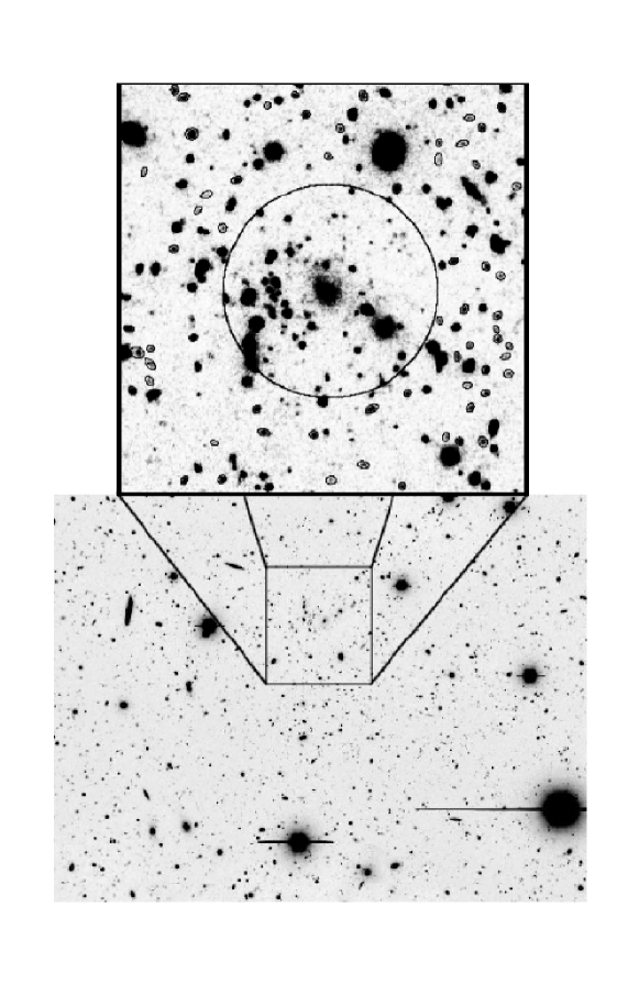
Figure 1: Deep R imaging. Left panel: entire $5.0^{\prime}\times 6.5^{\prime}$ field of view. Right panel: $1.5^{\prime}\times 1.5^{\prime}$ zoom around the cluster optical center. The circle indicates the inner cut in radius (objects too close to the center were excluded from the lensing analysis), and contours are shown for objects used in the weak lensing analysis (all with $R>25$).

The imaging data was reduced using standard IRAF routines, with the usual corrections (including bias and flatfielding) being applied. Individual exposures were aligned and co-added to create a single, deep $R$-band image with an effective exposure time of 8700 sec. The final image is shown in the left panel of Figure 1. To perform our weak lensing analysis, the intrinsic anisotropy of the point-spread function (PSF) has to be corrected. The left panel of Figure 2 shows the ellipticity and position angles of 127 stars as a function of position, before correction. The mean ellipticity is $9\%$, with a rms of $5\%$, and the position angles are highly spatially correlated. We convolved the image with a kernel with ellipticity components opposite to that of the PSF at each point (Fischer & Tyson, 1997). However, the 3$\times$3 pixel kernel used was not large enough to correct the PSF completely in one pass. Therefore we iterated four times, until improvement stopped. Each iteration also allowed us to clip a few more interloping compact galaxies from the PSF sample, leaving a clean sample of 127 stars at the end. The right panel of Figure 2 shows the result. The mean ellipticity decreased to $4\%$ with a $3\%$ rms, and the position angles are no longer spatially correlated. After rounding, the final FWHM varied from $0.65^{\prime\prime}$ at the center to an average of $0.85^{\prime\prime}$ at the edges.

The object detection and photometry was performed with SExtractor version 2.2.2 (Bertin & Arnouts, 1996), resulting in a catalog of 4424 objects (136 per arcmin²). The galaxy counts peak at $R\approx 27$, and the magntiude limit is $R=29$ for a 5$\sigma$ detection.

3 The Weak Lensing Analysis

We measure weighted moments of objects using the ellipto software described in (Bernstein & Jarvis, 2002), discarding any sources which triggered error flags. We also use their seeing correction procedure, which corrects for the dilution of the shear signal due to the isotropic smearing of the PSF. We discarded sources which were not at least 25% larger than the PSF at that position, rather than apply a large and noisy correction. Because of the strong stellar size dependence with position on the CCD (up to 30%), a second order spatial fit was used in the the seeing correction. This spatial variation in the size selection function does not bias the shapes of the objects, but it does impose a spatial variation on the source redshift distribution, which will be discussed below.

Objects with ellipticity greater than 0.6 tend to be blends of multiple sources and were also excluded from the lensing analysis. The number of objects passing all these quality checks is 1588 (49 per arcmin²).

We measure the tangential shear around the cluster optical center, using background galaxies with $R>25$ (see right panel of Figure 1). Because the area closest to the core is expected to be dominated by cluster members, we use only sources at Radius $>25^{\prime\prime}$ for the weak lensing analysis. The final number of galaxies is 1053.

Figure 3 shows the mean tangential shear for four annuli around the optical center, with 1$\sigma$ errors attached. As a null test, we also show in open circles the other (45^∘) shear component, which is consistent with zero as expected. These measurements are also indicated in Table 1. The tangential shear is detected at 1.8 and 2.0$\sigma$ respectively in the two inner points, which has only a 2.5% probablility of happening randomly. Hence the detection confidence is 97.5%. We do not expect to detect shear in the outer two points, given the redshift and velocity dispersion previously measured for this cluster (see below). As a measurement of the expected level of PSF systematics, we also show in Figure 3 that the “tangential shear” computed from the stars is consistent with zero.

To avoid the mass sheet degeneracy inherent in mass reconstructions of small fields, we fit a model to the shear profile. Given the low signal to noise, we choose to fit the simplest possible model, a singular isothermal sphere, to all four points. Assuming a cosmology of $H_{0}=70$, $\Omega_{m}=0.3$, and $\Omega_{\Lambda}=0.7$, we find that $\gamma_{t}=(0.054\pm 0.021)\times({R\over{500~{}{\rm kpc}}})^{-1}$. The $\chi^{2}$ for this fit is 1.25 for three degrees of freedom, hinting that the errors may have been overestimated. As a control, we fit an SIS to the 45-degree component of the shear and found 0.027 $\pm$ 0.022, with a $\chi^{2}$ of 4.09 for three degrees of freedom.

To determine the mass, we must know the cluster redshift and the source redshift distribution. For any given mass, the tangential shear is proportional to the combination of angular diameter distances from the observer to the lens ($D_{L}$), from the observer the source ($D_{S}$), and from the lens to the source ($D_{LS}$):

$$\gamma^{t}\propto{{D_{L}D_{LS}}\over{D_{S}}}$$

The cluster has a spectroscopic redshift of $z=0.9001$ (Gal & Lubin, 2004). The challenge then is to estimate $\langle{{D_{L}D_{LS}}\over{D_{S}}}\rangle$ for the source population. This is not the same as estimating the mean redshift of the sources, because the relation is quite nonlinear, and only sources with redshifts of $z>0.9$ have a non-zero contribution. For high-redshift lenses, the estimation of the higher-redshift tail can be little more than guesswork unless additional data are brought to bear.

We estimate the source redshift distribution by degrading the Hubble Deep Field North (HDF-N), which has a well-known redshift distribution, to match our data. This is a more stable approach than attempting to extrapolate the ditribution from our data alone, because many of the background galaxies are near the faint limit of our survey. First, we convolve the F606W (which is the closest match to our filter) HDF-N image (Williams et al. , 1996) with $0.65^{\prime\prime}$ and $0.85^{\prime\prime}$ FWHM gaussian to simulate the range of PSF sizes in the Keck image. Then, we re-pixelize, add noise, and catalog the image to match the Keck data. We judge the match to be satisfactory because the galaxy counts $N({\rm mag})$ in the degraded HDFN and Keck catalogs are very similar.

We then apply the same magnitude and size cuts used in the lensing analysis of the Keck image, and look up their photometric redshifts (Fernandez-Soto et al. , 1999). Figure 4 shows the mean photometric redshift and $1\sigma$ scatter as a function of magnitude for both PSF sizes. The histogram indicates the distribution of magnitudes of the lensing sources in Cl1604. Throughout the relevant magnitude range, the mean source redshift is nearly constant at $z=1.45$. We convert each source photometric redshift to a distance ratios ${{D_{L}D_{LS}}\over{D_{S}}}$, and take the mean. This mean, $386.8\pm 23.2$ Mpc, corresponds to an effective source redshift of $1.31\pm 0.04$. Again, this is not the same as the mean source redshift ($z=1.45$).

Finally, we check that the magnification provided by the cluster does not significantly change the source redshift distribution near the cluster center. Figure 5 shows the magnification for a source at $z=1.31$ expected for a 1004 km s^-1 cluster at $z=0.90$, as a function of projected radius. It is at most 0.4 mag, at the innermost radius used for tangential shear measurement. Because of the nearly constant redshift distribution seen in Figure 4, this additional depth has negligible impact on the effective source redshift.

The relative uncertainties of the shear and the distance ratio statistics are shown in Figure 6. The shaded areas indicate 1, 2 and 3$\sigma$ confidence limits for the fit shown in Figure 3. Combining the shear measurement with the mean distance ratio, the weak lensing mass estimate for this cluster is $3.69\pm 1.47\times({R\over 500~{}{\rm kpc}})10^{14}$ $M_{\odot}$. This corresponds to an inferred velocity dispersion of $1004\pm 199$ km s^-1, which agrees with the measured velocity dispersion of $989^{+98}_{-76}$ (Gal & Lubin, 2004). Our weak lensing measurement is also reasonably consistent with the velocity dispersion ($\sigma_{v}$) inferred from the X-ray temperature ($T_{x}$) of Cl 1604. Using the best-fit to the $\sigma_{v}-T_{x}$ relation for clusters at $z<0.5$ (Mushotzky & Scharf 1997; Horner 2001), the measured temperature of $2.51^{+1.05}_{-0.69}$ keV (Lubin et al. 2004) implies a velocity dispersion of $575^{+110}_{-85}$ km s^-1 which is consistent within $\sim 1.9\sigma$. However, given the large non-statistical scatter in the local $\sigma_{v}-T_{x}$ relation, the differences between the velocity dispersion measurements may be well less than 2$\sigma$.

4 Summary

We report the weak lensing detection of Cl 1604+4304 at a redshift of $z=0.90$. This is the highest-redshift cluster yet detected with weak lensing. We find a mass estimate of $3.69^{+1.47}_{-1.46}\times({R\over 500~{}{\rm kpc}})10^{14}$ $M_{\odot}$, independent of the cluster’s dynamical state. This mass estimate is in good agreement with the spectroscopic velocity dispersion.

Unfortunately, we cannot measure the optical mass-to-light ratio (M/L) because the small field does not provide adequate control regions. A wider field would serve three purposes: (1) provide control regions for the luminosity distribution, (2) allow a direct mass reconstruction without mass sheet degeneracy, and (3) show the larger scale structure associated with Cl 1604+4304. The former benefit is of great interest because we know that Cl 1604+4304 is a member of a supercluster which contains at least four massive clusters and extends up to $\sim 100$ Mpc (Gal & Lubin, 2004). Because the dynamics of such a large scale structure are very complex, mass measurements which do not rely on galaxy velocities are essential. In addition to a wide field, one must also go extremely deep in good seeing conditions to perform an adequate weak lensing analysis of clusters at $z\sim 1$. The combination of wide and deep, now available at a few facilities such as the Subaru telescope in conjunction with Suprime-Cam (Miyazaki et al. 2002), offers the possiblity of constraining the mass of $z\sim 1$ clusters, including Cl 1604+4304, independent of their star formation history or dynamical state.

Table 1: Shear as a function of radius

Radius (arc sec)	$\gamma_{t}$	$\sigma(\gamma_{t})$	$\gamma_{45^{\circ}}$	$\sigma(\gamma_{45^{\circ}})$
32	0.136	0.074	0.048	0.076
61	0.076	0.039	-0.025	0.042
110	0.009	0.025	0.037	0.025
193	0.012	0.028	0.047	0.029

Figure 2: Point-spread function correction. Shapes of stars, which as point sources should be perfectly round, are represented as sticks encoding ellipticity and position angle. Left panel: raw data with spatially varying PSF ellipticities up to 23% (mean of 9%). Right panel: after convolution with a spatially varying asymmetric kernel, ellipticities are vastly reduced (stars with $\epsilon<0.5\%$ are shown as dots), and the residuals are not spatially correlated as a lensing signal would be.

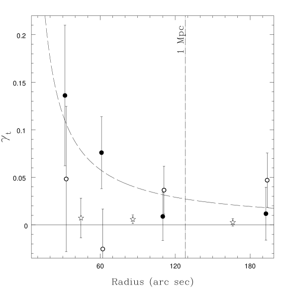
Figure 3: Tangential shear, centered on the cluster optical center (solid circles), as a function of radius, with 1$\sigma$ errors shown. The dashed curve shows the best-fit isothermal sphere. The open circles indicate the $45^{\circ}$ shear component, which should average to zero. The open stars indicate the level of PSF systematics computed from the stars (the radii are different because there are not enough stars to subdivide the stars in four annulii).

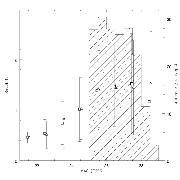
Figure 4: Mean redshift and $1\sigma$ scatter as a function of magnitude for HDFN simulations at $0.65^{\prime\prime}$ (squares) and $0.85^{\prime\prime}$ (triangles) seeing. Mean redshifts are computed discarding objects that would not be used in the lensing analysis. The histogram indicates the distribution of magnitudes of lensing sources in Cl1604.

Figure 5: Expected magnification of a source at $z=1.31$ by a 1004 km s^-1 cluster at $z=0.90$, as a function of projected radius. Also shown are the Einstein radius ($R_{E}$),and the inner ($R_{I}$) and outer ($R_{F}$) radii inside which the shear was computed.

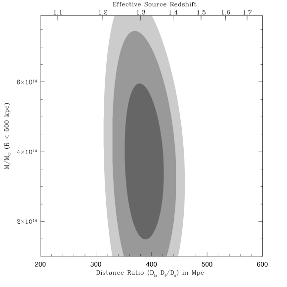
Figure 6: Shear and distance ratio relative uncertainties. The shaded areas indicate 1, 2 and 3$\sigma$ confidence limits for the fit shown in Figure 3. For reference, we also show the effective source redshift on the top.

References

- Bernstein & Jarvis (2002) Bernstein, G.M. & Jarvis, M. 2002, AJ, 123, 583.
- Bertin & Arnouts (1996) Bertin, E., & Arnouts, S. 1996, A&A, 117, 393.
- (3) Bower, R.G., Castander, F.J., Couch, W.J., Ellis, R.S., & Bohringer, H. 1997, MNRAS, 291, 353
- (4) Castander, F.J., Ellis, R.S., Frenk, C.S., Dressler, A., & Gunn, J.E. 1994, ApJ, 424, L79
- (5) Della Ceca, R., Scaramella, R., Gioia, I.M., Rosati, P., Fiore, F., & Squires, G. 2000, å, 353, 498
- (6) Donahue, M. et al. 2001, ApJ, 552, 93
- (7) Ebeling, H. et al. 2000, ApJ, 534, 133
- (8) Edge, A.C., & Stewart, G.C. 1991, MNRAS, 252, 428
- Fernandez-Soto et al. (1999) Fernandez-Soto, A., Lanzetta, K.M., Yahil, A., 1999, 513, 34.
- Fischer & Tyson (1997) Fischer, P., & Tyson, J.A. 1997, AJ, 114, 14.
- Gal & Lubin (2004) Gal, R.R., & Lubin, L.M. 2004, ApJ, 607, 1.
- (12) Gioia, I.M., Henry, J.P., Mullis, C.R., Ebeling, H., & Wolter, A. 1999, AJ, 117, 2608
- Gioia et al. (2004) Gioia, I.M., Braito, V., Branchesi, M., Della Ceca, R., Maccacaro, T., & Tran, K.-V. 2004, A&A, 419, 517
- (14) Gunn, J.E., Hoessel, J.G., & Oke, J.B. 1986, ApJ, 306, 30
- (15) Hashimoto, Y., Hasinger, G., Arnaud, M., Rosati, P., & Miyaji, T. 2002, å, 381, 841
- (16) Henry, J.P., Gioia, I.M., Mullis, C.R., Clowe, D.I., Luppino, G.A., Boehringer, H., Briel, U.G., Voges, W., & Huchra, J.P. 1997, AJ, 114, 1293
- Hoekstra, Franx, & Kuijken (2000) Hoekstra, H., Franx, M., & Kuijken, K. 2000, ApJ, 532, 88
- (18) Holden, B.P., Romer, A.K., Nichol, R.C., & Ulmer, M.P. 1997, AJ, 114, 1701
- (19) Horner, D. 2001, Ph.D. thesis, Univ. Maryland
- (20) Huo, Z., Xue, S., Xu, H., Squires, G., & Rosati, P. 2004, AJ, 127, 1263
- (21) Jeltema, T.E., Canizares, C.R., Bautz, M.W., & Malm, M.R. 2001. ApJ, 562, 124
- (22) Lubin, L.M., & Postman, M. 1996, AJ, 111, 1795
- (23) Lubin, L.M., Oke, J.B., & Postman, M. 2002, AJ, 124, 1905
- Lubin, Mulchaey, & Postman (2004) Lubin, L.M., Mulchaey, J.S., Postman, M. 2004, ApJ, 601, 9.
- Lubin et al. (2000) Lubin, L.M., Brunner, R., Metzger, M.R., Postman, M., & Oke, J.B. 2000, ApJ, 531, L5 J.E., Hoessel, J.G., Schneider, D.P. 1998, AJ, 116, 584
- Luppino & Kaiser (1997) Luppino, G.A. & Kaiser, N. 1997, ApJ, 475, 20
- (27) Maughan, B.J, Jones, L.R., Ebeling, H., Perlman, E., Rosati, P., Frye, C., & Mullis, C.R. 2003, ApJ, 587, 589
- Miyazaki et al. (2002) Miyazaki, S., et al. 2002, PASJ, 54, 833
- Mullis et al. (2004) Mullis, C.R., Henry, J.P., Forman, W., Gioia, I.M., Hornstrup, A., Jones, C., McNamara, B.R., & Quintana, H. 2004, ApJ, 607, 175
- (30) Mushotzky, R.F., & Scharf, 1997, ApJ, 482, 16
- Oke et al. (1995) Oke, J.B., Cohen, J.G., Carr, M., Cromer, J., Dingizian, A., Harris, F.H., Labrecque, S., Lucinio, R., Schaal, W., Epps, H., & Miller, J. 1995, PASP, 10, 375
- Oke et al. (1998) Oke, J.B., Postman, M., & Lubin, L.M. 1998, AJ, 116, 549
- Postman et al. (1998) Postman, M., Lubin, L.M., & Oke, J.B. 1998, AJ, 116, 560
- Postman et al. (2001) Postman, M., Lubin, L.M., & Oke, J.B. 2001, AJ, 122, 1125
- Smail et al. (1994) Smail, I., Ellis, R.S., Fitchett, M.J., 1994, MNRAS, 270, 245-270
- Smail et al. (1995) Smail, I., Ellis, R.S., Fitchett, M.J., Edge, A.C., 1995, MNRAS, 273, 277-294.
- (37) Stanford, S.A. et al. 2001, ApJ, 552, 504
- Williams et al. (1996) Williams, R. E., et al. 1996,AJ, 112, 1335.