Abstract

We present 86 GHz ($v=1,J=2\rightarrow 1$) SiO maser line observations with the IRAM 30-m telescope of a sample of 441 late-type stars in the Inner Galaxy ($-4\degr<l<+30\degr$). These stars were selected on basis of their infrared magnitudes and colours from the ISOGAL and MSX catalogues. SiO maser emission was detected in 271 sources, and their line-of-sight velocities indicate that the stars are located in the Inner Galaxy. These new detections double the number of line-of-sight velocities available from previous SiO and OH maser observations in the area covered by our survey and are, together with other samples of e.g. OH/IR stars, useful for kinematic studies of the central parts of the Galaxy.

Abstract

We present a compilation and study of DENIS, 2MASS, ISOGAL, MSX and IRAS 1–25$\mu$m photometry for a sample of 441 late-type stars in the inner Galaxy, which we previously searched for 86 GHz SiO maser emission (Chapter II). The comparison of the DENIS and 2MASS $J$ and K_S magnitudes shows that most of the SiO targets are indeed variable stars. The MSX colours and the IRAS $[12]-[25]$ colour of our SiO targets are consistent with those of Mira type stars with dust silicate feature at 9.7 $\mu$m feature in emission, indicating only a moderate mass-loss rate.

Abstract

We have computed extinction corrections for a sample of 441 late-type stars in the inner Galaxy using the 2MASS near-infrared photometry of the surrounding stars and assuming the intrinsic source colours. From this, the near-infrared power law is found to be A${}_{\lambda}\propto\lambda^{\mathrm{-}1.9\pm 0.1}$. Near- and mid-infrared colour-colour properties of known Mira stars are also reviewed. From the distribution of the dereddened infrared colours of the SiO target stars we infer mass-loss rates between $10^{-7}$ and $10^{-5}$ M_⊙ yr^-1.

Abstract

We present a study of DENIS, 2MASS, ISOGAL and MSX photometry for a sample of evolved late–type stars in the inner Galaxy, which we previously searched for 86 GHz SiO maser emission (Messineo et al. 2002). Bolometric magnitudes are computed for each SiO star by direct integration of the observed energy distribution, and bolometric corrections as a function of colours are derived. Adopting a distance of 8 kpc the SiO stars within 5 from the Galactic Centre show a distribution of bolometric magnitudes that peaks at $M_{\mathrm{bol}}=-5.1$ mag, i.e., very similar to the OH/IR stars close to the Galactic centre. From their bolometric luminosities and interstellar extinction we find that 11% of the SiO stars are likely to be foreground to the bulge. Furthermore the small velocity dispersions of those foreground stars suggest a disk component. The 15 known large amplitude variables included in our sample fall above the Mira period–luminosity relation of Glass et al. (1995), which suggests a steepening of the period–luminosity relation for periods larger than 450 days, as also seen in the Magellanic Clouds. From this period–luminosity relation and from their colours, the envelopes of SiO stars appear less evolved than those of OH/IR stars, which have thicker shells due to higher mass–loss rates.

Promotiecomissie  

Promotor :	Prof. dr. H. J. Habing
Referent :	Dr. J. Lub
Overige leden :	Prof. dr. W. B. Burton
	Dr. M.R. Cioni (European Southern Observatory, Garching bei München)
	Prof. dr. K. Kuijken
	Prof. dr. K. M. Menten (Max-Planck-Institut fuer Radioastronomie, Bonn)
	Prof. dr. A. Omont ( Institut d’Astrophysique de Paris)
	Prof. dr. P. T. de Zeeuw

A Lucia e Leonardo

Front cover: “I Girasoli” by Renato Guttuso. Permission to reproduce this painting was kindly granted by Dr. Fabio Carapezza Guttuso and authorised by SIAE 2004 (Italian Society of Authors and Publishers).
Back cover: ISOGAL image taken at 7 $\mu$m (LW5 filter) of a field of 20$\times$20centred on $(l,b)=-0.27^{\circ},-0.6^{\circ}$, field FC–00027–00006.  

Chapter 0 Introduction

The Milky Way is the cornerstone of our understanding of galaxies. The structure and kinematics of its gas and stars can be studied in unique detail due to their relative proximity. However, being located well within the Galactic disk and thereby observing the Milky Way in non–linear projection makes it difficult to properly map its large-scale morphology.

One of the interesting findings has been that observations of molecular line emission (CO, HI) and stellar motions show signatures of a Galactic Bar in the inner Galaxy. However, its characteristics such as elongation, thickness and viewing angle are still poorly constrained. One of the main obstacles has been the strong obscuration by interstellar dust toward the inner Galaxy, which makes optical studies of the stellar population in that region almost impossible. The extinction is less severe at near- and mid-infrared wavelengths. To characterise the structure and formation history of the Milky Way, several infrared surveys were conducted during the past decade: ISOGAL, MSX, DENIS, 2MASS. These data contain a wealth of information on the structure of the stellar populations that has yet to be fully analysed. Having entered a golden age for Galactic astronomy, soon even more detailed imaging and spectroscopy will be provided by the Spitzer Space Telescope, while the GAIA satellite will provide unprecedented astrometry.

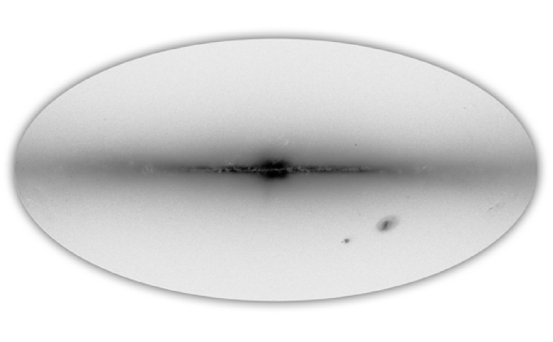
Figure 1: This infrared image taken by the 2MASS satellite shows the plane of our Milky Way Galaxy as a thin disk. Dust obscuration makes the optical appearance of the Milky Way much more patchy.

My thesis research has focused on the structure and stellar population of the inner 4 kpc of the Milky Way. I have analysed data from recent infrared surveys and obtained SiO radio maser line observations of late-type giants to study the star formation history and the gravitational potential of the inner Galaxy. With ages ranging from less than 1 to 15 Gyr, the infrared-luminous late-type giant stars are representative of the bulk of the Galactic stellar population, and hence trace its star formation history. Their spatial abundance variation maps the stellar mass distribution, and thereby probes the Galactic gravitational potential. The reddening of their spectral energy distribution can be used to map the interstellar extinction. Their envelopes often emit strong molecular masers (OH, SiO) that can be detected throughout the Galaxy, and through the precise measurement of the maser line velocity they reveal the stars’ line-of-sight velocities. Therefore they are ideal tracers of the Galactic kinematics and gravitational potential.

1 Late-type giants

In this section I shall briefly discuss the life cycle of stars, with emphasis on the red giant and asymptotic giant branch phases.

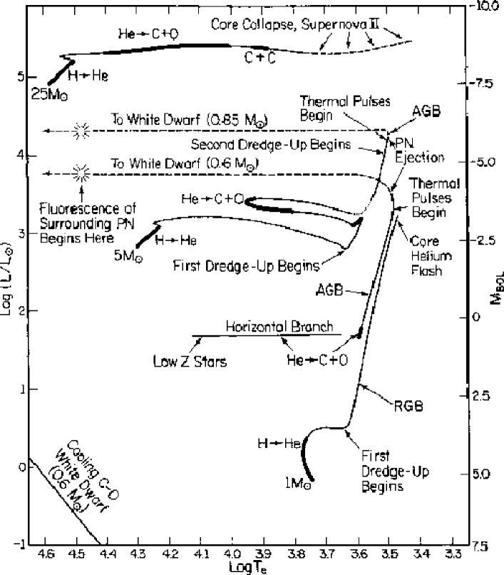
Figure 2: Stellar evolution tracks of 1, 5, and 25 M_⊙ stars in the H-R diagram (Iben 1985).

A low- to intermediate-mass star ($M_{*}<8\,M_{\odot}$) spends 80 to 90 percent of its life on the so called main-sequence phase. This phase ends when a large fraction of the star’s hydrogen has been converted to helium. Then the stellar core contracts and heats until hydrogen fusion starts in a shell surrounding the core. This causes the stellar envelope to expand to about 50 to 100 solar diameters, while the surface temperature decreases. Stars in this phase are called red giant branch (RGB) stars.

When the core temperature is high enough, helium nuclei fuse into carbon and oxygen. For stellar masses less than 2.3 solar masses (low mass stars), the core is degenerate and core helium burning begins abruptly in a so called core helium flash. In the Hertzsprung-Russell (HR) diagram this event marks the tip of the red giant branch. For higher mass stars helium burning begins more gradually. The core helium-burning phase lasts between 10 and 25 percent of a star’s main-sequence lifetime.

When the core helium is exhausted, the core contracts, the envelope expands and the stellar surface temperature decreases. The star is now powered by hydrogen and helium burning in shells surrounding the core, which consists of carbon and oxygen nuclei with a degenerate distribution of electrons. A star in this phase is called an asymptotic giant branch (AGB) star. This name originates from the fact that in the HR diagram for low mass stars the AGB branch approaches the RGB sequence asymptotically. They can be as large as several hundred solar radii and have a relatively cool surface temperature of about 3000 K.

At the beginning of the AGB phase, helium shell burning prevails over shell hydrogen burning, so the C-O core grows steadily in mass, approaching the hydrogen shell (E-AGB). When the mass of helium between the core and the hydrogen shell drops below a critical value, the helium shell exhibits oscillations that eventually develop into the first helium shell flash and the thermally pulsating (TP-AGB) phase begins. A dredge-up (the third dredge-up) may take place during this phase, bringing carbon to the surface.

Mass-loss reduces the envelope mass until the residual envelope is ejected in a short superwind phase. The strength of the wind controls the decrease of the stellar mass (as the star climbs the AGB in the HR diagram), which also affects the evolution of its surface composition. Mass-loss may occur also in RGB stars close to the RGB tip, but with much lower intensity than in AGB stars.

The third dredge-up is fundamental to explain the conversion of a fraction of oxygen-rich AGB stars into carbon-rich AGB stars (for which [C/O]$>1$) and predicts that the latter form only above a specific minimum luminosity. Carbon stars are virtually absent in the Galactic bulge, whereas they are numerous in the Magellanic Clouds, suggesting that the lower metallicity there provides for a more efficient dredge-up.

AGB stars produce roughly one third of the carbon in the Galaxy, almost the same amount as supernovae and Wolf-Rayet stars. By returning dust and gas to the interstellar medium, RGB and AGB stars pave the way for the formation of future generations of stars and planets.

Due to their low surface temperatures, late-type giants (RGB and AGB) are bright at infrared wavelengths. Facing a high interstellar extinction toward the central regions of the Milky Way that obscures stars at visible wavelengths, red giants are the best targets for studies of the stellar populations, dynamics, and star formation history in the inner Galaxy.

1 AGB star and variability

An important property of AGB stars with direct applications to Galactic structure studies is their luminosity variability. The radial pulsations of AGB stars are confined to the large convective envelopes and should not be confused with the thermal pulse that originates in the helium burning shell. The latter leads to a longer-term variability.

Variable AGB stars are named in several different ways based on the light curve properties and periods: large amplitude variables (LAV), long period variables (LPV), Mira variables, semiregular (SR) and irregular variables.

By definition, Mira stars show pulsations with large amplitudes at visual wavelengths (more than 2.5 mag) and vary relatively regularly with typical periods of 200 to 600 days. Semiregular variables show smaller amplitudes (less than 2.5 mag) and they have a definite periodicity. Since they are obscured in the visual, this classification cannot be applied to inner Galactic variable AGB stars. Therefore, for inner Galactic variable stars ‘LAVs’ and ‘LPVs’ refer to variations in the $K$-band. Mira stars are usually LAVs with $K$-band variation amplitudes larger than 0.3 mag.

Another important class of AGB variable stars are OH/IR stars, which are dust-enshrouded infrared variable stars. They are discovered in the infrared and show 1612 MHz OH maser emission. Their periods are typically longer than 600 days and can exceed 1500 days.

Recent observations from the MACHO, EROS and OGLE surveys initiated a discussion on the pulsation modes of long period variables and on the period-luminosity relations. Such period-luminosity relations are important for Galactic structure studies as they yield estimates for a star’s distance. The new data reveals four parallel period-luminosity sequences (A-D). However, the classical period-luminosity relation discovered by Feast et al. (1989), which is based on visual observations of Mira stars, still holds and coincides with the C sequence. Large amplitude variables with a single periodicity, like probably most of our SiO targets, populate this sequence.

2 Circumstellar maser emission

MASER stands for Microwave Amplification by Stimulated Emission of Radiation. In 1964 Charles Townes, Nicolay Gennadiyevich Basov and Aleksandr Mikhailovich Prochorov received the Nobel Prize for their discovery of the maser phenomenon. Now, forty years later, we know of thousands of astronomical masers, “radio radiation detected in some lines of certain astronomical molecules, attributed to the natural occurrence of the maser phenomenon” (Elitzur).

Maser radiation is caused by a population inversion in the energy levels of atoms or molecules. The non-equilibrium inversion is caused by different pumping mechanisms, in astronomical objects usually infrared radiation and collisions.

An observed line can be identified as a maser line on the basis of its unusually narrow line-width, or when line ratios indicate deviations from thermal equilibrium.

Various molecules can show maser emission. Astronomical masers are found around late-type stars (circumstellar masers), and in the cores of dense molecular clouds (interstellar masers). A comprehensive review of astronomical masers was given by Elitzur (1992) and Reid & Moran (1988). In this thesis we study circumstellar maser emission.

The circumstellar envelopes of oxygen-rich late-type stars can exhibit maser emission from SiO, H₂O, and OH molecules (Habing 1996). Masers occur in distinct regions at various distances from the central star. SiO masers at 43 and 86 GHz originate from near the stellar photosphere, within the dust formation zone (Reid & Menten 1997). Water masers originate further out, at distances of up to $10^{15}$ cm from the central star, while OH masers are found in the cooler outer regions of the stellar envelope, about ten times further out.

The presence or absence of particular maser lines in a circumstellar envelope appears to depend on the opacity at 9.7$\mu$m: a higher mass-loss rate leads to a more opaque dust shell, which shields molecules better against photodissociation by interstellar UV radiation.

SiO masers arise from rotational transitions in excited vibrational states. These levels can be highly populated only near the star where the excitation rates are high. SiO maser emission has been detected in different transitions towards oxygen-rich AGB stars (i.e. Mira variables, semi-regular variables, OH/IR stars) and supergiants. The relative intensity of different SiO maser lines varies among different sources, indicating that the SiO maser pumping mechanism depends on the mass-loss rate. Maser pumping is dominantly radiative, as suggested by the observed correlation between the maser intensity and the stellar infrared luminosity. However, collisional pumping cannot be ruled out. A maser line can show the stellar line of sight velocity with an accuracy of a few km s^-1.

H₂O (22 GHz) and OH (1612 MHz, 1667 MHz and 1665 MHz) masers originate from transitions in the ground vibrational state. H₂O maser spectra are irregular and variable. Therefore they are not useful for an accurate determination of stellar line of sight velocities. The 1612 MHz OH maser line is pumped by radiation from the circumstellar dust, which excites the 35 $\mu$m OH line and has a typical double-peaked profile. The stellar velocity lies between the two peaks and the distance between the two peaks yields a measure of the expansion velocity of the circumstellar envelope.

Lewis (1989) analysed colours of and masers from IRAS stars, suggesting a chronological sequence of increasing mass-loss rate: from SiO, via H₂O to OH masers. This sequence links AGB stars via the Mira and OH/IR stages with Planetary Nebulae. However, parameters other than mass-loss, such as stellar abundance, probably also play an important role (Habing 1996).

2 The Milky Way galaxy

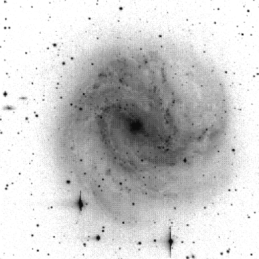
Figure 3: The Southern Pinwheel galaxy, M83, was classified as intermediate between normal and barred spiral galaxies by G. de Vaucouleurs. It has both a pronounced disk component exhibiting a spiral structure, and a prominent nuclear region, which is part of a notable bulge/halo component. The Milky Way might look similar to M83.

Our home Galaxy, the Milky Way, is a large disk galaxy. It is likely to be of Hubble type SBbc, with its main components being the bulge, the disk, and the halo.

The Milky Way today is the result of star formation, gas flow, and mergers integrated over time. The different Galactic components were not formed by independent events, and their formation history is largely unknown. The possible connection between the star formation history and the formation of Galactic structures is equally unknown.

Halo
The halo is composed of a dark matter and a stellar halo. The dark halo is of yet unknown nature and dominates the total Galactic mass, as suggested by dynamical studies of satellite galaxies. The stellar halo, a roughly spherical distribution of stars whose chemical composition, kinematics, and evolutionary history are quite different from stars in the disk, contains the most metal-poor and possibly some of the oldest stars in the Galaxy. It retains important information on the Galactic accretion history. The recent discovery of stellar streams in the halo (e.g. Helmi et al. 1999; Ibata et al. 1994) supports the hierarchical clustering and merging scenario of galaxy formation.

Disk
The disk is usually divided into two components, the thin and thick disks. The thick disk (Gilmore & Reid 1983) is older that 10 Gyr. Its metallicity ranges from -1.7 to -0.5 [Fe/H], it has a scale height of 0.7-1.5 kpc, a scale length of 2-3.5 kpc and a vertical velocity dispersion of 40 km s^-1. The thin disk has a scale-height of about 250 pc and contains stars of all ages. The thick disk was probably formed from the thin disk during a merger event that heated the disk (Gilmore et al. 2002).

Bulge
There is some confusion in the use of the term “bulge”. In the literature it is often used to indicate everything in the inner few kiloparsec of the Galaxy, i.e., the bar and the nuclear disk. Wyse et al. (1997) prefer to define a “bulge” as a “centrally concentrated stellar distribution with an amorphous, smooth appearance. This excludes gas, dust and recent star formation by definition, ascribing all such phenomena in the central parts of the Galaxy to the central disk, not to the bulge with which it cohabits.”

The “bulge” is dominated by an old stellar component (10 Gyr). Its abundance distribution is broad, with a mean of [Fe/H]$\sim-0.25$ dex (McWilliam & Rich 1994). It has a scale height of about 0.4 kpc, and a radial velocity dispersion of about 100 km s^-1.

There is growing evidence of a non-axisymmetric mass distribution in the inner Galaxy. This is found from the near-infrared light distribution, source counts, gas and stellar kinematics, and microlensing studies. However, it is not clear yet whether a distinction should be made between the triaxial Galactic bulge and the bar in the disk – a bar is defined as a thin, elongated structure in the plane.

In face-on galaxies, it is not unusual to observe both a central bulge and a bar (i.e. NGC1433). In general, bars may be populated by both old and young stars. In addition, barred galaxies often show a ring around the bar. From studies of edge-on galaxies there is indication that peanut-shaped or box-shaped (rather than spheroidal) bulges may be associated with bars. The Milky Way provides the closest example of a box-shaped bulge, and therefore it is a unique laboratory to investigate the structure and kinematics of a boxy bulge and its relation with the disk. A bar and a triaxial bulge could both be present, distinct, and coexisting.

The existence of a distinct disk-like dense molecular cloud complex in the central few hundred pc of our Galaxy, the Central Molecular Zone (CMZ), was established in the early 1970s. Observations of ongoing star formation and the presence of ionizing stars suggest that this is a component different from the bulge. In the longitude-velocity diagram (Fig. 4) it generates a remarkable feature called the 180 pc-Nuclear Ring. It can be understood as a gaseous shock region at the transition between the innermost non intersecting X1 orbits and the X2 orbits (Binney et al. 1991). The total mass of the CMZ (including the central stellar cluster) amounts to $(1.4\pm 0.6)10^{9}M_{\odot}$, of which 99% is stellar mass, and 1% gaseous mass. Its stellar luminosity amounts to $(2.5\pm 1)10^{9}L_{\odot}$, 5% of the total luminosity of the Galactic disk and bulge taken together (Launhardt et al. 2002).

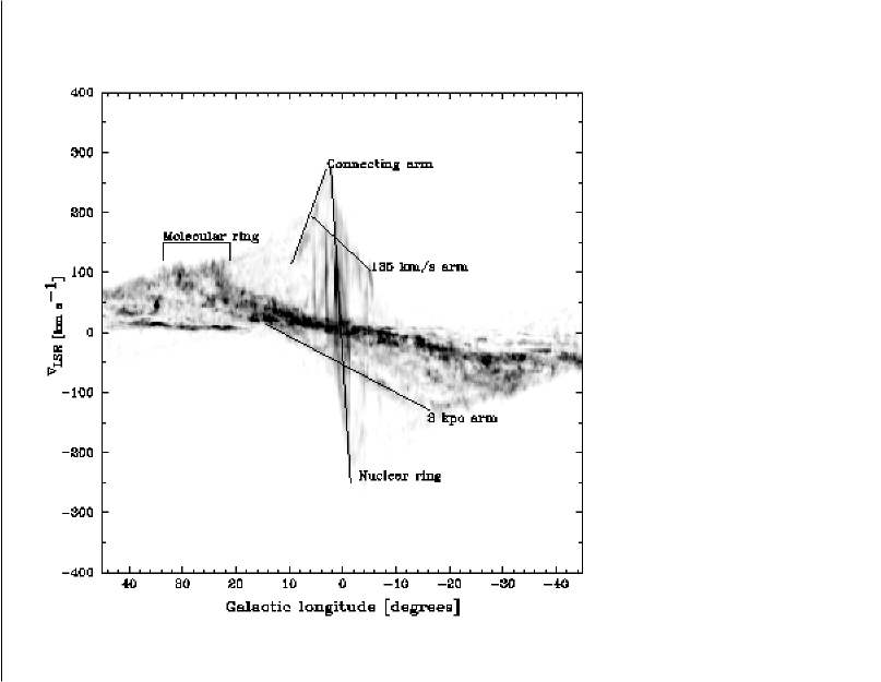
Figure 4: CO ($l,v$) diagram from Dame et al. (2001). Gas features are labelled as in Fig. 1 of Fux (1999).

The centre of our Galaxy contains a massive black hole. The advent of adaptive optics has permitted high spatial resolution imaging studies of the Galactic centre. A dense cluster of stars surrounds Sgr A, and proper motions of these stars were recently obtained, showing them to have high velocities of up to 5000 km s^-1. Thereby the mass of the central black hole has been estimated to be ($3.3\pm 0.7)\times 10^{6}$ M_⊙ (e.g. Schödel et al. 2003; Ghez et al. 2000). Massive star formation is still going on in the central parsec of the Galaxy.

1 Stellar line of sight velocity surveys and the importance of maser surveys

Though the AGB phase is very short ($\sim 10^{6}$ yr) and therefore AGB stars are rare among stars, they are representative of all low and intermediate mass stars, i.e. of the bulk of the Galactic population. They are evolved stars and therefore dynamically relaxed and their kinematics traces the global Galactic gravitational potential. Thermally pulsing AGB stars are surrounded by a dense envelope of dust and molecular gas. They are bright at infrared wavelengths and can be detected even throughout highly obscured regions. Furthermore, the OH and SiO maser emission from their envelopes can be detected throughout the Galaxy, providing stellar line-of-sight velocities to within a few km s^-1. AGB stars thus permit a study of the Galactic kinematics, structure and mass-distribution.

This is especially useful in the inner regions of the Galaxy where the identification of other tracers like Planetary Nebulae is extremely difficult. Observations of H$\alpha$ and [OIII] emission lines which easily reveal velocities of Planetary Nebulae are hampered by high interstellar extinction. A dynamical study of planetary nebulae ($-5$$<b<-10$) was performed by Beaulieu et al. (2000), who found that the spatial distribution of planetary nebulae agrees very well with the COBE light distribution. However, no conclusive results were found comparing the stellar kinematics properties with models of a barred Galaxy. The poor statistics was the main problem.

Performing radio maser surveys is the most efficient way to obtain line of sight velocities in the inner Galaxy. Two extensive blind surveys have been made at 1612 MHz searching for OH/IR stars in the Galactic plane ($|l|<45$, $|b|<4$), one in the South using the ATCA, and another in the North using the VLA (Sevenster et al. 1997a, b, 2001), yielding a sample of 766 compact OH-masing sources.

Searches at 43 or 86 GHz for SiO maser emission are also successful. SiO maser lines have the advantage to be found more frequently than 1612 MHz OH maser and the disadvantage that they can only be searched in targeted surveys, since the cost of an unbiased search is too high. Several 43 GHz SiO maser surveys of IRAS point sources have been conducted by Japanese groups using the Nobeyama telescope (e.g. Izumiura et al. 1999; Deguchi et al. 2000b, a). However, those surveys are not complete at low latitudes, since there IRAS suffers from confusion.

Up to day more than 1000 maser stars are known in the inner Galaxy. A kinematical analysis of Sevenster’s sample of OH/IR stars (Sevenster 1999b; Debattista et al. 2002) shows clear signs of a barred potential. However, the number of line of sight velocities is still too small to allow us an unambiguous determination of the parameters of the bar. Furthermore, although most of the Galactic mass is in stars, a stellar longitude-velocity, $(l-v)$, diagram alone is not sufficient to constrain a model of Galactic dynamics, mainly due to the dispersion velocity of stars, which smooths the various features.

Improved statistics together with additional information on the distance distribution of masing stars will notably improve the understanding of the Galactic $(l-v)$ diagram. Low latitude stars are of particular importance since their motion may contain a signature of in-plane Galactic components, e.g. the nuclear ring, and they may show better the effect of a thin bar. New targeted maser surveys in the Galactic plane are now possible using ISOGAL and MSX sources, it is this simple idea from which the work presented in this thesis originates.

3 Outline of this thesis

To increase the number of measured line of sight velocities in the inner Galaxy ($30^{\circ}<l<-30^{\circ}$, mostly at $|b|<1$), we began a survey of 86 GHz ($v=1,J=2\rightarrow 1$) SiO maser emission. In Chapter 2 we present the survey that was conducted with the IRAM 30-m telescope. Stars were selected from the ISOGAL and MSX catalogues to have colours of Mira-like stars. SiO maser emission was detected in 271 sources (a detection rate of 61%), doubling the number of maser derived line-of-sight velocities toward the inner Galaxy. I observed and detected the first line on August 26th, 2000: it was an unforgettable moment of joy!

The collection of near- and mid-infrared measurements of SiO targets allow us to study their energy distribution and determine their luminosity and mass-loss. Chapter 3 describes a compilation of DENIS, 2MASS, ISOGAL, MSX and IRAS 1–25$\mu$m photometry of the 441 late-type stars which we searched for 86 GHz SiO maser emission. The comparison between DENIS and 2MASS $J$ and $K_{\rm S}$ magnitudes shows that most of the sources are variable stars. MSX colours and the IRAS $[12]-[25]$ colour are consistent with those of Mira type stars with a dust silicate feature at 9.7 $\mu$m in emission, indicating only a moderate mass-loss rate.

Towards the inner Galaxy the visual extinction can exceed 30 magnitudes, and even at infrared wavelengths the extinction is significant. In Chapter 4 we carry out the analysis of 2MASS colour magnitude diagrams of several fields in the plane at longitudes $l$ between 0 and 30^∘ in order to obtain extinction estimates for all SiO targets. With this analysis we are also able to put new constraints on the near-infrared extinction power-law.

The luminosity of our SiO targets is derived in Chapter 5 and compared to that of a sample of OH/IR stars. We computed stellar bolometric magnitudes by direct integration under the observed energy distribution. Assuming a distance of 8 kpc for all stars within 5 from the Galactic centre we find the luminosity distribution to peak at M${}_{\mathrm{bol}}=-5$ mag, which coincides with the peak shown by OH/IR stars in the Galactic centre. We found that the main difference between SiO targets and OH/IR stars is mass loss, which is higher in OH/IR stars. This fact offers several advantages. In contrast to OH/IR stars, SiO target stars are readily detectable in the near-infrared and therefore ideal for follow-up studies to better characterise the central star.

Considerations on the kinematics of SiO targets and future work plans are reported in Chapter6.

Finally in the last Chapter (Chapter 7) I briefly describe the ISOGAL survey, which is a 7 and 15 $\mu$m survey of $\sim$16 deg² towards selected fields along the Galactic plane, mostly toward the Galactic centre. In collaboration with A. Omont (P.I.) and the ISOGAL team, I worked on the finalisation of the ISOGAL point source catalogue (Omont et al. 2003; Schuller et al. 2003). In this Chapter, I emphasise the importance of having several recent infrared surveys, such as DENIS, 2MASS, ISOGAL and MSX, in a common effort to unveil the overall structure of the Milky Way and in particular of its central and most obscured regions. These surveys require a huge amount of technical work which is of primary importance to obtain a reliable point source catalogue that can be used to perform such studies.

It is thanks to these new catalogues that the SiO maser project, i.e. the present thesis, could be performed.

Chapter 1 86 GHz SiO maser survey of late-type stars in the Inner Galaxy I. Observational data

SiO maser survey I. Observational data

M. Messineo, H. J. Habing, L. O. Sjouwerman, A. Omont, and K. M. Menten

This chapter is available at:
${\tt http://lanl.arxiv.org/abs/astro-ph/0207284}$ or
${\tt http://www.edpsciences.org/articles/aa/pdf/2002/37/aa2744.pdf}$.

Chapter 2 86 GHz SiO maser survey of late-type stars in the Inner Galaxy II. Infrared photometry

SiO maser survey II. Infrared photometry

M. Messineo, H. J. Habing, K. M. Menten, L. O. Sjouwerman and A. Omont

This chapter is available at:
${\tt http://lanl.arxiv.org/abs/astro-ph/0401262}$ or
${\tt http://www.edpsciences.org/articles/aa/full/2004/16/aa0488/aa0488.html}$.

Chapter 3 86 GHz SiO maser survey of late-type stars in the Inner Galaxy III. Interstellar extinction and colours

Interstellar extinction and colours

M. Messineo, H. J. Habing, K. M. Menten, A. Omont,
L. O. Sjouwerman and F. Bertoldi

In this article we study the interstellar extinction toward a sample of evolved late-type stars in the inner Galaxy (-4 $<l<+30$, $|b|<1$) which were searched for SiO maser emission (“SiO targets” hereafter; Messineo et al. 2002, Chapter II). The maser emission reveals the stellar line of sight velocities with an accuracy of a few km s^-1, making the maser stars ideal for Galactic kinematics studies.

The combination of the kinematic information with the physical properties of the SiO targets, e.g. their intrinsic colours and bolometric magnitudes, will enable a revised kinematic study of the inner Galaxy, revealing which Galactic component and which epoch of Galactic star formation the SiO targets are tracing.

A proper correction for interstellar extinction is of primary importance for our photometric study of the stellar population of the inner Galaxy, where extinction can be significant even at infrared wavelengths. The extinction hampers an accurate determination of the stellar intrinsic colours and bolometric magnitudes.

This is especially critical in the central Bulge region where interstellar extinction is larger than 30 visual magnitudes and the uncertainty in the stellar bolometric luminosities of evolved late-type stars is at least 1 magnitude due to the current uncertainty in the near-infrared extinction law (30%).

The available near- and mid-infrared photometry of the SiO targets from the DENIS (Epchtein et al. 1994), 2MASS (Cutri et al. 2003), ISOGAL (Omont et al. 2003; Schuller et al. 2003) and MSX (Egan et al. 1999; Price et al. 2001) surveys were already presented by Messineo et al. (2004b, Chapter III).

The corrections for interstellar extinction of the photometric measurements of each SiO target will enable us to derive the spectral energy distributions and bolometric magnitudes of the SiO targets. The bolometric magnitudes will be presented in a subsequent paper (Messineo et al. 2004a, Chapter V).

Our sample consists mainly of large-amplitude variable AGB stars (; ). The estimates of interstellar extinction toward this class of objects are complicated by the presence of a circumstellar envelope which may have various thickness. Therefore, in order to disentangle circumstellar and interstellar extinction one needs to study the dust distribution along the line of sight toward each AGB star of interest. For each SiO target we adopt the median extinction derived from near-infrared field stars (mainly giants) close to the line of sight of the target. Then the dereddened colour-colour distribution of our targets is compared to those of local Mira stars in order to iteratively improve the extinction correction and to statistically estimate the mass-loss rates of our targets.

In Sect. 1 we discuss the uncertainty of the extinction law at near- and mid-infrared wavelengths, and the consequent uncertainty of the stellar luminosities. In Sect. 2 we describe the near-infrared colour-magnitude diagrams of field stars toward the inner Galaxy and we use the latter to derive the median extinction toward each target. In Sect. 3 we review the location of Mira stars on the colour-magnitude (CMD) and colour-colour diagrams. In Sects. 4 and 5 we use the median extinction from surrounding field stars to deredden our SiO targets and we discuss their colours and mass-loss rates. The main conclusions are given in Sect. 4.H.

1 Interstellar extinction law

The composition and abundance of interstellar dust and its detailed extinction properties remain unclear, limiting the accuracy of stellar population studies in the inner Galaxy. In the following we discuss the near- and mid-infrared extinction law, in order to assess the uncertainty in the extinction correction.

1 Near-infrared interstellar extinction

Interstellar extinction at near-infrared wavelengths (1-5 $\mu$m) is dominated by graphite grains. Although for historical reasons the near-infrared extinction law is normalised in the visual, practically it is possible to derive near-infrared extinction by measuring the near-infrared reddening of stars of known colour.

Near-infrared photometric studies have shown that the wavelength-dependence of the extinction may be expressed by a power law, A_λ $\propto\lambda^{-\alpha}$, where $\alpha$ was found to range between 1.6 (Rieke & Lebofsky 1985) and 1.9 (Glass 1999; Landini et al. 1984; van de Hulst 1946).

When deriving the extinction from broad-band photometric measurements, one needs to properly account for the bandpass, stellar spectral shape, and the wavelength-dependence of the extinction. We have therefore computed an “effective extinction” for the DENIS $I$ and 2MASS $J,~{}H$ and $K_{\rm s}$ passbands, as a function of the K_S band extinction. This effective extinction was computed by reddening an M0 III stellar spectrum (Fluks et al. 1994) with a power law extinction curve and integrating it over the respective filter transmission curves. When we convolve the filter response with a stellar sub-type spectrum different from the M0 III, the effective I-band extinction slightly differs, e.g. decreasing by 3% for a M7 III spectrum (see also van Loon et al. 2003).

The K_S-band extinction A${}_{\rm K_{\rm S}}$ can then be found from

$$A_{\rm K_{\rm s}}=C_{JK}\times E(J-K_{\rm s}),$$

$$A_{\rm K_{\rm s}}=C_{HK}\times E(H-K_{\rm s}),$$

where $E(J-K_{\rm s})$ and $E(H-K_{\rm s})$ are the reddening in the $J-K_{\rm s}$ and $H-K_{\rm s}$ colour, respectively, and the $C$ are constants. These relations are independent of visual extinction and of the coefficient of selective extinction, $R_{\rm V}=A_{\rm V}/E(B-V)$, but they depend on the slope of the near-infrared power law (see Table 1). However, to provide the reader with the traditionally used ratios between near-infrared effective extinction and visual extinction, we also used the commonly adopted extinction law of Cardelli et al. (1989). Such ratios may be useful in low-extinction Bulge windows, where visual data are also available. Cardelli et al. (1989) proposed an analytic expression, which depends only on the parameter $R_{\rm V}$, based on multi-wavelength stellar colour excess measurements from the violet to 0.9$\mu$m, and extrapolating to the near-infrared using the power law of Rieke & Lebofsky (1985). We extrapolated Cardelli’s extinction law to near-infrared wavelengths using a set of different power laws. The results are listed in Table 1.

The uncertainty in the slope of the extinction law produces an uncertainty in the estimates of the near-infrared extinction of typically 30% in magnitude (see Table 1). For a K_S band extinction of A${}_{\rm K_{\rm S}}$$=3$ mag the uncertainty may be up to 0.9 mag, which translates into an uncertainty in the stellar bolometric magnitudes of the same magnitude.

In Sect. 2 we show that a power law index $\alpha=1.6$ is inconsistent with the observed colours of field giant stars toward the inner Galaxy, and that the most likely value of $\alpha$ is $1.9\pm 0.1$.

Table 1: Near-infrared effective extinction, $\langle$A$\rangle$/A${}_{V}\propto\lambda^{-\alpha},$ for various filters. A different value of $R_{\rm V}$ does not affect A${}_{\rm K_{\rm s}}/{\rm E(H-K}_{\rm s})$ and A${}_{\rm K_{\rm s}}/{\rm E(H-K}_{\rm s})$, but the slope of the extinction curve does. Our findings favour a model with $\alpha=1.9$ (see Sect. 2).

A${}_{\rm I}/{\rm A}_{\rm V}$	A${}_{\rm J}/{\rm A}_{\rm V}$	A${}_{\rm H}/{\rm A}_{\rm V}$	A${}_{\rm K_{S}}/{\rm A}_{\rm V}$	A${}_{\rm K_{S}}/{\rm E(J-K}_{\rm s})$	A${}_{\rm K_{\rm s}}/{\rm E(H-K}_{\rm s})$	$\alpha$	RV	Ref.
0.592	0.256	0.150	0.089	0.533	1.459	1.85		Glass (1999)
0.584	0.270	0.165	0.103	0.617	1.661	1.73	3.08	He et al. (1995)
0.482	0.282	0.175	0.112	0.659	1.778	1.61	3.09	Rieke & Lebofsky (1985)
0.606	0.287	0.182	0.118	0.696	1.842	1.61	3.10	Cardelli et al. (1989)
0.563	0.259	0.164	0.106	0.696	1.842	1.61	2.50∗	”
0.606	0.277	0.169	0.106	0.623	1.684	1.73	3.10	Cardelli et al. (1989)+
0.563	0.249	0.152	0.096	0.623	1.684	1.73	2.50	”
0.606	0.267	0.158	0.096	0.561	1.548	1.85	3.10	”
0.563	0.240	0.142	0.086	0.561	1.548	1.85	2.50	”
0.606	0.263	0.153	0.092	0.537	1.496	1.90	3.10	”
0.563	0.237	0.138	0.083	0.537	1.496	1.90	2.50	”
0.606	0.255	0.144	0.084	0.493	1.401	2.00	3.10	”
0.563	0.229	0.130	0.076	0.494	1.400	2.00	2.50	”
0.606	0.238	0.127	0.070	0.420	1.236	2.20	3.10	”
0.563	0.213	0.114	0.063	0.420	1.236	2.20	2.50	”

• recent determination toward the Bulge (e.g. Udalski 2003).

• parametric expression modified to extrapolate to $\lambda>0.9~{}\mu$m with $\lambda^{-\alpha}$.

2 Mid-infrared interstellar extinction

Mid-infrared extinction (5-25 $\mu$m) is characterised by the 9.7 and 18 $\mu$m silicate features. The strength and profile of these features are uncertain and appear to vary from one line of sight to another. In the inner Galaxy silicate grains may be more abundant due to the outflows from oxygen-rich AGB stars. Another uncertainty is the minimum of $A_{\lambda}/A_{2.12}$ at 7$\mu$m, which is predicted for standard graphite-silicate mixes, though not observed to be very pronounced toward the Galactic Centre (Lutz et al. 1996; Lutz 1999).

Table 2: Effective extinction, $\langle$A$\rangle$/A${}_{K_{S}}$, using M-giant spectra (Fluks et al. 1994), for different bands defined by the ISOCAM and MSX filters (see Fig. 1). $A_{K_{S}}/A_{2.12}=0.97$.

Filter	$\lambda_{\rm ref}$	$\Delta\lambda$	Curve 1 (Mathis)	Curve 2	Curve 3 (Lutz)
			($A_{9.7}/A_{2.12}=0.54$)	($A_{9.7}/A_{2.12}=1.00$)	($A_{9.7}/A_{2.12}=1.00$ & no minimum)
	$\mu$m	$\mu$m	$\langle$A$\rangle$/A${}_{K_{S}}$	$\langle$A$\rangle$/A${}_{K_{S}}$	$\langle$A$\rangle$/A${}_{K_{S}}$
LW2	6.7	3.5	0.21	0.21	0.41
LW5	6.8	0.5	0.18	0.15	0.41
LW6	7.7	1.5	0.21	0.26	0.43
LW3	14.3	6.0	0.18	0.34	0.34
LW9	14.9	2.0	0.14	0.29	0.29
A	8.28	4.0	0.26	0.38	0.55
C	12.1	2.1	0.25	0.49	0.49
D	14.6	2.4	0.14	0.29	0.29
E	21.3	6.9	0.17	0.41	0.41

The commonly adopted mid-infrared extinction curve is that of Mathis (1990), which is a combination of a power law and the astronomical silicate profile from Draine & Lee (1984), with $A_{9.7}/A_{2.2}\simeq 0.54$ – a value found in the diffuse interstellar medium toward Wolf-Rayet stars (e.g. Mathis 1998, and references therein). However, using hydrogen recombination lines, Lutz (1999) found $A_{9.7}/A_{2.2}\simeq 1.0$ in the direction of the Galactic centre, and analysing the observed H₂ level populations toward Orion OMC-1, Rosenthal et al. (2000) derived $A_{9.7}/A_{2.12}=1.35$. It seems that the mid-infrared extinction law is not universal.

In order to derive the extinction ratios for all ISOGAL and MSX filters (for definitions see Blommaert et al. 2003; Price et al. 2001), and to analyse the effect of an increase of the depth of the 9.7 $\mu$m silicate feature on the extinction ratios, we built a set of extinction curves with different silicate peak strengths at 9.7 $\mu$m. We use a parametric mid-infrared extinction curve given by Rosenthal et al. (2000), where the widths of the 9.7 and 18 $\mu$m silicate features are those calculated by Draine & Lee (1984) and the depth of the 18 $\mu$m feature is assumed to be 0.44 times that of the 9.7 $\mu$m feature. Using this parametric fit we constructed two different extinction curves with $A_{9.7}/A_{2.2}$ equal to 1.0, one in combination with the minimum predicted by the models at 4-8 $\mu$m (Curve 2) and one without it as suggested by Lutz (1999) (Curve 3). The two curves are shown together with the Mathis curve (Curve 1, $A_{9.7}/A_{2.2}=0.54$) in Fig. 1.

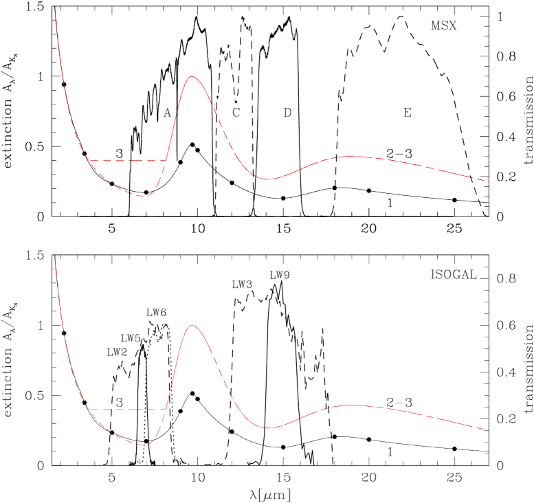
Figure 1: Filter transmission curves and extinction laws as function of wavelength. The continuous line shows the curve (Curve 1) obtained by fitting the values (dots) given by Mathis (1990); the dashed curve shows the parametric expression given by Rosenthal et al. (2000) plotted using a value of the silicate peak $A_{9.7}/A_{2.12}=1.0$ (Curve 2). The latter is also shown without the minimum around 4-8 $\mu$m (Curve 3), following Lutz (1999). In the top panel the transmission curves of the MSX $A,C,D$ and $E$ filters are also overplotted, while in the bottom panel the transmission curves of the ISOCAM $LW2,LW3,LW5,LW6$ and $LW9$ filters used in the ISOGAL survey are shown.

Using the various extinction curves detailed in Table 2, we reddened the M-type synthetic spectra from Fluks et al. (1994) (beyond 12.5$\mu$m a blackbody extrapolation is used), and convolved the resulting spectra with the ISOCAM and MSX filter transmission curves. The effective extinctions $\langle A\rangle$/A${}_{\rm K_{\rm S}}$ in the various ISOCAM and MSX filters are listed in Table 2. They are not sensitive to the stellar sub-type used. An increase of the ratio $A_{9.7}/A_{2.2}$ from 0.54 to 1.0 results in an increase between 0.15 and 0.20$\times$A${}_{\rm K_{\rm S}}$ of the average attenuation in the $LW3,~{}LW9,~{}C,~{}D$ and $E$ spectral bands. The spectral bands of the $LW2$ and $LW5$ filters are not very sensitive to the intensity of the silicate feature, but to the minimum of the extinction curve in the 4-8 $\mu$m region. Although $\langle A\rangle$/A${}_{\rm K_{\rm S}}$ varies with A${}_{\rm K_{\rm S}}$, these variations are small compared to those arising from different choices of the mid-infrared extinction law.

Hennebelle et al. (2001) obtained observational constraints on mid-infrared extinction ratios from observations of infrared dark clouds within the ISOGAL survey. Using observations in the $LW2$ and $LW3$ bands in the inner Galactic disk they obtained $A_{\rm LW2}/A_{\rm LW3}=0.7$, and using observations in the two bands $LW6$ and $LW9$ in the region ($|l|<1^{\circ},~{}0.2^{\circ}<|b|<0.4^{\circ}$) they found $A_{\rm LW6}/A_{\rm LW9}=0.8$. Both these values are in good agreement with the extinction curve calculated by Draine & Lee (1984) with a silicate peak at 9.7 $\mu$m of 1.0 (Curve 2 in Table 2). However, for the clouds located at ($|l|<1^{\circ},|b|<0.2^{\circ}$) observed in the $LW5$ and $LW9$ bands Hennebelle et al. (2001) found $A_{\rm LW5}/A_{\rm LW9}=1.07$, which is twice the value predicted by Curve 2 in Table 2, but would be consistent with Curve 1 or 3.

For stars in the inner disk Jiang et al. (2003) derived (A${}_{\rm K_{\rm S}}$$-A_{\rm LW2})/(A_{\rm J}-$A${}_{\rm K_{\rm S}}$) $=0.35$ and (A${}_{\rm K_{\rm S}}$$-A_{\rm LW3})$ $/(A_{\rm J}-$A${}_{\rm K_{\rm S}}$) $=0.39$. These ratios when combined with the near-infrared extinction law imply that $A_{\rm LW2}/$A${}_{\rm K_{\rm S}}$ must range from 0.35 to 0.47 and $A_{\rm LW3}/$A${}_{\rm K_{\rm S}}$ from 0.28 to 0.41, which are higher values than those produced by Curve 1 and suggest an attenuation of the minimum at 4-8 $\mu$m, consistent with Curve 3.

Concluding, there is some uncertainty in the mid-infrared extinction law that is in part due to uncertainties in the photometric measurements and possibly due to spatial variations in the strength of the silicate features. In the most obscured regions (A${}_{\rm K_{\rm S}}$$=3$) uncertainties for the ISOGAL and MSX filters range from 0.45 mag ($LW3,LW9,D$) to 0.85 mag ($A$). However, this has a negligible effect (0.1 mag in average) on the calculated $M_{\mathrm{bol}}$ of the SiO targets because their energy is emitted mostly at near-infrared wavelengths, and has therefore also a negligible effect on the mass-loss rate estimates (see Sect. 5).

In the following we will use the Lutz law (Curve 3) to deredden the colours of our SiO targets, since this law ensures a consistency between mid-infrared and near-infrared stellar colours as found by Jiang et al. (2003).

2 Interstellar extinction of field stars from near-infrared colour-magnitude diagrams

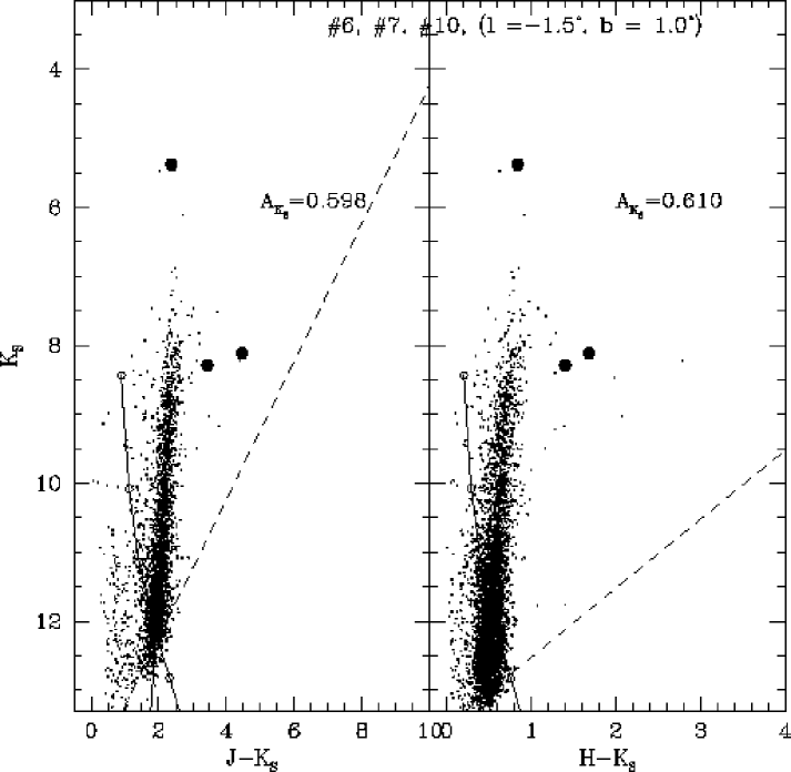
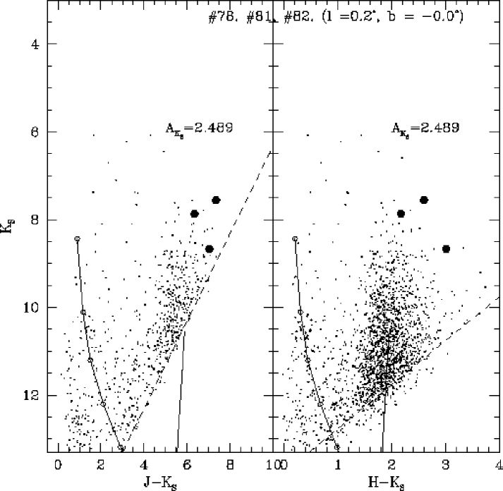
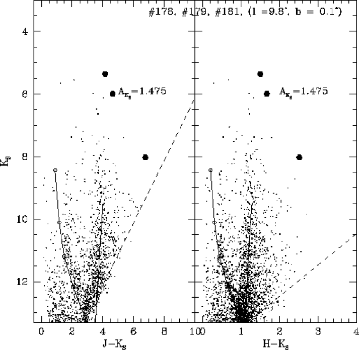
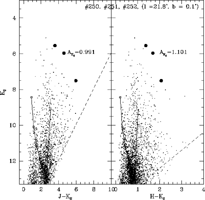
Figure 2: Colour-magnitude diagrams of 2MASS datapoints (small dots) of good quality located within 4 from the position of the SiO target (big dot). Three fields at equal median extinction are combined in each panel. The right-hand continuous line indicates the locus of the reference RGB curve (see Sect. 1), adopting a distance of 8 kpc and reddening it with the median extinction of field stars (A${}_{\rm K_{\rm S}}$). The left-hand continuous curve shows the trace of clump stars for increasing distance and extinction along a given line of sight (see Sect. 3), obtained using the extinction model by Drimmel et al. (2003) and the absolute magnitudes from Wainscoat et al. (1992). Dashed lines indicate the diagonal cut-offs due to the detection limits in $J$ and $H$. Circles on the clump trace mark a distance from 1 to 5 kpc with a step of 1 kpc downward.

Most of the sources detected by DENIS and 2MASS toward the inner Galaxy are red giants and asymptotic giant branch stars. Because the intrinsic $(J-K_{S})_{0}$ colours of giants are well known and steadily increase from 0.6 to 1.5 mag with increasing luminosity, one can study the colour-magnitude diagrams (CMDs) of $(J-K_{\rm s})$ versus $K_{\rm s}$ and of $(H-K_{\rm s})$ versus $K_{\rm s}$ to estimate the average extinction toward a given line of sight for a population of such stars.

Under the assumption that our SiO targets are spatially well mixed with the red giant stars, and that the interstellar extinction is uniform over a 4$\times 4$ field (corresponding to 9$\times$9 pc² at the distance of the Galactic Centre), we estimate the extinction, A${}_{\rm K_{\rm S}}$, towards our 441 SiO targets by examining the CMDs of 2MASS sources in field of 2-4 radius around each SiO target. Figure 2 shows a representative sample of these CMDs. We assume that the red giant branch (RGB) has the same intrinsic shape for all red giants in the inner Galaxy: the absolute magnitude of the tip of the RGB, $M_{\rm K_{\rm s}}(tip)$, and the RGB colour-magnitude relation does not vary. This means that at a given distance, $d$, along the line of sight the observed RGB extends towards fainter magnitudes from the tip at magnitude $K_{\rm s}(tip)=M_{\rm K_{\rm s}}(tip)+DM+A_{\rm K_{\rm s}}$; here $DM$ is the distance modulus corresponding to $d$ and A${}_{\rm K_{\rm S}}$ the corresponding extinction in the K_S band. With increasing distance along a given line of sight the RGB becomes redder, due to the increase of interstellar extinction. The reddening is proportional to the extinction, A${}_{\rm K_{\rm S}}$, and the shift to fainter magnitudes equals $DM+$A${}_{\rm K_{\rm S}}$. In principle we could thus derive both $DM$ and A${}_{\rm K_{\rm S}}$ as a function of distance by locating discrete features of the RGB. Due to small number fluctuations, it is difficult to estimate $K_{\rm s}(tip)$ and thus $DM+$A${}_{\rm K_{\rm S}}$. Some of the CMDs contain also the so-called “red clump” stars which all have the same absolute magnitude ($M_{\rm K_{\rm s}}=-1.65$), so that they can be used to trace the stellar distribution and that of the dust along the line of sight. However, close to the Galactic centre the distance modulus and the extinction shift clump stars below the detection limits of DENIS and 2MASS.

The average field extinction can be estimated by assuming a reference isochrone (colour-magnitude relation) for the RGB (Sect. 1), and by fitting the isochrone to the observed giants. This approach was used by Schultheis et al. (1999) and Dutra et al. (2003) to map the extinction in the central region of the Galaxy ($|l|<10$). Schultheis et al. (1999) obtained an extinction map within 8^∘ of the Galactic Centre by comparing DENIS ($J,K_{\rm s}$) photometry with an isochrone from Bertelli et al. (1994) (metallicity $Z=0.02$, age 10 Gyr, distance 8 kpc), adopting the extinction law of Glass (1999). A similar map was also produced by Dutra et al. (2003) using 2MASS ($J,K_{\rm s}$) data together with an empirical reference RGB isochrone, which is a linear fit to the giants in Baade’s windows, and adopting the extinction law of Mathis (1990).

The SiO targets are located at longitudes $l$ between 0 and 30 and mostly at latitude $b<0.5^{\circ}$. In this region of high extinction even at near-infrared wavelengths, fits to the apparent (K_S, $J-$K_S) RGB may underestimate the extinction, due to observational bias as explained in Sect. 2 (see also Dutra et al. 2003; Cotera et al. 2000; Figer et al. 2004). Therefore it is useful to also consider the (K_S, $H-$K_S) plane, which is deep and not sensitive to extinction and therefore less affected by bias.

The extinction toward each of the SiO targets was calculated from individual field stars in both the (K_S, $J-$K_S) and (K_S, $H-$K_S) CMDs by shifting the datapoints on the reference RGB (see Sect. 1) along the reddening vector. Then, the median extinction of the field was determined in both the (K_S, $J-$K_S) and (K_S, $H-$K_S) planes, applying an iterative 2$\sigma$ clipping to the extinction distribution in order to exclude foreground stars (Dutra et al. 2003). A comparison of the extinction estimates derived from both diagrams, and possible selection effects are described in Sect. 2.

SiO targets usually appear redder than neighbouring stars (Fig. 2), which implies that they are intrinsically obscured if we assume that the spatial distribution of SiO targets is the same as that of red giant branch stars. About fifty of our 441 SiO target stars are brighter in K_S and bluer than sources in the field, so those must be nearer than the median.

The CMDs contain much information on the distribution of stars and dust in the inner Galaxy. Here we have used them only to estimate a median extinction, A${}_{\rm K_{\rm S}}$. In a future study we hope to make a more complete analysis of these diagrams with a more self-consistent model. In the following some general remarks from the analysis of the CMDs are summarised:

• We can determine A${}_{\rm K_{\rm S}}$ for individual stars in each CMD and the statistical properties of the extinction values within a given CMD. In most CMDs the interstellar extinction, A${}_{\rm K_{\rm S}}$, shows a strong concentration, which reflects the Bulge and the Galactic centre. In a minority of CMDs the histogram is broad without clear peaks.

• Broad, diffuse extinction distributions are found at longitudes 20$<l<$ 30. This suggests that stars and dust are spread along these line of sight.

• Lines of sight which pass through complex star forming regions such as M17 are easily identified as regions of anomalously high extinction compared to their surrounding regions.

• Toward some lines of sight, especially at latitudes above $|b|\approx$ 0.6 , a sharp edge at the high end is found in the extinction distribution. These lines of sight apparently extend to above the dust layer.

Table 3: Extinction values. The identification number (ID) of the SiO target, as in Table 2 and 3 of Chapter II, is followed by the field extinction A${}_{\rm K_{\rm S}}$, by the corresponding dispersion of individual extinctions of field stars, and by the total extinction in K_S-band toward the target star (tot). Finally, a flag (Fg) is listed, which is equal to unity when the SiO target is classified as a “foreground object”. Stars for which not all $J,H,$K_S measurements were available have no total extinction.

ID	A${}_{\rm K_{\rm S}}$	$\sigma_{\rm A_{\rm K_{\rm S}}}$	tot	Fg	ID	A${}_{\rm K_{\rm S}}$	$\sigma_{\rm A_{\rm K_{\rm S}}}$	tot	Fg	ID	A${}_{\rm K_{\rm S}}$	$\sigma_{\rm A_{\rm K_{\rm S}}}$	tot	Fg	ID	A${}_{\rm K_{\rm S}}$	$\sigma_{\rm A_{\rm K_{\rm S}}}$	tot	Fg
	mag	mag	mag			mag	mag	mag			mag	mag	mag			mag	mag	mag
1	0.96	0.18	1.63		61	1.72	0.29	3.46		121	1.65	0.28	1.91		181	1.38	0.59	2.77
2	1.23	0.31	2.81		62	1.70	0.28	2.47		122	1.55	0.25	2.10		182	1.29	0.19	1.46
3	1.90	0.33	1.79		63	2.44	0.42	3.18		123	1.26	0.36	1.51		183	1.32	0.28	1.45
4	2.16	0.52	3.00		64	2.28	0.42	3.67		124	1.43	0.30	2.18		184	1.44	0.29	1.62
5	1.51	0.25	1.75		65	2.28	0.42	3.67		125	1.65	0.35	2.26		185	1.37	0.24	0.44	1
6	0.59	0.09	1.16		66	1.71	0.21	1.21	1	126	0.75	0.11	1.59		186	1.57	0.18	1.51
7	0.57	0.07	0.51		67	1.62	0.26	2.09		127	0.91	0.19	1.78		187	0.97	0.33	1.65
8	1.98	0.41	1.53	1	68	1.68	0.23	1.09	1	128	1.51	0.24	1.60		188	0.85	0.22	1.06
9	2.14	0.32	2.59		69	2.17	0.43	2.53		129	0.93	0.24	0.36	1	189	0.21	0.04	1.14
10	0.61	0.11	1.48		70	1.65	0.36	2.02		130	0.79	0.09	0.52	1	190	1.04	0.59	1.10
11	0.94	0.17	1.04		71	1.84	0.35	2.12		131	1.69	0.44	1.94		191	2.22	0.75	3.39
12	1.21	0.17	1.61		72	1.86	0.23	2.24		132	1.61	0.42	2.53		192	0.93	0.33	1.69
13	1.11	0.23	2.15		73	2.63	0.30	3.94		133	0.99	0.19	0.86		193	0.97	0.34	1.60
14	1.38	0.14	1.66		74	1.42	0.18	1.92		134	1.52	0.26	2.60		194	1.37	0.20	1.94
15	1.34	0.27	0.89	1	75	1.36	0.23	1.19		135	1.20	0.27	1.46		195	1.42	0.14	1.71
16	1.46	0.15	1.99		76	2.71	0.38	3.58		136	1.27	0.13	1.48		196	1.85	0.79	2.84
17	1.45	0.15	1.86		77	2.49	0.43	2.22		137	1.21	0.24	1.73		197	1.91	0.53	2.02
18	1.53	0.27	1.89		78	2.49	0.43	3.74		138	1.11	0.19	2.17		198	1.76	0.47	2.46
19	0.60	0.06	0.71		79	1.88	0.34	1.93		139	0.21	0.04	0.95		199	1.22	0.31	0.57	1
20	1.47	0.21	1.81		80	2.12	0.28	2.81		140	1.03	0.13	0.38	1	200	2.10	1.07	1.97
21	1.40	0.29	1.35		81	2.53	0.38	2.56		141	1.22	0.17	2.49		201	0.92	0.24	1.49
22	1.40	0.29	1.82		82	2.45	0.40	3.33		142	1.22	0.16	1.26		202	0.92	0.24	0.14	1
23	1.73	0.63	1.06	1	83	1.58	0.23	1.50		143	1.30	0.19	1.96		203	0.91	0.26	3.15
24	2.17	0.36	3.07		84	2.34	0.39	2.90		144	1.49	0.32	1.36		204	0.97	0.25	3.04
25	1.83	0.26	1.10	1	85	2.24	0.44	2.25		145	1.02	0.18	0.98		205	1.19	0.32	1.46
26	2.26	0.40	2.73		86	2.21	0.68	2.88		146	0.83	0.15	1.06		206	2.36	0.48	0.45	1
27	1.93	0.24	2.19		87	1.69	0.14	1.24	1	147	1.34	0.27	0.89	1	207	1.15	0.29	1.17
28	2.09	0.36	2.77		88	2.45	0.51	3.07		148	0.80	0.21	0.57	1	208	0.91	0.33	1.41
29	2.56	0.32	4.31		89	2.60	0.41	2.97		149	1.17	0.25	1.43		209	1.91	0.63	2.70
30	2.82	0.36	3.92		90	1.90	0.34	2.12		150	1.33	0.31	2.23		210	0.88	0.24	1.64
31	1.80	0.19	1.72		91	2.82	0.52	3.09		151	1.17	0.32	1.41		211	1.42	0.53	2.50
32	1.61	0.24	1.78		92	1.66	0.28	1.40		152	1.08	0.39	1.88		212	0.82	0.31	2.02
33	1.62	0.22	2.69		93	1.87	0.35	1.85		153	0.14	0.15	0.34		213	2.56	1.05	4.03
34	1.78	0.25	2.67		94	2.07	0.47	3.62		154	1.73	0.64	5.16		214	1.00	0.19	1.13
35	1.89	0.23	2.50		95	2.11	0.76	4.65		155	1.20	0.30	1.55		215	1.30	0.36	3.56
36	1.47	0.22	0.80	1	96	1.92	0.32	1.88		156	0.97	0.25	1.75		216	0.89	0.35	1.43
37	1.87	0.25	3.37		97	2.31	0.61	3.38		157	1.31	0.33	1.42		217	1.02	0.34	1.89
38	2.98	0.44	3.52		98	2.37	0.61	2.94		158	1.42	0.32	1.60		218	1.30	0.65	1.40
39	2.91	0.44	3.64		99	2.41	0.56	2.34		159	1.46	0.19	2.15		219	1.48	0.31	2.15
40	2.29	0.35	2.79		100	2.30	0.56	3.55		160	1.35	0.23	0.81	1	220	2.21	0.57	3.39
41	2.68	0.40	3.53		101	2.11	0.39	3.89		161	1.84	0.35	2.12		221	1.10	0.35	2.24
42	2.19	0.41	2.37		102	2.24	0.48	2.24		162	1.66	0.41	3.35		222	1.93	0.37	2.29
43	1.66	0.26	3.29		103	0.99	0.16			163	1.75	0.47	2.25		223	1.02	0.29	1.87
44	1.75	0.21	1.86		104	0.92	0.10	1.21		164	1.32	0.30	1.49		224	2.04	0.57
45	2.67	0.34	3.76		105	1.62	0.31	2.32		165	1.08	0.21	2.67		225	1.53	0.48	2.24
46	2.89	0.47	4.44		106	1.23	0.54	2.10		166	1.21	0.26	2.44		226	0.84	0.28	1.10
47	1.34	0.11	1.15	1	107	1.70	0.42	2.56		167	1.26	0.18	1.58		227	1.83	0.26	0.61	1
48	2.25	0.39	2.67		108	2.01	0.56	0.77	1	168	1.35	0.16	1.52		228	0.92	0.32	1.94
49	2.33	0.41	2.69		109	1.88	0.39	2.98		169	1.11	0.48	1.98		229	1.32	0.43	2.29
50	1.10	0.16	1.75		110	1.78	0.53	2.64		170	1.19	0.19	1.96		230	0.87	0.26	1.61
51	2.31	0.39	3.70		111	1.81	0.38	2.10		171	1.57	0.31	1.67		231	0.70	0.22	1.54
52	2.33	0.38	3.86		112	1.35	0.30	1.32		172	1.09	0.33	2.79		232	1.10	0.35	1.45
53	2.68	0.34	2.65		113	1.70	0.28	1.14	1	173	1.61	0.63	1.20		233	1.64	0.54	1.56
54	2.31	0.38	2.33		114	1.25	0.28	1.47		174	1.02	0.53	1.49		234	1.18	0.38	2.17
55	1.71	0.27	2.94		115	1.92	0.43	2.00		175	1.20	0.39	2.09		235	1.00	0.36	1.77
56	2.34	0.36	2.49		116	1.75	0.46	1.41		176	1.42	0.50	1.46		236	0.81	0.30	1.90
57	2.55	0.45	3.49		117	1.85	0.41	3.25		177	1.27	0.30	1.51		237	0.75	0.23	2.00
58	2.20	0.33	3.59		118	2.78	0.59	3.97		178	1.50	0.37	1.48		238	0.95	0.37	1.34
59	2.25	0.34	2.38		119	1.63	0.60	1.54		179	1.43	0.32	1.79		239	0.83	0.30	1.49
60	2.11	0.29	2.75		120	1.62	0.29	2.27		180	1.20	0.38	1.05		240	0.76	0.30	2.00

Table 3: (continued)

ID	A${}_{\rm K_{\rm S}}$	$\sigma_{\rm A_{\rm K_{\rm S}}}$	tot	Fg	ID	A${}_{\rm K_{\rm S}}$	$\sigma_{\rm A_{\rm K_{\rm S}}}$	tot	Fg	ID	A${}_{\rm K_{\rm S}}$	$\sigma_{\rm A_{\rm K_{\rm S}}}$	tot	Fg	ID	A${}_{\rm K_{\rm S}}$	$\sigma_{\rm A_{\rm K_{\rm S}}}$	tot	Fg
	mag	mag	mag			mag	mag	mag			mag	mag	mag			mag	mag	mag
241	0.92	0.29	2.05		301	2.13	0.33	1.88		361	1.60	0.49	3.67		421	1.06	0.45	3.64
242	0.88	0.20	0.93		302	2.56	0.33	2.50		362	1.35	0.18			422	1.25	0.44	1.86
243	0.92	0.32	2.42		303	1.36	0.11	0.63	1	363	1.87	0.41	3.00		423	0.72	0.68	0.32
244	0.96	0.39	0.99		304	2.07	0.35	3.41		364	0.61	0.09	0.96		424	1.34	0.40	2.28
245	0.67	0.22	0.89		305	1.79	0.22	2.53		365	1.72	0.26	3.62		425	1.72	0.71	1.37
246	1.15	0.44	1.65		306	1.88	0.24	2.06		366	0.60	0.15	1.21		426	1.07	0.47	2.53
247	1.26	0.36	0.79	1	307	1.24	0.13	1.48		367	1.16	0.32	2.95		427	0.90	0.46
248	1.26	0.39	1.61		308	2.20	0.36	2.92		368	1.57	0.31	0.63	1	428	0.94	0.41	1.53
249	0.98	0.42	2.31		309	2.26	0.35	2.52		369	1.35	0.22	2.58		429	0.74	0.39	1.70
250	0.93	0.42	2.36		310	2.79	0.41	2.42		370	1.11	0.23	0.53	1	430	0.88	0.32	1.63
251	1.39	0.42	1.74		311	2.93	0.51	4.32		371	0.83	0.14	1.49		431	0.83	0.31	1.17
252	0.92	0.31	1.23		312	1.70	0.28	2.14		372	1.24	0.16	2.13		432	0.97	0.35	1.17
253	0.96	0.32	2.34		313	1.75	0.28	2.25		373	1.24	0.11	1.12	1	433	0.72	0.29	1.84
254	1.27	0.55	1.82		314	2.18	0.46	3.18		374	0.95	0.20	1.36		434	1.71	0.60	1.84
255	1.13	0.30	1.22		315	1.05	0.13	1.47		375	1.03	0.21	1.70		435	1.02	0.45	0.40	1
256	0.84	0.61	2.80		316	1.54	0.22	1.77		376	1.33	0.22	2.97		436	0.97	0.36	0.00	1
257	0.90	0.38	4.34		317	1.32	0.15	1.53		377	1.11	0.22	1.80		437	1.01	0.34	3.31
258	1.64	0.70	2.88		318	1.63	0.25	2.15		378	0.80	0.24	1.00		438	0.99	0.30	0.38	1
259	0.85	0.48	1.07		319	0.61	0.08	1.16		379	0.84	0.19	0.68		439	0.99	0.34	2.42
260	1.08	0.43	1.67		320	2.20	0.33	2.60		380	1.03	0.31	2.52		440	1.03	0.32	0.45	1
261	1.62	0.37	2.44		321	2.28	0.43			381	1.79	0.55	2.60		441	1.02	0.44	1.34
262	1.45	0.34	1.71		322	2.23	0.41	3.79		382	0.86	0.16	0.95		442	1.17	0.53	2.69
263	0.91	0.49	1.80		323	1.87	0.25	2.92		383	1.13	0.31	1.52		443	0.96	0.57
264	1.11	0.36	1.78		324	2.41	0.49	3.49		384	1.33	0.35	0.86	1	444	1.16	0.70	0.88
265	0.84	0.33	1.48		325	2.13	0.43	2.08		385	1.17	0.39	1.67
266	0.75	0.30	1.52		326	1.74	0.21	2.62		386	1.61	0.20	1.23	1
267	0.72	0.34	1.04		327	2.17	0.25	3.09		387	2.00	0.55	5.02
268	0.74	0.30	2.59		328	1.39	0.21	1.95		388	1.77	0.56	3.17
269	0.82	0.30	1.32		329	1.74	0.24	2.06		389	1.28	0.23	2.15
270	0.88	0.31	2.22		330	1.90	0.28	2.59		390	1.56	0.32	1.36
271	1.00	0.54	2.46		331	2.15	0.27	3.22		391	1.58	0.31	2.36
272	1.48	0.30	1.51		332	2.58	0.37	2.89		392	1.39	0.29	2.19
273	1.80	0.45			333	2.41	0.44	3.12		393	0.75	0.19	1.39
274	0.49	0.05	0.96		334	2.59	0.45	2.27		394	1.16	0.46	2.31
275	0.47	0.05	0.40	1	335	2.33	0.52	2.13		395	0.92	0.22	0.63	1
276	2.27	0.60	3.76		336	2.14	0.23	2.82		396	1.24	0.26	0.37	1
277	0.57	0.07	0.49	1	337	1.37	0.15	1.52		397	1.03	0.29	1.04
278	2.12	0.40	2.92		338	2.23	0.34	2.23		398	1.55	0.29	0.38	1
279	0.98	0.17	1.23		339	2.28	0.33	2.28		399	1.08	0.29	1.45
280	1.18	0.21	1.60		340	1.26	0.19	1.50		400	1.39	0.34	4.32
281	0.93	0.14	1.34		341	2.83	0.58	4.58		401	1.24	0.21	1.34
282	1.38	0.19	2.09		342	2.62	0.39	3.31		402	1.79	0.27	0.00	1
283	1.21	0.11	1.51		343	2.60	0.52	2.56		403	1.89	0.51
284	0.83	0.12	1.54		344	2.69	0.50	2.47		404	3.43	0.48	3.90
285	1.15	0.14	1.50		345	2.13	0.61	2.61		405	2.49	1.05	0.80	1
286	0.61	0.06	0.32	1	346	2.51	0.56	2.90		406	1.56	0.21	2.01
287	0.55	0.06	0.41	1	347	2.89	0.62	0.63	1	407	0.54	0.19	2.59
288	1.43	0.21	2.15		348	2.04	0.35	3.73		408	1.41	0.16	3.58
289	1.72	0.31	2.06		349	1.63	0.27	3.79		409	1.00	0.35	2.43
290	1.51	0.22	1.70		350	1.85	0.41	1.94		410	1.27	0.38	1.85
291	1.41	0.14	0.96	1	351	1.38	0.28	2.73		411	1.02	0.34	3.10
292	1.63	0.21	2.07		352	1.25	0.24	1.69		412	1.77	0.46	1.76
293	1.62	0.30	2.21		353	1.71	0.26	2.28		413	2.13	0.44	3.65
294	2.23	0.50	2.37		354	1.36	0.25	2.63		414	0.78	0.25	1.57
295	1.67	0.22	2.18		355	1.55	0.23	2.17		415	0.95	0.25
296	1.54	0.18	1.54		356	0.82	0.11	1.08		416	0.73	0.27	0.64
297	2.35	0.28	1.07	1	357	1.84	0.46	3.40		417	0.93	0.27
298	1.50	0.17			358	1.64	0.31	0.96	1	418	0.94	0.34	3.61
299	1.54	0.15	1.99		359	1.38	0.27	2.26		419	0.79	0.37	3.41
300	2.28	0.32	3.73		360	1.46	0.29	1.36		420	1.16	0.39	3.27

1 Reference red giant branch

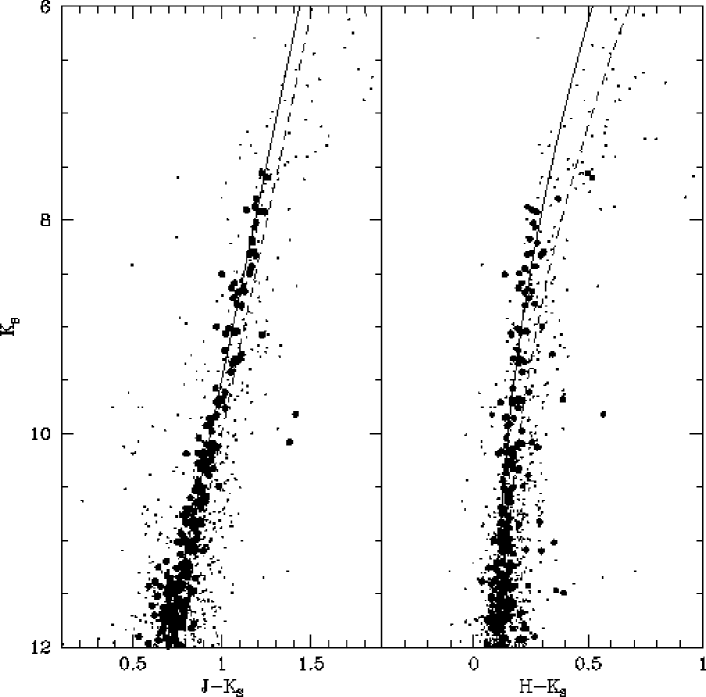
Figure 3: Magnitudes versus colours of 2MASS stars. Large dots are 2MASS sources within 4 from the centre of the globular cluster 47 Tuc, brought at the distance of 8 kpc adopting a distance modulus of 13.32 (Ferraro et al. 1999). Small dots are dereddened 2MASS Sgr–I field sources, selected within 30 from Mira stars (Glass et al. 1995) in order to overpopulate the Mira region above the RGB tip. Continuous lines indicate the mean ridge lines for the cluster red giant branch, while dashed lines those of the Sgr–I giants.

In Figure 3 we plot the extinction-corrected 2MASS point sources within 30 from the positions of Mira stars in the Sgr–I field (Glass et al. 1995). Objects above the RGB tip (K_S$\sim 8.2$ mag) are AGB stars: 63 Mira variables from (Glass et al. 1995) and 24 other stars, most probably semiregular (SR) variables (Alard et al. 2001). In the same diagram we also plot 2MASS sources within 4 from the centre of the Galactic globular cluster 47 Tuc, moved to a distance of 8 kpc (cluster distance modulus, DM=13.32 mag, from Ferraro et al. 1999).

The upper part (K_S$<12$ mag) of the 47 Tuc RGB in the $K_{\rm S0},(J-K_{\rm s})_{0}$ CMD is well represented by a linear fit:

$$({\rm J-K_{\rm s}})_{0}=2.19(\pm 0.02)-0.125(\pm 0.002){\rm K_{S0}}.$$ (1)

The 47 Tuc giants appear bluer by $0.05$ mag in $(J-K_{\rm s})_{0}$ than the colours of Sgr–I giants, which are more metal rich. However, the cluster $(J-K_{\rm s})_{0}$ vs. $K_{S0}$ RGB has a slope identical to that found in Sgr–I, confirming that the slope does not vary significantly with metallicity (see Frogel et al. 1999; Dutra et al. 2003).

To assess the uncertainty of our extinction estimates, we examined the model RGB colours of Girardi et al. (2000) with two extreme values of metallicity, Z=0.04 and 0.30. These models do not show a significant difference in the CMD slope, and they differ in $(J-K_{\rm s})_{0}$ by only 0.1 mag. A similarly small difference is found for models of 2 Gyr and 16 Gyr old populations. Nominal 2MASS photometric errors are smaller than 0.04 mag for $J<15$ and K_S$<13$ mag, but toward the Galactic centre uncertainties are larger because of crowding. However, all the uncertainties have a small impact on the extinction estimates: a change of 0.1 in $(J-K_{\rm s})_{0}$ implies a change of 0.05 in A${}_{\rm K_{\rm S}}$ (0.6 in A_V).

The right-hand panel of Fig. 3 shows the $(H-K_{\rm s})_{0}$ vs. $K_{S0}$ diagram of Sgr–I giants and of the 47 Tuc giants. There is again a well defined RGB sequence. A second order polynomial fit well fits 47 Tuc giants with K_S${}_{0}<12$ mag:

$$({\rm H-K_{\rm s}})_{0}=1.73(\pm 0.22)-0.268(\pm 0.035)\times{\rm K_{S0}}$$ (2)

$$+0.011(\pm 0.002)\times{\rm K_{S0}^{2}}.$$

At K_S${}_{0}<8$ mag this fit traces the blue boundary toward Mira stars. A fit of only Sgr–I giants is slightly more shallow:

$$({\rm H-K_{\rm s}})_{0}=2.25(\pm 0.13)-0.347(\pm 0.029)\times{\rm K_{S0}}$$ (3)

$$+0.014(\pm 0.002)\times{\rm K_{S0}^{2}}.$$

The $K_{\rm s},(H-K_{\rm s})$ plane has a lower sensitivity to extinction than the $K_{\rm s},(J-K_{\rm s})$ plane: here a colour change of 0.1 mag implies a change of $\sim 0.15$ in A${}_{\rm K_{\rm S}}$. The models of Girardi et al. (2000) predict variations within $(H-K_{\rm s})=0.04$ mag with metallicity and age variations. The nominal 2MASS photometric errors are smaller than 0.04 for $H<14$ and K_S$<13$.

The uncertainty in distance yields only a minor uncertainty in the extinction. A shift in distance modulus of the reference RGB of $\pm 2$ mag results in a change in the extinction of A${}_{\rm K_{\rm S}}$$\mp 0.15$ mag.

2 Determination of extinction value and extinction law in the $J$, $H$, $K_{\rm s}$ CMD

Assuming a colour-magnitude relation for red giants, the apparent near-infrared colours of field stars yield information on, both, the magnitude of the extinction and on the shape of the extinction law.

In principle, one can try to fit the observed field star colours to the red giant branch colours in the near-infrared colour-magnitude diagrams, and optimise the fit for both the absolute average extinction in the $K_{\rm s}$ band along the line of sight and the spectral index of the extinction power law. To do that, one needs to consider only the region of the colour-magnitude diagram where the upper RGB is well defined, i.e. not affected by large photometric errors or by the diagonal cut-off from the 2MASS detection limits (see Fig. 2), which would bias the calculation of the median extinction toward a lower value. In the inner Galaxy, the photometric error is typically below 0.04 for stars with $K_{\rm s}<12$ mag. To quantify the incompleteness due to the diagonal cut-off, with zero extinction, our average 2MASS detection limits of $J=16.0$ and $H=14.0$ correspond to a RGB K_S magnitude of 15.2 and 13.0 mag, respectively, at a distance of 8 kpc. Accounting for a scatter in the observed colours of $\pm 0.5$ mag, the RGB would be sampled well to $J=15.5$ and $H=13.5$ mag, corresponding to K_S$<14.6$ and 12.6, respectively. With a K_S extinction of 3 mag ($\sim 5.0$ mag in $H$, $\sim 8.6$ mag in $J$), a typical value in the direction of the Galactic centre, these RGB completeness limits would rise to $K_{\rm s}=7.1$ and 10.8 mag in the $(K_{\rm s},J-K_{\rm s})$ and $(K_{\rm s},H-K_{\rm S})$ planes, respectively. In the $J$ band we would therefore be left with variable AGB stars well above the RGB tip and foreground stars, and only the $H$ band would provide a sufficient number of red giant stars to match the reference RGB. We conclude from this that with the 2MASS data $(K_{\rm s},J-K_{\rm s})$ colour-magnitude diagrams are useful for extinction determinations only to a K_S extinction of about 1.6 mag, and one must always make sure that only stars above the completeness limit are matched to the RGB. Because of the larger reddening, the $(K_{\rm s},J-K_{\rm s})$ plane would in principle give more accurate extinction estimates, would it not be affected by the selection effect due to the relatively bright detection limit.

Figure 4: Comparison between the median extinction values toward our fields obtained from the (K_S,$J-$K_S) plane and those from the (K_S,$H-$K_S) plane. Only sources detected in $J,H,$K_S above the K_S completeness limits are used. In each panel a different value of the spectral index of the extinction power law, $\alpha$, is adopted.

To determine the slope, $\alpha$, of the near-infrared extinction law we examined the CMDs for field stars which were detected in all three bands, $J$, $H$, and K_S, brighter than the K_S completeness limits for the RGB at the extinction of each field. We determined the extinction toward each of our fields separately in the $(K_{\rm S},J-K_{\rm s})$ and $(K_{\rm s},H-K_{\rm s})$ CMDs, as the median of the extinctions from individual field stars. The difference of the extinction determinations from the two planes must agree independent from A${}_{\rm K_{\rm S}}$within the dispersion.

Therefore, we vary $\alpha$ until we get an overall agreement between the extinction estimates from the two planes. Figure 4 shows the differences of the median extinction values A${}_{\rm K_{\rm S}}$($J$,K_S)$-$A${}_{\rm K_{\rm S}}$($H$,K_S) plotted against the A${}_{\rm K_{\rm S}}$ -calculated- for different values of $\alpha$. The discrepancy between the extinction values increases with A${}_{\rm K_{\rm S}}$ if the assumed value of $\alpha$ is too small. We find that for $\alpha=1.9$ the two extinction estimates do yield consistent values, within the photometric uncertainties, over the entire range of A${}_{\rm K_{\rm S}}$.

The main uncertainty in the determination of the extinction power law arises from the uncertainty in the slope of the RGB. Using a fit to the colour-magnitude distribution of the giants in the Sgr–I field ($l=1.4$,b$=-2.6$) instead of the 47 Tuc globular cluster giants, that is somewhat steeper in the (K_S,$H-$K_S) plane, we find that the best value for alpha increases to 2.2.

The slope of the RGB decreases with increasing metallicity, leading to higher values of $\alpha$. However, since 47 Tuc has a lower metallicity ($-0.7$ dex) than the average Bulge stars (Frogel et al. 1999; McWilliam & Rich 1994), $\alpha=1.9$ may be taken as a lower limit to the actual value.

We furthermore find that the (K_S,$H-$K_S) distribution of the giants in the low extinction region (A${}_{\rm K_{\rm S}}$=0.2) at $l=0.2$and b$=-2.1$ (Dutra et al. 2002; Stanek 1998) match the distribution of the 47 Tuc giants better than that of Sgr–I.

Figure 5: $J-H$ vs. $H-$K_S colours. The arrows are the reddening vectors for a visual extinction of 35 mag and a near-infrared power law slopes $\alpha$ of 1.6, 1.9 and 2.0. Left-hand panel: Bulge giant stars with $10<K_{\rm s}<8$ mag taken from several Bulge fields at different median extinction. Right-hand panel: Giant stars from 47 Tuc with $10<K_{\rm s}<8$ mag when brought at the distance of the Galactic centre. The same stars are plotted again reddened using the near-infrared power laws with slope $\alpha=$ 1.6, 1.9 and 2.2 and A_K=2.9.

Although complicated by the intrinsic colour-magnitude relation that giant stars follow, the value of the $\alpha$ parameter can be tested using a $J-H$ vs. $H-$K_S diagram. Using the values from Table 1 for power laws with $\alpha=1.6$, 1.85, 1.9, 2.0, 2.2, the slopes of the reddening vector in the $J-H$ vs. $H-$K_S diagram are 1.64, 1.75, 1.80, 1.83, 1.94, respectively. Identical slopes are found when reddening artificially the 47 Tuc giants (or the Sgr–I giants) and linearly fitting the non-reddened giants plus the reddened ones. A $J-H$ vs. $H-$K_S diagram of giant stars from fields with median extinction between A${}_{\rm K_{\rm S}}$$=2.0$ and 2.3 mag and from Sgr–I field is shown in Fig. 5. The best fit to the datapoints gives a slope of $1.81\pm 0.03$, also suggesting that $\alpha=1.9\pm 0.1$.

The value $\alpha=1.9$ is in agreement with the work of Glass (1999) and Landini et al. (1984) and the historical Curve 15 of van de Hulst (1946).

In the rest of the paper we use the extinction calculated assuming $\alpha=1.9$. For fields with A${}_{\rm K_{\rm S}}$$<1.6$ mag we adopt the extinction values determined from the (K_S,$J-$K_S) plane, otherwise we will use the values from the (K_S,$H-$K_S) plane.

3 Outside the Bulge

K2 giant stars are the dominant population of late-type stars seen along the disk (e.g. Drimmel et al. 2003; López-Corredoira et al. 2002). They correspond to red clump stars in metal-rich globular clusters such as 47 Tuc. The location of clump stars on the CMD depends on extinction and distance. This trace was modelled taking the absolute magnitudes of clump stars from Wainscoat et al. (1992) and the distribution of dust and stars in the Galaxy found by Drimmel et al. (2003). The trace of the clump stars is shown by the left curve in Fig. 2, and it appears more populated by stars and distinct from the Bulge RGB in the CMD of the field at $l=\sim 10$.

Toward the Bulge the Bulge RGB population is dominant and therefore the median interstellar extinction is practically not affected by possible foreground clump stars. This is not the case in the disk, where one must eliminate the foreground clump stars before fitting the RGB in order to properly calculate the median extinction of field giants.

We therefore identified as likely clump stars those located within 0.3 mag from the $J-$K_S colour of the clump trace, and we identify as giants those stars redder than the clump stars (e.g. López-Corredoira et al. 2002).

4 Dispersion of the extinctions along a line of sight

Toward a given target star together with the median extinction of field stars A${}_{\rm K_{\rm S}}$ we determined the standard deviation of the distribution of the individual extinctions, $\sigma_{\rm A_{\rm K_{\rm S}}}$.

The patchy nature of the extinction is visible even within the $2-4\arcmin$ radius sampling area. This patchiness integrated over a longer path generates larger $\sigma_{\rm A_{\rm K_{\rm S}}}$ with increasing extinction for Bulge line of sights. The 1$\sigma_{\rm A_{\rm K_{\rm S}}}$ uncertainty in the field extinction varies from $\sim 0.2$ mag when A${}_{\rm K_{\rm S}}$$=0.6$ mag up to $\sim 0.7$ mag in the regions with the largest extinction (A${}_{\rm K_{\rm S}}$$>2.0$). In fields at longitudes longer that 10 a larger $\sigma_{\rm A_{\rm K_{\rm S}}}$ is found than in Bulge fields of similar median extinction. This is probably due to the presence of several Galactic components, e.g. the disk, arms, bar and molecular ring, along these line of sights.

3 Near-infrared properties of known Mira stars

As indicated by their variability, their strong 15 $\mu$m emission (Chapter III), and their SiO maser emission (Chapter II), our SiO targets are AGB stars in the thermal pulsing phase. At the present time their pulsation periods and amplitudes are not known. However, most of our SiO targets must be large amplitude variables (Chapter III).

Though they are 20 times less numerous than semiregular AGB stars (SRs) (Alard et al. 2001), Mira stars are among the best studied pulsating variable stars. They are regular long period variables (LPV) with visual light amplitude over 2.5 mag, or $K$ band amplitude over $\sim 0.3$ mag. Since large amplitudes tend to be associated with the most regular light curves (Cioni et al. 2003), the amplitude remains the main parameter for the classification of a Mira star.

To analyse the colours of our SiO targets, in particular to check the quality of the extinction corrections, it is useful to have a comparison sample of large amplitude LPV AGB stars, well studied and covering a wide range of colours.

Therefore, we examined various comparison samples of known Mira stars free of extinction: two samples in the solar vicinity, taken from Olivier et al. (2001) and Whitelock et al. (2000), plus one sample toward the Galactic Cap taken from Whitelock et al. (1994). To account for possible changes in the colour properties of the Mira stars with Galactic position, we also looked at two samples of Bulge Mira stars from regions of low extinction: 18 Mira stars detected by IRAS (Glass et al. 1995) in the Sgr–I field, and 104 IRAS Mira stars at latitude $6^{\circ}<b<7^{\circ}$ and $|l|<15^{\circ}$ (Whitelock et al. 1991); for comparison a sample of LPV in the Large Magellanic Cloud is also considered (Whitelock et al. 2003). All these stars have IRAS 12 $\mu$m magnitude, [12], and mean $J,H,K$ magnitudes in the SAAO system (Carter 1990).

The stellar fluxes are given already corrected for reddening only in the work of Olivier et al. (2001). For the LPV stars analysed by Whitelock et al. (2003, 2000, 1994) the effects of interstellar extinction are negligible because these stars are nearby or outside of the Galactic plane and we therefore did not correct these for extinction. We dereddened the Baade Sgr–I window data (Glass et al. 1995) adopting our favourite extinction curve ($\alpha=1.9$) and A${}_{\rm K_{\rm S}}$ $=0.15$ mag (consistently with the extinction value adopted in Glass et al. 1995). We corrected for reddening the magnitudes of the outer Bulge Miras (Whitelock et al. 1991) adopting values of A${}_{\rm K_{\rm S}}$ derived from their surrounding stars (see next section).

Next we analyse the location of these well-known Mira stars in the near-infrared CMDs and colour-colour diagrams.

1 Colour-magnitude diagram of outer Bulge Mira stars and surrounding field stars

Long period variable stars in the outer Bulge as studied by Whitelock et al. (1991) are interesting in several aspects: they were selected on the basis of their IRAS fluxes and colours according to criteria similar to those with which we selected our MSX targets (; ); since their main period ranges from 170 to 722 days and their $K$ amplitudes from 0.4 to 2.7 mag, they are classical Mira stars; their distances were estimated from the period-luminosity relation (Whitelock et al. 1991), resulting in a distribution of the distance moduli peaking at 14.7 mag with a $\sigma=\sim 0.5$ mag; since they are at latitudes between 6 and 7, they are in regions of low interstellar extinction. All this makes them ideal objects for a comparison with our SiO targets, the study of which is complicated by the large interstellar extinction at their low latitudes.

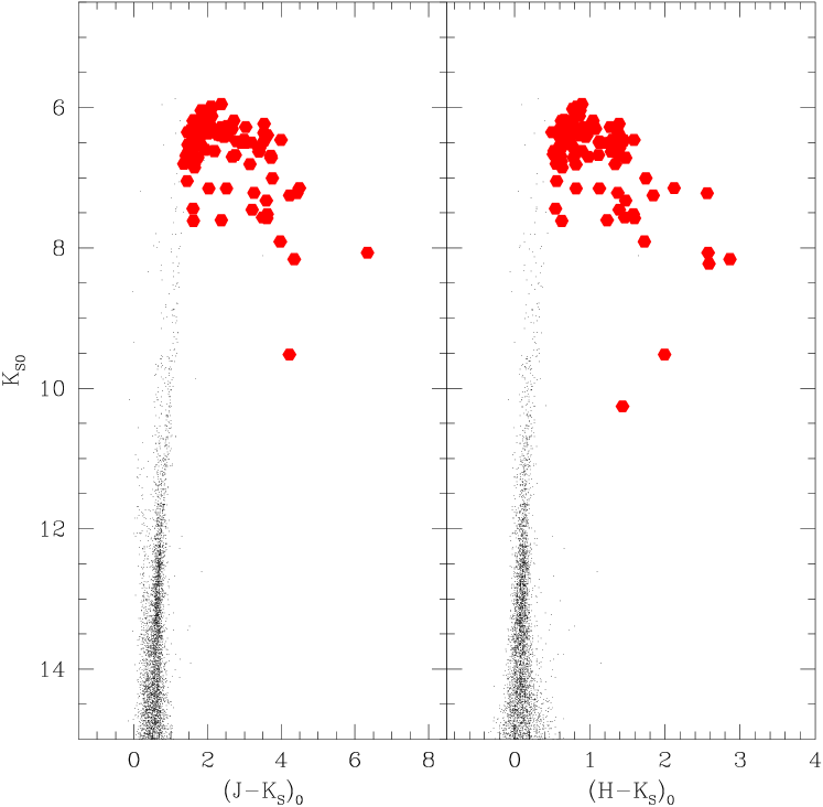
Figure 6: Dereddened colour-magnitude diagrams. Big dots represent the outer Bulge Mira stars found by Whitelock et al. (1991); the magnitudes plotted are mean magnitudes at the equal distance of 8 kpc, adopting the distances of Whitelock et al. (1991). Small dots represent the point sources detected by 2MASS within 1 from each Mira star.

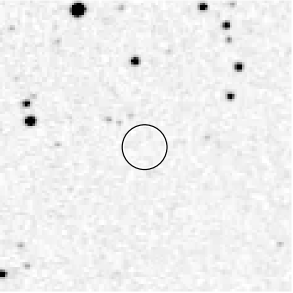
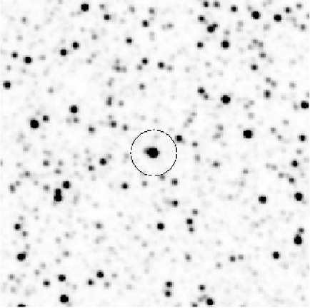
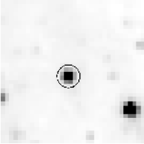
Figure 6: Op verschillende golflengten ziet de hemel er heel anders uit! Deze figuur laat hetzelfde gebied aan de hemel (afmeting 1/20^∘$\times$1/20^∘) zien op 3 verschillende golflengten. De linker afbeelding laat zien hoe het gebied in zichtbaar licht eruit ziet. Er zijn maar weinig sterren zichtbaar vanwege de hoge interstellaire extinctie. Deze foto is gemaakt met de telescoop op Mt. Palomar. De middelste afbeelding laat hetzelfde gebied zien in het nabij-infrarood; deze afbeelding is afkomstig uit de 2MASS survey. Rechts staat een ISOGAL afbeelding in het mid-infrarode deel van het spectrum. Hierin kunnen we alleen sterren zien met een circumstellaire mantel. De omcirkelde ster hebben wij gedetecteerd in onze zoektocht naar SiO maser straling (het is nr. 12 uit onze catalogus). Uit de SiO maser lijn afkomstig van deze ster hebben wij afgeleid dat deze ster zich met een snelheid van -193 km per seconde langs de gezichtslijn beweegt.

Fig. 6 shows the 2MASS point sources within 1 of each Mira star. A giant branch is clearly apparent. From an isochrone fitting (see Sect. 2) we derived the median extinction toward each field, resulting in values of A${}_{\rm K_{\rm S}}$ ranging from 0.01 to 0.30 mag, with a typical dispersion of 0.01-0.08 mag. On the colour-magnitude diagrams the Mira stars appear mostly brighter than the RGB tip of the field stars ($K=8.2$ mag at a distance of 8 kpc, see Frogel & Whitford 1987). Due to the presence of a circumstellar envelope, Mira stars have red colours (up to $(H-K_{\rm s})_{0}=3$ mag ) and lie on the red-side of the giant sequence.

It is therefore not possible to derive the interstellar extinction toward these Mira stars from their colours relative to the RGB. On the other hand, we do not have reasons to assume that the Mira stars are spatially distributed differently than the other giants stars. Therefore, the extinction of its surrounding field stars may serve as an approximation for that of the respective Mira star.

When going to lower latitude fields, however, the extinction increases and the RGB becomes broader. A worry in the assumption that a Mira star is at the median extinction of the field is the lack of knowledge of the actual distribution of extinction along the line of sight which does not warrant that the extinction of a given Mira star is the median extinction of field stars.

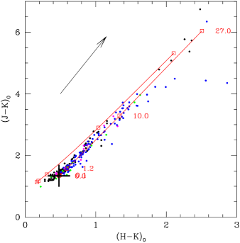
Figure 7: Dereddened colours of known dusty Mira stars (Olivier et al. 2001; Whitelock et al. 2000, 1994; Glass et al. 1995; Whitelock et al. 1991). Near-infrared mean magnitudes are used. The two curves represent M3 (upper) and an M10 (lower) type stars with increasing mass-loss rates (indicated by squares and labels $\times 10^{-6}$ M_⊙/year), as modelled by Groenewegen & de Jong (1993). The cross indicates the position of an M10 star without mass-loss ($(H-K)_{0}=0.48$ and $(J-K)_{0}=1.34$). The arrow shows the reddening vector for A_K$=1$ mag.

2 Colour-colour diagram of Mira stars

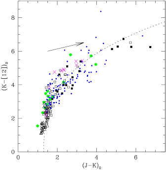
Figure 8: Dereddened colours of infrared-monitored Mira stars (based on the IRAS 12 $\mu$m and near-infrared mean magnitudes): in the solar vicinity (filled squares) (Olivier et al. 2001); detected by Hipparcos (open triangles) (Whitelock et al. 2000); toward the South Galactic Cap (open squares) (Whitelock et al. 1994); in the Baade Sgr–I window (big dots) (Glass et al. 1995); in the outer Bulge (small dots) (Whitelock et al. 1991); in the Large Magellanic Cloud (crosses) (Whitelock et al. 1994). The dotted line is the best fit to an IRAS sample of oxygen-rich AGB stars van Loon et al. (1997). The arrow shows the reddening vector for A_K$=1$ mag.

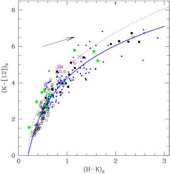
Figure 9: Dereddened colours of infrared-monitored Mira stars, based on the IRAS 12 $\mu$m and near-infrared mean magnitudes. Symbols are the same as in Fig. 8. The dotted line is the best fit to an IRAS sample of oxygen-rich AGB stars (van Loon et al. 1998). The continuous curve is our best fit for Galactic Mira stars. The arrow shows the reddening vector for A_K$=1$ mag.

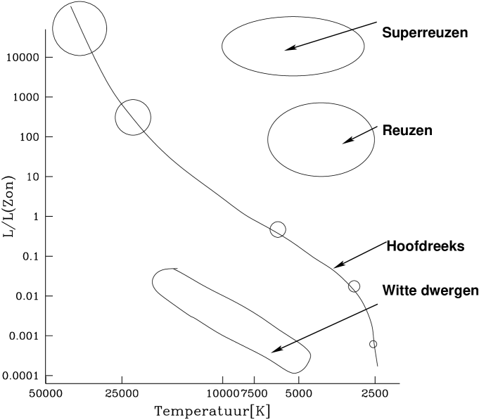
Figure 7: Grafiek van de helderheid van een ster (de ’magnitude’) versus de temperatuur van de ster (de ’kleur’): dit type figuur heet een Hertzsprung-Russell (of HR) diagram, of ook wel een kleur-magnitude diagram. Astronomen gebruiken 2 criteria om sterren in deze figuur te classificeren. Het eerste criterium gebruikt het spectrum van de ster, de kleur van het licht dat de ster uitzendt. De kleur hangt af van de temperatuur van de ster. Zo ziet een hete ster (zoals Sirius) er blauw uit, terwijl een koele ster (zoals Betelgeuze) er rood uitziet. De zon is bijvoorbeeld geel. Het tweede criterium gebruikt de helderheid van de ster, dus eigenlijk de energie die per seconde door de ster wordt uitgezonden. Sterren liggen niet kris-kras verspreid in een HR diagram, maar ze liggen op bepaalde banden (reeksen). Elk van deze banden correspondeert met een zekere fase in het leven van de ster, i.e. een zekere manier waarop kernfusie plaatsvindt in het centrum van de ster.

The $(J-K)_{0}$ vs. $(H-K)_{0}$ colours of Mira stars are shown in Fig. 7. For stars with low mass-loss rate ($<10^{-7}$ M_⊙ yr^-1) $(J-K)_{0}$ ranges between 1.2 and 1.6 (Whitelock et al. 2000). Dust-enshrouded IRAS AGB stars with mass-loss rates of $10^{-6}-10^{-4}$ M_⊙ yr^-1 (Olivier et al. 2001) are much redder, $(J-K)_{0}$ ranging from 2 to 6.5 mag. The overall distribution appears to form a sequence of ever redder colours with increasing mass-loss rate, a trend that is well reproduced, e.g., by a model for an M10 type AGB star with increasing shell opacity (Groenewegen & de Jong 1993). Thus, a higher mass loss has the same effect on $(J-K)_{0}$ and $(H-K)_{0}$ colours as more interstellar absorption/reddening, making a distinction between intrinsic and interstellar reddening in these colours impossible.

In, both, the $(J-K)_{0}$ vs. $(K-[12])_{0}$ and the $(H-K)_{0}$ vs. $(K-[12])_{0}$ planes Mira stars are distributed along a broad sequence compared to that seen in the $(J-K)_{0}$ vs. $(H-K)_{0}$ plane, as shown in Figs. 8 and 9.

A comparison with the best fit to the colour-colour sequence of IRAS-selected oxygen-rich AGB stars (van Loon et al. 1998, 1997) shows that in the $(H-K)_{0}$ vs. $(K-[12])_{0}$ plane Mira stars lie below that curve, while in the $(J-K)_{0}$ vs. $(K-[12])_{0}$ plane there appears no such offset. The offset could be due to water absorption bands in the $H$ band (Frogel & Whitford 1987; Glass et al. 1995), that are found strong in large amplitude variable AGB stars, although we could not find any correlation between colour and variability index for the IRAS stars used by van Loon et al. (Fouque et al. 1992; Guglielmo et al. 1993). The offset might then indicate that for such cold stars the Carter (1990) transformations between the ESO photometry (Fouque et al. 1992; Guglielmo et al. 1993) and the SAAO system (van Loon et al. 1998, 1997) are not adequate.

Mira stars with $0.2<(H-K)_{0}<3$ mag fit

$$(K-[12])_{0}=4.26(\pm 0.04)+5.95(\pm 0.17){\rm~{}log}(H-K)_{0},$$

with an rms deviation of 0.5 mag. Although we use the SAAO system (Carter 1990), in Appendix A we show that this relation is also valid in the 2MASS photometric system.

4 Interstellar extinction and intrinsic colours of the SiO targets

Figure 10: Left panel: 2MASS $J-H$ versus $H-$K_S colours. Stars with upper magnitude limits are not shown. Dots and triangles represent objects with K_S smaller and larger than 6.0 mag, respectively. Filled and open symbols represent SiO detections and non-detections, respectively. The arrow shows the reddening vector for A${}_{\rm K_{\rm S}}$ $=1$ mag. Right panel: 2MASS K_S$-[15]$ versus $H-$K_S colours. Symbols are as in the left panel. The curve represents the best fit to the colours of known Mira stars (see Sect. 3).

Figure 11: Left panel: Dereddened 2MASS $(J-H)_{0}$ versus ($H-$K_S$)_{0}$ colours. Right panel: Dereddened 2MASS (K_S$-[15])_{0}$ versus ($H-$K_S$)_{0}$ colours. Symbols are as in Fig. 10. “Foreground objects” have been removed.

The observed colours of the SiO target stars are shown in Fig. 10. For a given K_S$-[15]$, the $H-$K_S colours of the SiO target stars are redder than those expected from the colour-colour relation of known Mira stars, and some stars show excess larger than $E(H-$K_S) $=1$ mag. This is due to interstellar extinction along the line of sight.

Since observations of Mira stars may suffer from several magnitudes of circumstellar reddening, it not possible to estimate the interstellar extinction toward the SiO target stars by simply assuming an intrinsic colour for a given star.

As seen from Figs. 7, 8 and 9, Mira stars follow near- and mid-infrared colour-colour relations. In the first figure, Fig. 7, the reddening vector is parallel to the distribution of observed stellar colours and to those of models of AGB stars of increasing shell opacity. In contrast, the reddening vectors in Figs. 8 and 9 have a slope smaller than that of the distribution of observed stellar points and in principle can permit a separation between interstellar and circumstellar extinction. However, the dispersion of the Mira stars around the colour-colour fiducial sequence is large (0.5 mag), due to the non-contemporaneity of the near- and mid-infrared data and because of the dependence of such relations on metallicity and stellar spectral type. The uncertainty of the interstellar extinction estimates by shifting a star along the reddening vector onto the $H-K_{\rm s},K_{\rm s}-[15]$ curve is larger than A${}_{\rm K_{\rm S}}$$=1$ mag for $K-[15]>3.5$ mag.

Therefore, to deredden our targets we prefer to use the “field” extinction values (reported in Table 3), i.e. we assume that a given SiO target star is located at the distance of the median extinction along the line of sight. Though the dispersion of individual field star extinctions along a given line of sight is considerable (from 0.1 to 0.8 $\sigma_{\rm A_{\rm K_{\rm S}}}$), the distribution is strongly peaked, especially in the Bulge region. This means also to assume that the SiO targets are located in the region with the highest stellar density along the line of sight. This assumption is justified by the fact that the lifetime of a star on the AGB evolutionary phase is very short ($\sim 5$% of the time spent on the helium core burning phase and from 0.1 to 2% of the time spent on the main sequence phase of such a star; Vassiliadis & Wood 1993) and we therefore expect most of the AGB stars to be located in those regions with higher stellar density.

The distribution of the SiO targets in the dereddened $(H-K_{\rm S})_{0},(K-[15])_{0}$ diagram (Fig. 11) approaches that of known Mira stars. This confirms that the “field” median extinction is a good approximation of the interstellar extinction for most of the SiO targets and that the SiO targets do mostly belong to the highest stellar density region, i.e. the inner Galaxy. There is still an asymmetry in the distribution of the SiO targets around the fiducial colour line of known Miras, which suggests that we could have underestimated the interstellar extinction for part of the sample. In regions of high extinction, due to their high near-infrared luminosity, Mira-like stars are detectable to larger distances than ordinary field stars. Deeper infrared observations are needed to obtain more accurate extinction estimates (Figer et al. 2004).

1 “Foreground objects”

Dereddening all observed points in the ($H-K_{\rm s})$ vs. $(J-H)$ diagram (cf. Fig. 7) to the A${}_{\rm K_{\rm S}}$$=0.0$ position, we can measure the total (circumstellar plus interstellar) extinction of each SiO target (Table 3). We assumed a stellar photospheric $(J-K_{\rm s})_{0}$ colour of 1.4 mag and a $H_{0}-K_{\rm S0}$ colour of 0.5 mag.

The difference of such total extinction estimates from 2MASS and DENIS $J,K_{\rm s}$ data gives an rms of $\Delta$A${}_{\rm K_{\rm S}}$ $=0.2$ mag, while the estimates from 2MASS $H-K_{\rm s}$ and $J-K_{\rm s}$ colours gives an rms difference of $\Delta$A_K $=0.13$ mag. For only 12 SiO targets we do not have any observed $H-K_{\rm s}$ or $J-K_{\rm s}$ values, and therefore total extinction values are not determined (Table 3).

The median interstellar extinction of the field stars surrounding a target star was compared with the individual total extinction of the target star. As expected, on average the target stars show larger total extinctions than their field stars. This is not the case, however, for a group of $\sim 50$ mostly very bright target stars (K_S $<6.0$), at various longitudes, marked with flag 1 in Table 3, which have total extinctions lower (a least 1$\sigma_{\rm A_{\rm K_{\rm S}}}$) than the “field” extinction and are therefore likely to be significantly less distant. Thereby the extinction was used to identify foreground objects. We dereddened the “foreground objects” by directly shifting them on the $H,K_{\rm s},[15]$ colour-colour sequence.

5 Intrinsic colours and mass-loss rates

The stellar mass-loss rate is best estimated from measurements of CO rotational lines. The CO emission arises in the circumstellar shell. However, because of confusion with interstellar CO emission it is difficult to obtain such measurements toward stars in the inner Galaxy (Winnberg et al. 1991). Although infrared emission also arises from the stellar photosphere, stellar outflows may be studied from the infrared emission of dust grains which form in the cool circumstellar envelopes. Relations between the infrared colours (e.g. $J-K$, $K-L$, $K-[12]$ or $K-[15]$) of O-rich AGB stars and their mass-loss rate have been established empirically (e.g. Whitelock et al. 1994; Olivier et al. 2001; Alard et al. 2001) and supported by theoretical models (e.g. Groenewegen & de Jong 1993; Ivezíc et al. 1999; Jeong et al. 2003; Ojha et al. 2003).

The empirical relation between the $(K-[15])_{0}$ colour and the mass loss rate, $\dot{M}$, is very useful to study stars detected in the 2MASS, DENIS, ISOGAL or MSX surveys toward the most obscured regions of the Galaxy.

The uncertainties arising from the variability of the stars and the temporal difference between the K_S and 15$\mu$m measurements, is somewhat alleviated by using an average of the 2MASS and DENIS K_S fluxes and of the ISOGAL and MSX 15$\mu$m measurements (Ojha et al. 2003). The remaining r.m.s. uncertainty of the mass-loss rate is thus a factor $\sim$2 for $\dot{M}>10^{-6}$ M_⊙ yr^-1.

Figure 12: Distribution of mass-loss rates derived from the $K-[15]$ vs. $\dot{M}$ relation Jeong et al. (2003). The continuous line shows the distribution for all SiO targets dereddened using Lutz’s extinction law (Curve 3), and the dotted line that of foreground stars. The dashed line is the distribution of all SiO targets using the mid-infrared extinction law of Mathis (Curve 1).

Following the prescription of Jeong et al. (2003) and Ojha et al. (2003) we obtained mass-loss rates for the SiO targets, the distribution of which is shown in Fig. 12. 90% of the sources have implied mass loss rates between $10^{-7}$ and $2\times 10^{-5}$ M_⊙ yr^-1, with a peak in the range $10^{-6}$ – $10^{-5}$ M_⊙ yr^-1, although the apparent distribution is widened by the uncertainty of the mass-loss–colour relation, by the photometric uncertainty and by the effects of variability. Note that the selection criterion on (K_S$-[15])_{0}$ for the ISOGAL sample completely eliminated sources with $\dot{M}>10^{-5}$, and that the elimination of OH/IR sources and the criteria on $A-D$ and $C-E$ colours for the MSX sample also considerably reduced the proportion of sources with large mass-loss rates (see ; , ). The same results are obtained considering the subsample of targets with the best extinction corrections, i.e. with $\sigma_{\rm A_{\rm K_{\rm s}}}<0.2$ mag. The distribution of the mass-loss rates of the SiO targets with detected SiO maser emission appears similar to that of the SiO targets non-detected (Chapter II).

Adopting Mathis’ mid-infrared extinction law rather than Luts’s one, the distribution of the mass-loss rates only slightly shift toward lower values (see Fig. 12).

6 Conclusion

We estimated the interstellar extinction toward each of our 441 SiO target stars. For all 2MASS stars within 2-4 radius field of each target we shifted the $(J-K_{\rm s})$ and $(H-K_{\rm s})$ colour versus $K_{\rm s}$ magnitude along the reddening vector onto the reference red giant branch. The use of both colour-magnitude planes enabled us to obtain a mean extinction for each field and new constraints on the index of the near-infrared extinction power law, $\alpha$. We found that a value of $\alpha=1.6$ is inconsistent with the colours of inner Galactic stars, and, taking 47 Tuc as a reference for the RGB, we determine $\alpha=1.9\pm 0.1$.

For K_S-band extinctions larger than 1.6 mag the 2MASS $(K_{\rm S},J-K_{\rm s})$ CMD yields too low extinction estimates, due to a selection effect from the $J$-band dropout of more distant sources. The 2MASS ($K_{\rm s},H-K_{\rm s}$) CMD suffers less from this bias.

We reviewed near- and mid-infrared dereddened colour-colour relations of Mira stars and use them to test the quality of the extinction corrections for each SiO target.

Under the assumption that SiO targets are spatially distributed similarly to surrounding field stars, we corrected the photometric measurements of the SiO targets adopting the median extinction of their surrounding field stars. Derredened colours of the SiO targets are not perfectly symmetrically distributed around the fiducial colour-colour line derived from known Mira stars, suggesting that for part of the SiO targets we may still be underestimating the interstellar extinction of up to about 15%. About 50 SiO targets lie significantly in the “foreground” of the mean stellar distribution.

Using the relation between mass-loss rate and (K_S$-15)_{0}$ colour given by Jeong et al. (2003), we estimated that most of the SiO targets have mass-loss rates in the range 10^-7 to 10^-5 M_⊙ yr^-1.

Appendix 3.A SAAO and 2MASS colours and magnitudes

Transformation equations between the colours and magnitudes measured in the SAAO Carter (1990) and 2MASS photometric systems have been derived by Carpenter (2001) using a list of mostly blue 94 photometric standards. Figure 12 in Carpenter (2001) shows that the differences between magnitudes and colours obtained with the two systems are smaller than 0.15 mag.

Considering that Mira stars have typically a pulsation amplitude in the near-infrared of 1-2 mag and that 2MASS data are from a single-epoch observation randomly taken with respect to the stellar phase, the system transformations have only a secondary effect in the total colour and magnitude uncertainty, when comparing data from 2MASS with data taken with the SAAO telescope.

Since Mira stars are cold objects, molecular absorption bands characterise their infrared spectra and we must exclude that a combination of molecular bands and filter transmissions could generate a different colour transformation for these special class of objects. To address that we looked for 2MASS counterparts of the 104 outer Bulge Mira stars monitored by Whitelock et al. (1994). As demonstrated in Chapter III, Mira stars are among the brightest objects detected in the $K_{\rm s}$ band and therefore the identification of their 2MASS counterparts is straightforward. A number of 101 2MASS counterparts were found within 60 (mostly within 10) from the IRAS position. We excluded three sources because they had not unique counterparts (IRAS 17287$-$1955, IRAS 17030$-$2801, IRAS 18264$-$2720).

The differences between the mean magnitudes obtained with SAAO observations (Whitelock et al. 1991) and the single-epoch 2MASS data have a dispersion of up to 0.8 mag.

Figure 13: Colour-colour plots of Mira stars. The dots indicate average colours of Mira stars obtained from SAAO observations (Whitelock et al. 1991). Crosses indicate colours from single-epoch 2MASS data for the same sample of Mira stars (Whitelock et al. 1991).

We obtain the following mean differences:

$${K_{\rm s}}_{(\rm 2MASS)}-K_{(\rm SAAO)}=-0.15\pm 0.06{\rm~{}mag};$$

$$(J-K_{\rm s})_{(\rm 2MASS)}-(J-K)_{(\rm SAAO)}=-0.14\pm 0.05{\rm~{}mag};$$

$$(H-K_{\rm s})_{(\rm 2MASS)}-(H-K)_{(\rm SAAO)}=-0.06\pm 0.03{\rm~{}mag}.$$

To verify whether the colour-colour relations found in Sect. 3, using data in the SAAO photometric system, hold also when using 2MASS photometry, in Fig. 13 we plot both SAAO data and 2MASS data for the same sample of Mira stars (Whitelock et al. 1991). No systematic trend is present.

Appendix 3.B IRAS and MSX filters

Most of the past work has been carried out using the IRAS photometry, and therefore the currently available colour-colour relations of Mira stars use mid-infrared data from the IRAS catalogue. A comparison of mid-infrared filters is therefore mandatory to translate old findings into new MSX and ISOGAL colours.

Figure 14: Colour-Colour diagrams of our SiO targets. The IRAS 12$\mu$m magnitude is defined as $[12]=-2.5\log F_{12}[{\rm Jy}]/28.3$. The continuous lines are our best fits.

Figure 14 shows the difference between MSX magnitudes and IRAS 12 $\mu$m magnitude for the SiO targets. Note that the $D$ filter excludes the silicate feature around 9.7 $\mu$m, while $A$ and $C$ filters include part of it (see Fig. 1). Therefore the ($D-[12])$ colour shows a dependence on the ($C-D$) colour, which increases when the silicate feature at 9.7 $\mu$m starts to be self-absorbed. The ($A-[12]$) and ($C-[12]$) colours do not show any trend with the ($C-D$) colour. Due to both uncertainties of photometric measurements and source variability the scatter is large, however we derived relations between the $A$, $C$, and $D$ and the [12] magnitudes, as follow:
$A-[12]=1.15\pm 0.03$ mag
$C-[12]=0.05\pm 0.03$ mag
$D-[12]=0.08(\pm 0.18)-1.13(\pm 0.05)(C-D)$ mag.

Chapter 4 86 GHz SiO maser survey of late-type stars in the Inner Galaxy IV. Bolometric magnitudes

Bolometric magnitudes

M. Messineo, H. J. Habing, K. M. Menten, A. Omont, L. O. Sjouwerman

Appendix 4.A Introduction

The early 1960’s observations of non-circular gas motions in the inner Galaxy produced evidence for the existence of a Galactic bar (de Vaucouleurs 1964). Its existence is also supported by an apparent asymmetry of the integrated light as seen in COBE maps (Blitz & Spergel 1991) and of the stellar counts (Nakada et al. 1991). Thus, stellar kinematic studies provided less stringent constraints, due to the small number of measured stellar radial velocities. OH and SiO maser emission lines from the envelopes of evolved late-type stars can measure stellar line-of-sight velocities with an accuracy of a few km s^-1 throughout the Galaxy. Maser emission thereby provides a ready means to measure line-of-sight velocities in the Galactic plane even where the optical interstellar extinction is high.

Lewis (1989) analysed the colours and maser emission of IRAS sources, suggesting a chronological sequence of increasing mass-loss from SiO, to H₂O and OH maser emission. This sequence links AGB stars through the Mira and OH/IR stages with Planetary Nebulae. The presence of particular maser lines apparently depends on the envelope’s mid-infrared opacity: a higher mass-loss rate makes a more opaque dust shell, which better shields molecules against photodissociation. However, parameters other than mass-loss, such as initial stellar masses and chemical abundances, probably also play an important role (Habing 1996).

A number of maser surveys have been carried out to measure stellar line-of-sight velocities toward the inner Galaxy, between 30 and $-30$ in longitude, (e.g. Baud et al. 1979; Lindqvist et al. 1992; Blommaert et al. 1994; Sevenster et al. 2001, 1997a, 1997b; Sjouwerman et al. 1998; Izumiura et al. 1999; Deguchi et al. 2000b, a). These surveys mostly detected visually obscured OH/IR stars, i.e., AGB stars with 1612 MHz OH maser emission and high mass-loss rates.

Our survey of 86 GHz SiO maser emission towards infrared-selected Mira-like stars in the inner Galaxy, mostly at $b<0.5$, (Messineo et al. 2002, hereafter Chapter II) led to the determination of 255 new line-of-sight velocities. The sample of targets (hereafter “SiO targets”) was selected to be complementary to previous OH/IR surveys, so the sources with the reddest mid- and near-infrared colours were excluded.

In studying Galactic structure and kinematics it is important to combine the kinematic information and the stellar properties, such as luminosities, to explore any differences in the velocity fields of different tracers. In particular, it must be clarified whether OH/IR and SiO masing stars trace the same dynamic population, so that they can simply be combined to study the kinematics of the inner Galaxy.

The infrared photometry of our 441 SiO targets, derived from the large surveys DENIS (Epchtein et al. 1994), 2MASS (Cutri et al. 2003), ISOGAL (Omont et al. 2003; Schuller et al. 2003) and MSX (Egan et al. 1999; Price et al. 2001), was given by Messineo et al. (2004b, hereafter Chapter III). Corrections for interstellar extinction were discussed by Messineo et al. (2004a, hereafter Chapter IV). The present paper derives the bolometric magnitude of each target star, which we then compare with those of a sample of OH/IR stars.

Since most of the SiO targets are variable stars (Chapter III), their characterisation would require long-term, multi-frequency flux monitoring programs, which are not available yet. A first, although necessarily approximate discussion of their luminosities is possible even with single epoch observations, making use of the most recent infrared surveys.

The individual source numbers (e.g #99) are taken from Table 2 (86 GHz SiO maser detections) and Table 3 (non-detections) of Chapter II.

Appendix 4.B Apparent bolometric magnitudes

The photometric measurements of each SiO target (Chapter IV) were corrected for interstellar extinction using the mean K_S–band extinction found from the surrounding field stars. For the wavelength-dependence of the extinction, we assume a power law $A_{\lambda}/A_{K}=(\lambda/2.12\mu m)^{-1.9}$, so that for the individual bands we find effective band extinctions (A_I, A_J, A_H) = (6.78, 2.86, 1.66) A${}_{\rm K_{\rm S}}$. For the mid-infrared range we use the extinction law of Lutz (the extinction ratios are given in Table 2 of Chapter IV, ).

The bolometric stellar magnitudes, $m_{\mathrm{bol}}$, were computed by integrating over frequency $\nu$ using linear interpolations between the dereddened flux densities, $F_{\nu}(\nu)$. At the low frequency end we extrapolated to $F_{\nu=0}=0$, and at the upper end we extrapolated the two highest frequency data–points, provided the flux decreases, to zero intensity. Loup et al. (2004) presented a comparison of different methods commonly used to compute bolometric magnitudes. Using model spectra of O-rich AGB stars (from Groenewegen & de Jong 1993), they showed that the integration method we adopt yields bolometric magnitudes which should on average be accurate within 0.3 mag. Since the DENIS $I,J,$K_S as well as the 2MASS $J,H,$K_S observations were each taken simultaneously, but both sets at different times, we computed the bolometric magnitudes separately using either the DENIS or 2MASS data. The SiO targets are mostly variable stars (Chapter III), so a comparison of both datasets yields some information on their average variability.

For all but two of the SiO target stars the low-frequency extrapolation is insignificant since it contains a negligible fraction of the total flux. Only for sources #76 and #347 the low-frequency extrapolation contributes more than 20% to the total integrated flux.

Given that usually (K_S$-[15])_{0}<5$ mag, the main uncertainty in computing the bolometric magnitudes of the SiO target stars arises from the extrapolation at high frequencies. For 20 SiO targets a linear extrapolation was not possible because the flux density rises at high frequencies. For another 100 targets the blue extrapolation using 2MASS data or DENIS data contributes more than 20% to the bolometric flux.

For about half of our SiO stars (233 stars) we could compute bolometric magnitudes through a direct integration using either the DENIS or 2MASS data, with the flux in the extrapolated regions contributing less than 20% to the total. Unless otherwise stated, we adopt the average of these two integrations to attenuate the effect of variability.

For the other half of our sample, a bolometric magnitude could be integrated from only one dataset, since either the other data set is incomplete or the blue extrapolation is too uncertain in that the extrapolated spectral region contributes more than 20% to the total flux. For this half of the sample, when both the DENIS and 2MASS K_S measurements were available, we estimate bolometric magnitudes using the bolometric corrections described in Appendix A and the average of the two K_S–band flux densities. The average flux densities at 15 $\mu$m, when both ISOGAL and MSX 15$\mu$m measurement were available, was used.

The apparent bolometric magnitudes are plotted against the (K_S$-[15])_{0}$ colour in Fig. 1. There is an misleading correlation because the range in $[15]_{0}$ is small compared with the range in $K_{\rm s0}$, and $m_{\mathrm{bol}}$ is dominated by the near-infrared flux.

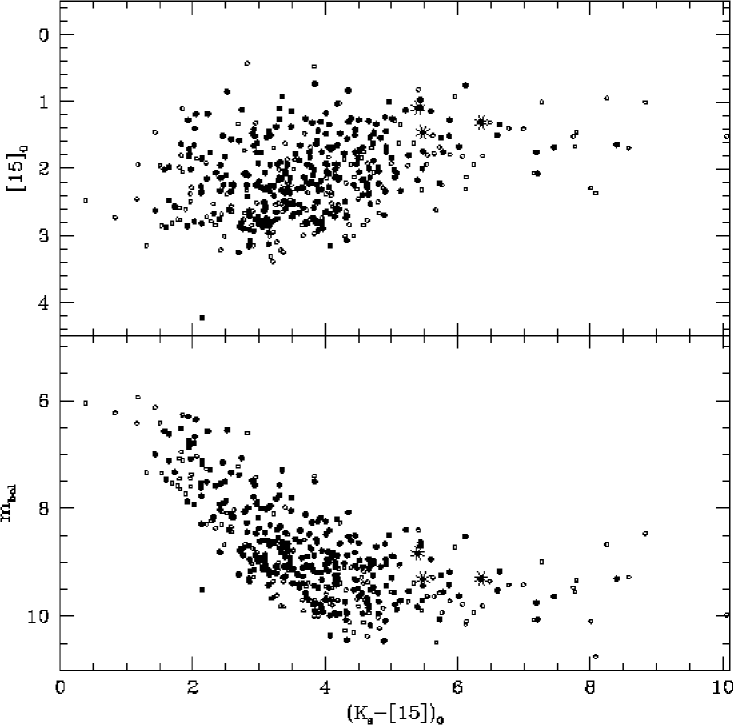
Figure 1: Lower panel: Apparent bolometric magnitudes, $m_{\mathrm{bol}}$, versus (K_S$-[15])_{0}$. Filled circles indicate objects with detected SiO maser emission, and open circles objects with no SiO detection. The four starred symbols show stars with observed OH emission (Chapter III). When both DENIS and 2MASS K_S measurements are available, or when both ISOGAL and MSX 15$\mu$m measurement are available, the average flux density is adopted. Upper panel: Apparent $[15]_{0}$ magnitudes versus the (K_S$-[15])_{0}$ colour. Symbols are as in the lower panel.

There is a tail of stars at faint apparent bolometric magnitudes with a wider colour spread and redder (K_S$-[15])_{0}$ colours (Fig. 1) (which is the consequence of selection of MSX sources, Chapter III, ). These redder colours are indicative of higher mass-loss rates.

1 Variability

Bolometric magnitudes of known Mira variables are found to vary up to 2 mag from minimum to maximum light (e.g. Whitelock et al. 2000, 1991).

Since we are using single epoch observations taken at random phase, the obtained bolometric magnitudes are also at a random phase.

Figure 2 shows that there is an rms scatter of $\sim 0.35$ mag between $m_{\mathrm{bol}}^{2MASS}$ and $m_{\mathrm{bol}}^{DENIS}$, which is mainly due to variability (Chapter III). There is a tight correlation between $m_{\mathrm{bol}}$ and K_S since both quantities are related by the bolometric correction $BC_{K_{\rm s}}$ (Appendix A). If we assume that all stars are sinusoidally variable with maximum-to-minimum amplitudes $A_{i}$, and that 2MASS and DENIS measurements are unrelated in time, then the rms of the amplitude distribution is equal to the rms of the differences between two measurements at random phase, i.e. 0.35 mag.

The observed scatter is only a lower limit to the stellar flux variability, because it only accounts for the near-infrared variation. However, since the dominant part of the stellar energy distribution of a Mira star is at near-infrared frequencies and since its pulsation amplitude decreases at lower frequencies, this variation is nearly that of the bolometric flux.

Figure 2: Left panel: Apparent bolometric magnitudes derived using 2MASS data versus apparent bolometric magnitudes using DENIS data. Right panel: Differences in $m_{\mathrm{bol}}$ versus the corresponding differences between DENIS-K_S and 2MASS-K_S.

Appendix 4.C SiO targets with $|l|<5^{\circ}$

1 Luminosities

We derive the “absolute” bolometric magnitudes, $M_{\mathrm{bol}}$, of 252 sources within the central 5 of the Galactic Centre adopting a distance of 8 kpc. Their “absolute” bolometric magnitudes, as shown in Fig. 3, ranges from $-4$ to $-8$ mag, with a peak around $-5.0$ mag. Our SiO targets appear to have mostly luminosities above that of the tip of the red giant branch at $M_{\mathrm{bol}}\sim-3.6$ (Ferraro et al. 2000), where the helium flash stops the ascent of the star on the red giant branch. This is typical for long period variable (LPV) stars in old metal-rich globular clusters.

Only two SiO targets (#77 and #347) have $M_{\mathrm{bol}}$ fainter than $-4.0$ mag; those stars could be in the early AGB phase or at a larger distance, or could have lower initial masses than the bulk of the SiO targets.

Figure 3: Distribution of absolute bolometric magnitudes for an adopted distance of 8 kpc. SiO targets identified as possible foreground objects on the basis of their extinction (Chapter IV) are omitted from the plot. Upper panel: The dotted line shows the distribution of all SiO targets with $|l|<5^{\circ}$. The continuous line shows the distribution of SiO stars with (A${}_{\rm K_{\rm S}}$$>2.0$ mag); most of them belong to the Nuclear Disk (see Sect. 4.F). Lower panel: For comparison the distribution of absolute magnitudes of a sample of OH/IR stars within 1 from the Galactic centre (Ortiz et al. 2002) is shown.

Another 33 (11%) of all SiO targets within 5 degrees from the Galactic Centre have $M_{\mathrm{bol}}<-6.5$ mag, and even brighter than $-7.2$ mag, which is the classical AGB limit (Iben & Renzini 1983). The maximum average luminosity observed for Galactic Mira stars corresponds to $M_{\mathrm{bol}}$$=-5.5$ mag (Whitelock et al. 1991; Glass et al. 1995; Olivier et al. 2001). Since the K_S–band luminosity of a Mira star varies by up to about 2 magnitudes, for a single epoch measurement at random phase, we expect a distribution extending to $M_{\mathrm{bol}}=-6.5$ mag. The 33 targets brighter than this limit, could be either foreground stars, massive, young AGB stars, or evolved massive stars (red supergiants) (Nagata et al. 1993; Schuller 2002).

Near-infrared spectroscopy could reveal their true nature (e.g. Schultheis et al. 2003). By combining extinction information and luminosity Messineo et al. found that 20 of the 33 bright sources are likely to be foreground stars (Chapter IV). Their total extinction (interstellar plus circumstellar), which was calculated by assuming a photospheric colour for the central star, appears to be lower than the average interstellar extinction of stars in their respective surrounding fields.

We find five sources (#31, #75, #92, #128, #294) with $M_{\mathrm{bol}}<-7.2$ mag that cannot be explained as foreground on the basis of their extinction. One of them (#92) is classified as a possible red supergiant stars by Nagata et al. (1993). The bolometric magnitude given by Nagata et al. is in good agreement with our measurement. It is not unlikely that some of our other bright sources are also red supergiants.

2 Initial masses and ages

Estimates of the initial mass of pulsating AGB stars is problematic due to uncertainties in the pulsation mode, effective temperature (i.e., stellar radii), and of the mass-loss history (e.g. Vassiliadis & Wood 1993; Marigo et al. 1996). A degeneracy between age and metallicity further complicates the analysis of the distribution of stellar colours and luminosities (e.g. Frogel & Whitford 1987; Whitelock et al. 1991; van Loon et al. 2003).

The maximum luminosity reached at the end of the AGB phase strongly depends on the metallicity and initial mass of the star: a lower metallicity leads to a higher luminosity for a given initial mass.

Assuming solar metallicity and using the relation from Marigo et al. (1996) between the initial mass and maximum luminosity reached before the onset of the superwind (Vassiliadis & Wood 1993; Renzini & Voli 1981), we derive a distribution of initial masses for our SiO targets that ranges from 1.0 to 4.0 M_⊙. This range is perhaps wider than the real due to the variability and our use of single epoch observations. For a solar metallicity, the majority of the SiO targets ($M_{\mathrm{bol}}=-4.5$ to $-5.5$) has ages ranging from 0.8 to 5 Gyr (Girardi et al. 2000). However, these are lower limits since stars with higher than the assumed solar metallicity would stay longer on the main sequence and would therefore be older when they reach the AGB.

A reliable empirical calibration of mass and age is possible only for Mira stars in globular clusters. Bulge Mira stars are more massive and/or metal rich than Mira stars in Galactic globular clusters (e.g. Whitelock et al. 1991), as follows from their longer pulsation period (up to 800 days vs. 200-300 days in globular clusters) and higher luminosity. The most luminous AGB star in globular clusters has $M_{\mathrm{bol}}=-4.8$ mag (Guarnieri et al. 1997), while in the bulge they can reach $-5.5$ mag (Whitelock et al. 1991; Glass et al. 1995).

The presence of an intermediate age population ($2.2M_{\odot}<$ initial mass $<8.0$$M_{\odot}$) in the inner Galaxy was suggested by, e.g., Cole & Weinberg (2002); van Loon et al. (2003). However, most of these studies are based on photometric observations of only giant stars. Because of differential reddening and the degeneracy between metallicity and age those studies could not securely confirm the presence of such a young population.

To infer the age of a stellar population it is crucial to detect the main-sequence turn-off. Using deep near-infrared photometry Zoccali et al. (2003) studied the stellar population of a bulge field at latitude $b=6$, from main–sequence stars to the AGB tip. They estimated an age of 10 Gyr for the field population and did not observe any other turn–off that could suggest the existence of an intermediate age population. Their number of luminous AGB stars agrees with that predicted for a population of that age. However, Zoccali’s field is at $b=6$  and it may not be representative of the in–plane population of the inner Galaxy.

Feltzing & Gilmore (2000) studied stars in the Baade’s window field using visual HST data and also concluded that bulge stars are generally old, although the existence of a young and metal–rich population cannot be ruled out.

Evidence for a younger component comes from the distribution of OH/IR stars, in the central bulge that have a vertical scale height $<100$ pc (Sevenster 1999b). They could belong to a distinct in–plane component. Furthermore, low latitude OH/IR stars stars and SiO targets do not trace the axisymmetric and old (8-10 Gyr) bulge population studied by Ng & Bertelli (1996), but the longitude–velocity diagram of maser stars shows evidence for a Galactic bar (Sevenster 1999b; Messineo et al. 2002). The masing population could be related to a more recent star formation event, e.g., triggered by the formation of the Galactic bar (e.g. Sevenster 1999b; Cole & Weinberg 2002; Sjouwerman et al. 1999).

New near–infrared photometric observations down to the main-sequence turn–off for inner Galactic fields at low latitude are important for improving our understanding of Galactic stellar population history, and can verify the possible existence of an intermediate age population.

Near–infrared spectroscopy would yield estimates of the metallicity of masing stars. The SiO targets, being bright at near–infrared wavelengths, are ideal targets for such a spectroscopic program.

3 Red Supergiant stars ?

Red supergiant stars are massive stars ($>9$ M_⊙), which are burning helium (or carbon) in non-degenerate cores. They are often located in OB associations. The luminosity distribution of the SiO targets within 5 from the Galactic Centre, shown in Fig. 3, suggests that a few red supergiant stars are also included, as supported by other indications described below.

IRAS counterparts of our SiO targets are mostly located in region IIIa of the IRAS two–colour diagram (Chapter III). Previous studies of IRAS sources have shown that most of the sources in region IIIa are O–rich AGB stars, but 26% may be red supergiant stars (Josselin et al. 1996; Winfrey et al. 1994).

Weak SiO maser emission is found in semiregular AGB and red supergiant stars (Alcolea et al. 1990), but red supergiants with large amplitudes are strong SiO emitters and their SiO maser intensity is comparable to that of Mira stars (Alcolea et al. 1990). The central star has an extended shell, generated by the strong pulsations as in LPVs, where the SiO maser activity takes place.

The line profile of the SiO masers normally has several components a few km s^-1 wide over a range from 10 km s^-1 (giant) to 20-40 km s^-1 (supergiant) (Alcolea et al. 1999; Le Bertre & Nyman 1990). Our entire sample has an average SiO maser line width of 4.6 km s^-1 with a scatter of 2.3 km s^-1. There are 12 sources with line width $>9$ km s^-1: #31, #71, #87, #113, #117, #129, #135, #173, #190, #203, #223, #232. These spectra look similar to the broad and multiple peaked spectra typical of red supergiants (Haikala 1990; Cho et al. 1998). Seven of those 12 are located within 5 of the Galactic centre, and 4 (#31, #87, #113, #129) are also very luminous ($M_{\rm bol}<-6.5$ mag). The velocity–longitude distribution of bright ($M_{\rm bol}<-6.5$ mag) stars detected in our SiO maser survey appears distinct from that of the nuclear disk component or from bulge stars. The linear dependence of $v$ and $l$ suggests (see Sect. 4.G) that it is probably a Galactic disk component.

Appendix 4.D Comparison with OH/IR stars

For a comparison with our SiO targets, we also consider a sample of OH/IR stars (AGB stars with 1612 MHz OH maser emission) within 1 from the Galactic Centre (from Table 3 of Ortiz et al. 2002), a region fully mapped at 1612 MHz (Lindqvist et al. 1992; Sjouwerman et al. 1998; Sevenster et al. 1997a). Ortiz et al. found ISOGAL counterparts for all OH sources in ISOGAL fields, counterparts which are typically bright at 15 $\mu$m and have very red (K_S$-[15])_{0}$ colours (reaching 12 mag; see upper panel of Fig. 4), which is indicative of high mass loss rates.

Figure 4: Lower panel: “Absolute” bolometric magnitudes, $M_{bol}$, versus dereddened (K_S$-[15])_{0}$, adopting a distance of 8 kpc. When both DENIS and 2MASS K_S measurements, or both ISOGAL and MSX 15$\mu$m measurements are available, the average flux density is adopted. Circles show SiO targets from the ISOGAL fields of Ortiz et al. (2002), they cover about $\sim 0.84$. Filled and open symbols indicate SiO maser detections and non–detections, respectively. For comparison, crosses show OH/IR stars within 1 from the Galactic Centre with a known period and ISOGAL counterpart (Ortiz et al. 2002). The line at $M_{\mathrm{bol}}=-3.6$ indicates the location of the tip of the red giant branch and the line at $M_{\mathrm{bol}}=-7.2$ the AGB limit. Upper panel: “Absolute” $[15]_{0}$ magnitudes, $M_{[15]}$, versus dereddened (K_S$-[15])_{0}$. Symbols are as in the lower panel.

To directly compare luminosities of OH/IR stars with those of SiO targets, bolometric magnitudes must be calculated in the same way. We therefore calculated the interstellar extinction A${}_{\rm K_{\rm S}}$ toward each OH/IR star using 2MASS stars within 2 from the position of the OH/IR star, following the procedure described in Chapter IV. Extinctions, A${}_{\rm K_{\rm S}}$, are found systematically larger (by up to 0.6 mag) than those adopted by Ortiz et al. (2002). This is due to our use of the ($H$, K_S) data, which are less sensitive to extinction and therefore less affected by a low–extinction bias than ($J$, $H$) or ($J$, K_S) data used by Ortiz et al. (2002). We adopted the near–infrared mean flux densities of the OH/IR stars given by Wood et al. (1998). When using Mathis’ extinction law (for comparison with Ortiz et al. 2002) we obtained bolometric magnitudes consistent with those of Ortiz et al. (2002): since the spectral energy distribution of an OH/IR star peaks long-ward of 3$\mu$m (due to the presence of a thick circumstellar envelope), its bolometric magnitude is less sensitive to near–infrared interstellar extinction corrections than for SiO targets. However, when we adopt the mid–infrared extinction law suggested by Lutz et al. (as for the SiO targets, Chapter IV, ) we obtain bolometric magnitudes for the OH/IR stars brighter by up to 0.6 mag. Whenever a bolometric magnitude determination via direct integration (Sect. 4.B) was not possible, it was estimated using the bolometric correction described in the Appendix.

Figure 3 shows a comparison between the bolometric magnitude of our SiO targets (Sect. 4.B) with that of the OH/IR stars.

The peak of the OH/IR magnitude distribution is at $\sim-5.1$ mag, and translates to an initial stellar mass of about 1.8 $M_{\odot}$ and an age of about 2 Gyr, using the models of Girardi et al. (2000) with solar metallicity. The peak for OH/IR stars appears consistent with the median of the bolometric magnitudes of SiO targets in the central 5, although the distribution of the latter is broadened by variability and the use of single epoch observations.

For the 96 SiO targets (58 detections) from the same ISOGAL fields as the OH/IR stars of Ortiz et al. (2002), Fig. 4 shows the absolute bolometric magnitude of both OH/IR and SiO stars plotted against their (K_S$-[15])_{0}$ colour. Distributions appear to differ in that SiO targets have bluer colours (due to our selection, Chapter III, ). This indicates that OH/IR stars have thicker envelopes due to higher mass–loss rates.

Note that here we are comparing only our SiO targets with known OH/IR stars. We imposed colour constraints for our target selection and we tried to be complementary to previous OH/IR studies by discarding the reddest mid- and near–infrared colour sources. It is quite well possible that there are SiO masing stars with colours much redder than what we considered, though according to Nyman et al. (1993) there should be a cut–off in the 86 GHz SiO maser intensity for very optically thick circumstellar envelopes.

In contrast to SiO targets, there are no OH/IR stars brighter than $M_{\rm bol}=-6.5$ (for a distance of 8 kpc) in our sample. The luminous SiO targets tend to be bluer than fainter ones, suggesting a thinner circumstellar envelope, which could also explain the lack of 1612 MHz OH maser line emission. Therefore, our sample includes luminous SiO masing AGB stars or red supergiants, with moderate mass–loss rates, not masing in OH. If the mass–loss rate increases with time (e.g. Lewis 1989) these objects could later also show 1612 MHz OH maser emission, which is more likely for thicker envelopes (Sevenster et al. 2001; Habing 1996).

In the chronological sequence of circumstellar masers presented by Lewis (1989), as first suggested by Bedijn (1987), circumstellar envelopes of AGB stars gradually evolve under slowly increasing rates of mass loss. Since the SiO masing shell is near the photosphere, the first maser emission to appear is that from SiO, while OH maser emission appears as the shell grows. The SiO maser emission is then the first to disappear when the mass loss declines.

The distributions of bolometric magnitudes of both SiO and OH/IR stars, as seen in Fig. 3, peak at about the same value, which suggests that both populations trace the same epoch of star formation, but SiO masing stars have less evolved circumstellar envelopes (see also Chapter III, ). This is supported also by the different distribution of SiO and OH/IR stars in the period–luminosity diagram (Sect. 4.E).

Appendix 4.E Period–Luminosity relation

Our SiO targets include 15 LPVs from the sample of Glass et al. (2001), see also Sect. 4.2 in Chapter II. Figure 5 plots their bolometric magnitudes against their periods, showing that they fall above the period–luminosity distribution of Mira stars in the Sgr–I field (Glass et al. 1995). However, in the Sgr–I field Mira stars with period longer than 450 days are rare. Our SiO stars may support a steepening of the period–luminosity relation for period longer than 450 days, as observed in the Magellanic Clouds (Hughes & Wood 1990).

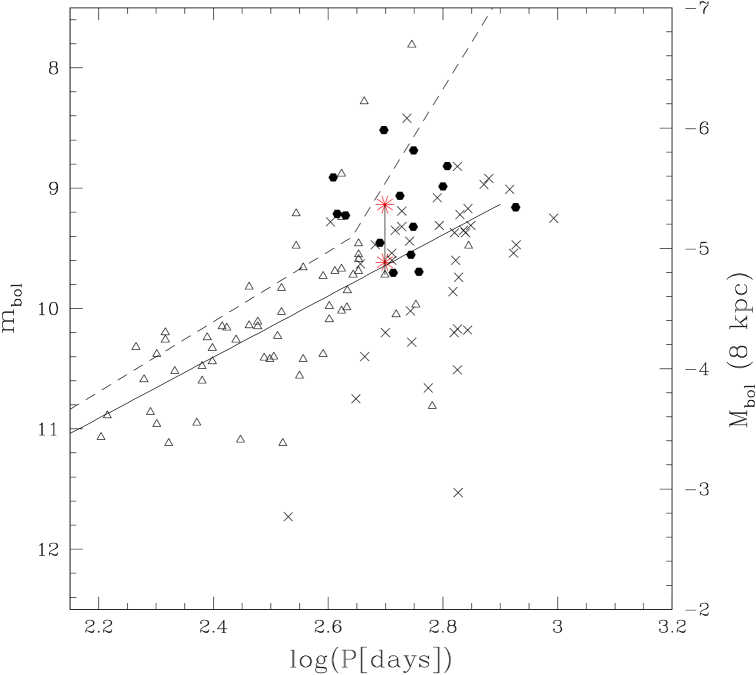
Figure 5: The period–luminosity relation of LPV stars. Dots represent 15 LPV stars in our SiO maser sample located within 24 from the Galactic Centre (Glass et al. 2001). They have a bright ISOGAL counterpart, but no known OH maser emission. Triangles show Mira stars located in the Sgr–I field (Glass et al. 1995), for which we plot the mean bolometric magnitudes. For #153, the only SiO target located in the Sgr–I field, we plot both magnitudes (stars) obtained using DENIS and 2MASS data, and connect them to the mean $m_{\mathrm{bol}}$ value found by Glass et al. (1995) with a vertical line. Crosses show OH/IR stars with ISOGAL counterpart (Ortiz et al. 2002). The continuous line represents the relationship found by Glass et al. (1995), while the dashed line is a fit for LMC Mira stars (Hughes & Wood 1990), assuming a distance modulus of 18.55 mag for the LMC and 14.5 mag for the Galactic Centre.

The standard deviation in the period–luminosity relation of Mira stars in Sgr–I is 0.36 mag (Glass et al. 1995), which partly arises from the spread in distance, and partly from the uncertainty in the apparent bolometric magnitude. A spread of $\pm 2$ kpc in distance at a distance of 8 kpc causes a spread in $M_{\mathrm{bol}}$ of $\pm 0.55$ mag. Bolometric magnitudes given by Glass et al. (1995) were obtained adopting the mean values of monitored infrared flux densities. The period–luminosity relation obtained using mean magnitudes of Mira stars in the Magellanic Clouds is less sensitive to distance uncertainties, resulting in a scatter of only 0.15 mag (Feast et al. 1989).

Our sample has one SiO star located in the Sgr–I field, #153. Its $m_{\mathrm{bol}}$ calculated using DENIS data is 9.62 mag, identical to the mean value obtained by Glass et al. (2001). When using 2MASS data we find $m_{\mathrm{bol}}=9.14$ mag. Considering the pulsation amplitude $\Delta K=1.38$ mag (Glass et al. 1995), both measurements are consistent.

The 15 LPV/SiO targets in the Galactic Centre from Glass et al. (2001) suffer from strong extinction (A${}_{\rm K_{\rm S}}$$>2$ mag) and using the kinematic information for the 11 which were detected in our SiO maser survey, we conclude that they are members of the central nuclear disk (see Sect. 4.F). They are therefore at about the distance of the Galactic centre. Assuming an isotropic distribution of stars in the nuclear disk, a range of longitudes of $\pm 1.5$ translates to a distance range of $\pm 200$ pc, and a corresponding distance modulus range of $\pm 0.05$ mag. Their dispersion on the period–luminosity plane is mostly due to the uncertainty in the bolometric magnitude ($\sim$0.35 mag, see Sect. 4.B) and in the extinction (Chapter IV).

Since we selected bright ISOGAL and MSX sources (Chapter II) and since mid–infrared flux density correlates with period (see the 12$\mu$m period–luminosity relation in Whitelock et al. 1991), it is not surprising that the LPVs we observed have periods above 400 days (Fig. 5). Imai et al. (2002) searched for SiO maser emission toward the entire sample of Mira stars near the Galactic centre detected in $K$–band by Glass et al. (2001) and confirmed the expected increase of the detection rate with increasing period. While for periods below 300 days the SiO maser detection rate is below 20%, above 400 days it rises to 60% . OH/IR stars also have typical periods above 400 days (Fig. 5). Thereby, SiO and OH maser emission mainly trace long period AGB variables.

Unlike Mira stars, OH/IR stars do not follow a period–luminosity relation in the Galactic Centre region (Ortiz et al. 2002, and references therein). Most of them for a given magnitude have a longer period than that predicted by the Mira period–luminosity relation, so OH/IR stars and SiO targets are differently distributed.

Pulsation models predict that due to a dramatic increase of the mass loss rate (superwind phase), a Mira star significantly stretches its pulsation period, while its luminosity remains almost constant (Vassiliadis & Wood 1993), and becomes an OH/IR star. OH/IR stars have then longer periods for a given luminosity than those found in Mira stars.

Appendix 4.F Stars in the the Nuclear Disk and a fourth dimension: extinction

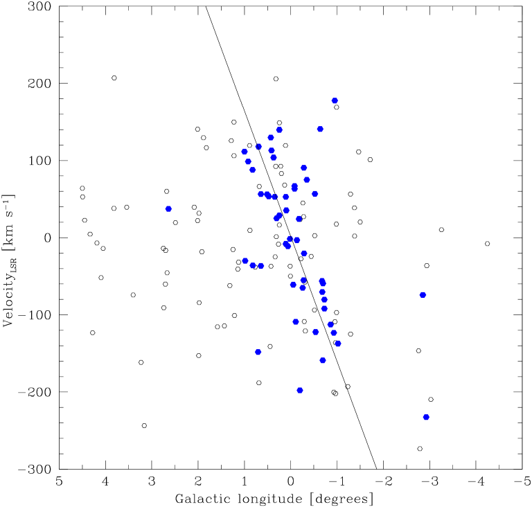
Figure 6: Stellar longitude–velocity diagram of our 86 GHz SiO masers. Filled circles indicate sources with interstellar extinction A${}_{\rm K_{\rm S}}$ above 2 mag. Most of these belong to the fast rotating nuclear disk. The continuous line indicates our best fit to the nuclear disk component.

The line of sight extinction is a useful fourth dimension along with position ($l,b$) and velocity to characterise various Galactic components.

Around zero longitude our stellar longitude–velocity ($l-v$) diagram reveals a stellar nuclear disk, which follows the high velocity gaseous nuclear disk (e.g. Burton & Liszt 1978; Binney et al. 1991).

There is a unique correspondence between interstellar extinction and velocity. When we select SiO targets at interstellar extinction A${}_{\rm K_{\rm S}}$$>$ 2 mag (Fig. 6), we find that most of these stars kinematically trace the nuclear disk. Their line–of–sight velocities range from $\sim+150$ to $\sim-200$ km s^-1, similar to the gaseous nuclear disk line–of–sight velocities (cf. the ¹³CO ($l-v$) diagram in Fig. 4 of Bally et al. 1988). Therefore, the extinction enables us to identify individual stars belonging to the nuclear disk.

The stellar nuclear disk rotates rapidly around the Galactic Centre: our best–fit yields a gradient of 162($\pm 40)$ km s^-1 per degree longitude. This slope is consistent with a value of $180(\pm 15)$ km s^-1 found for OH/IR stars with high circumstellar expansion velocity located within 1 of the the Galactic Centre (Lindqvist et al. 1992).

To investigate whether the 56 SiO targets with A${}_{\rm K_{\rm S}}$$>2$ mag also show distinct physical properties, their bolometric magnitude distribution is shown in Fig. 3. The distribution peaks at $-5.4$ mag, a peak slightly more luminous than the average luminosity of SiO targets within 5. However, their luminosity is consistent with those of variable AGB stars. There is only one SiO target with $M_{\rm bol}<-6.5$ mag, #99, which may be a young star. Its location ($l=0.8$; $v=-36.0$ km s^-1; $2\sigma$ away from our best fit) indicates that it is probably unrelated to the nuclear disk in origin and kinematics.

The 11 LPVs from Glass et al. (2001) that we detected at 86 GHz (see also Sect. 4.E) all belong to the nuclear disk population, as their positions ($|l|<1.5,|b|<0.5$), their interstellar extinctions (A${}_{\rm K_{\rm S}}$$>2.0$ mag) and their line–of–sight velocities confirm.

Appendix 4.G Bolometric magnitudes and the $l-v$ diagram

Different Galactic components give a different signature in the $(l-v)$ diagram. However, a stellar $(l-v)$ diagram alone is not sufficient to locate individual stellar components, mainly due to the velocity dispersion of the stars, that smooths various features. The inclusion of additional distance information will notably improve the understanding of the $(l-v)$ diagram. The stellar bolometric magnitude may serve as a first approximation of distance.

In section 4.C, we have already noticed the presence of a group of stars brighter than the typical luminosity of a Mira star at its maximum ($M_{\rm bol}=-6.5$ mag) when we assume a distance of 8 kpc. In Figure 7 we illustrate the $l-v$ diagram of SiO targets with $M_{\rm bol}$ fainter and brighter than $-6.5$ mag. The bright sample appears to be distributed differently from the faint sample, since it has a low velocity dispersion ($\sim 30$ km s^-1), independently of longitude. The stars that were classified as foreground stars on the basis of extinction consideration (crosses in Fig. 7; see also Chapter IV, ), almost all belong to the bright group. This indicates that the bright stars are closer on average to the Sun than fainter ones and that their luminosities are overestimated by assuming the distance of the Galactic centre. But then how nearby are those stars? Do they trace a specific Galactic component?

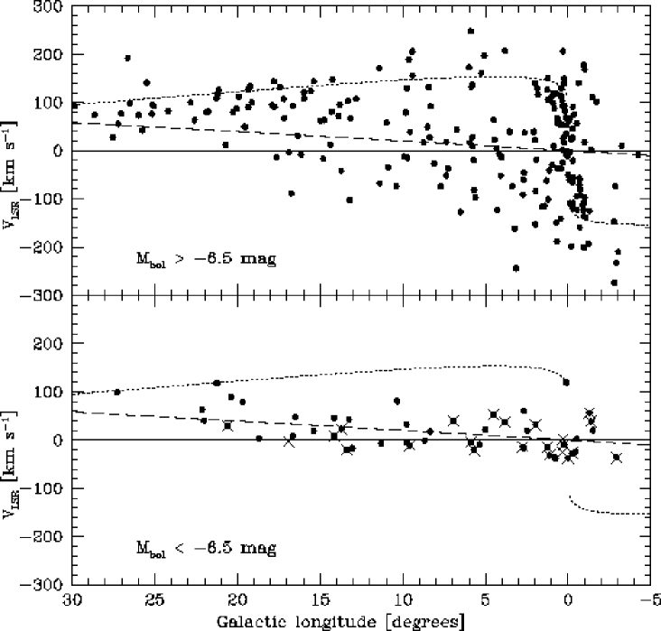
Figure 7: Longitude–velocity diagram of SiO targets. Upper panel: SiO targets with $M_{\rm bol}>-6.5$ mag (assuming a distance modulus for the Galactic centre of 14.5 mag). The dotted line shows the curve defined by the line-of-sight velocities of tangent points to circular orbits, as predicted by Eq. 5.1. The dashed line indicates a circular orbit at a galactocentric distance of 5 kpc. Bottom panel: Dots indicate SiO targets with $M_{\rm bol}<-6.5$ mag. Crosses indicate SiO targets classified as foreground on the basis of extinction (Chapter IV).

An estimate of their distance can be inferred by assuming circular orbits. However, this assumption clearly does not hold for the central kiloparsecs, due to both the presence of a bar and the fact that bulge stars might have a velocity dispersion larger than the rotation velocity. Hence, we calculated Galactocentric distances, under the assumption of circular orbits, for SiO targets at longitudes $>10$. We adopted the relation between the longitude, radial velocity and distance (Burton 1988):

$$v=R_{\odot}[\frac{V(R)}{R}-\frac{V(R_{\odot})}{R_{\odot}}]{\rm sin}(l),$$ (1)

where $V(R)$ is the circular rotation velocity at Galactocentric distance $R$, the Galactocentric distance of the Sun is taken to be $R_{\odot}=8.0$ kpc, and the circular velocity of the Sun $V(R_{\odot})=200$ km s^-1. Adopting $V(R)=V(R_{\odot})(R/R_{\odot})^{0.1}$ km s^-1 (Binney et al. 1991), and inverting equation (1), it follows that:

$$R=\frac{8.0}{(1+\frac{v}{(200\times{\rm sin}(l)})^{1.11}}({\rm in~{}kpc}),$$ (2)

Figure 8: Left side:The continuous histogram shows the distribution of Galactocentric distances inferred for SiO targets at longitudes $l>10$ using interstellar extinction estimates towards the line of sight of each SiO target and a model of Galactic dust distribution (Drimmel et al. 2003). The dotted histogram shows the distribution of Galactocentric distances inferred for SiO targets at longitudes $l>10$ assuming circular orbits. Right side: Distance estimates from interstellar extinction versus kinematic distances.

Bright sources are found to have an almost homogeneous distribution in Galactocentric distance, from 0 to 15 kpc. Fainter stars (Fig. 8) peak at about 3 kpc from the Galactic centre, i.e. at about the corotation radius of $\sim 3.4$ kpc (e.g. Englmaier & Gerhard 1999).

Since interstellar extinction increases with distance, another independent way to estimate distances is to use a model of dust distribution in the inner Galaxy. Using the implementation of Drimmel et al. (2003) based on COBE/DIRBE data, we calculated for each line of sight toward a SiO target the interstellar extinction as a function of distance. By interpolating the models at the values of derived interstellar extinction (Chapter IV), we have estimated distances to each SiO target.

The model of Drimmel et al. does not include the nuclear disk molecular complex and therefore it fails in reproducing the distance of nuclear disk stars. It predicts that all SiO targets are within a Galactocentric distance of 5 kpc and confirms a peak around corotation.

We used two independent methods to estimate distances, one based on kinematics and another based on extinction. Although the uncertainty are large (see right panel of Fig. 8), from both methods we find that most of SiO targets have a Galactocentric distance within 5 kpc, with a peak around corotation. The bright stars, however, do not seem confined at a specific Galactocentric distance.

It is difficult to argue about the nature of each single SiO target. The difference in distance modulus of a star at the Galactic centre and at a Galactocentric distance of 5 kpc is 2.1 mag, thus we might have overestimated the luminosity of the SiO target stars. The true luminosity of the “bright” stars could be below the AGB limit ($M_{\rm bol}<-7.2$ mag) and therefore they could be all AGB stars, rather than red supergiants. However, the luminosity range of these two classes of stars overlaps, and some of them could still be red supergiants as the SiO maser line widths and the low velocity dispersion suggest. Near–infrared spectroscopy is needed to distinguish between AGB and red supergiants. Furthermore, a near-infrared monitoring program would provide pulsation periods and therefore another independent estimate of the distance of each SiO target.

We are currently working on a kinematic study of the SiO targets based on a more realistic Galactic gravitational potential, which will be presented in a forthcoming paper.

Appendix 4.H Conclusion

Bolometric magnitudes for SiO target stars were computed from available flux density measurements. Adopting a distance of 8 kpc for all stars within 5 from the Galactic Centre we find a peak in the luminosity distribution at M${}_{\mathrm{bol}}=-5.1$ mag, which coincides with the peak shown by OH/IR stars in the Galactic Centre (e.g. Ortiz et al. 2002). Assuming a solar metallicity this peak magnitude corresponds to stars with an initial mass of 1.8 M_⊙ and an age of about 2 Gyr.

Our sample includes 15 LPVs from the sample of Glass et al. (2001). We found that these fall above the period–luminosity relation found by Glass et al. (1995), thus differing from OH/IR stars. This supports a chronological sequence for circumstellar masers proposed by Lewis (1989). We also find evidence for a steepening of the bulge period–luminosity relation for periods larger than 450 days, as found for Magellanic Cloud LPVs.

In contrast to OH/IR stars (Ortiz et al. 2002), SiO targets contain a significant fraction (11%) of blue and luminous stars (M${}_{\mathrm{bol}}<-6.5$ mag). These stars are most likely massive AGB stars, or red supergiant stars, foreground with respect to the bulge. Their longitude–velocity distribution has a low velocity dispersion, which identifies a component, distinct from the bulge, perhaps related to the disk or to the molecular ring. A full dynamical analysis of SiO stars will be presented in a subsequent paper.

We found a unique relation between interstellar extinction and kinematic properties of SiO stars. Those with A${}_{\rm K_{\rm S}}$$>2.0$ mag belong to the stellar Nuclear Disk.

Appendix 4.I Bolometric corrections

The bolometric correction for a given photometric band is defined as $BC_{\lambda}=m_{\mathrm{bol}}-m_{\lambda}$. Bolometric corrections for late–type stars as a function of spectral type or colour are used to derive stellar luminosities. However, there are uncertainties in their estimates and applicability. Stars of different temperature, metallicity and mass–loss rate have a different energy distribution and therefore a different bolometric corrections. Variability is also a complication for a proper determination of the bolometric correction. Long period variables are characterised by extended atmospheres and their energy distribution differs from other static late–type giants because of water absorption seen from the $J$–band to the $L$–band (Matsuura et al. 2002; Frogel & Whitford 1987). The amount of absorption varies from star to star and with stellar phase. At the present time there are a number of already completed near–infrared monitoring programs of large amplitude AGB stars, in the solar neighbourhood, in the South Galactic Cap and in the Magellanic Clouds, which provide accurate average bolometric magnitudes of oxygen–rich large amplitude variables (Whitelock et al. 2003; Olivier et al. 2001; Whitelock et al. 2000, 1994). We use these data to derive various bolometric corrections for these type of objects and compare these with results for stars in the inner Galaxy.

1 Bolometric corrections of monitored LPV stars

In order to have a large sample of LPV stars, well studied and covering a wide range of colours, we assembled photometric catalogues of LPV stars from Olivier et al. (2001) and Whitelock et al. (2003, 2000, 1994). All near–infrared magnitudes are in the SAAO system (Carter 1990). Stellar fluxes are corrected for reddening only in the work of Olivier et al. (2001). However, the effect of interstellar extinction is negligible because these stars are nearby or outside of the Galactic plane, and because the bulk of their energy is emitted at infrared wavelengths. Bolometric magnitudes are reported by the authors and, with the exception of the Hipparcos sample, were derived for each star by integrating under a spline curve fitted to the mean near–infrared ($JHKL$) flux densities and the IRAS 12 and 25 $\mu$m flux densities as a function of frequency, and using two extrapolations for longer and shorter wavelengths as described in Whitelock et al. (1994). For the sample of low mass–loss Mira stars observed by Hipparcos (Whitelock et al. 2000) bolometric magnitudes were calculated by fitting blackbody curves to the ($JHKL$) flux densities as a function of frequency. The blackbody fitting is a good approximation of these low mass–loss stars and for them blackbody and spline–fit bolometric magnitudes agree to better than 0.2 mag (Whitelock et al. 2003). Figure 9 shows various bolometric corrections versus colours. The IRAS 12 $\mu$m magnitude, [12], is obtained adopting a zero point of 28.3 Jy (Beichman et al. 1988). $BC_{K}$ is well correlated with $K-[12]$ rather than $J-K$. The least–squares polynomial fits to the bolometric correction $BC_{K}$ and $BC_{[12]}$, which give a good match to the data ($\sigma=0.08$ mag) over the range $1.0<{({K}-[12])}<7.0$, shown by the continuous lines in Fig. 9, are given by:

$$BC_{K}=2.219+0.7351{({K}-[12])}-0.1299{({K}-[12])}^{2}$$

$$BC_{[12]}=2.219+1.735{({K}-[12])}-0.1299{({K}-[12])}^{2}.$$

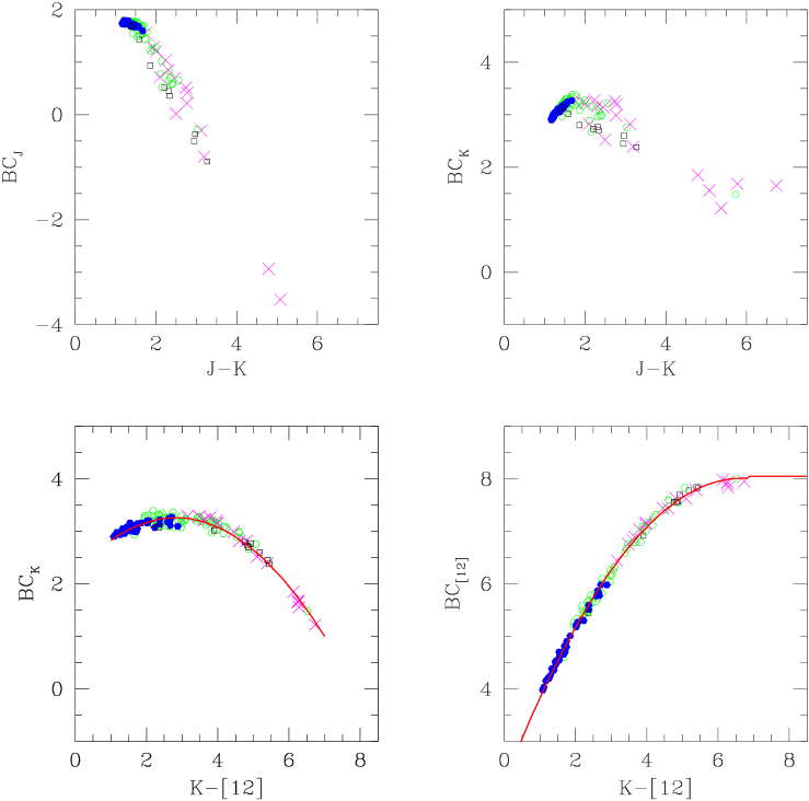
Figure 9: Monitored LPV stars - Bolometric corrections as a function of various colours. Filled circles represent LPV stars in the solar vicinity detected by Hipparcos (Whitelock et al. 2000); open circles represent LPV stars in the Southern Galactic Cap (Whitelock et al. 1994); crosses indicate local high mass–loss LPV stars (Olivier et al. 2001); squares represent obscured LPV stars in the Large Magellanic Cloud (Whitelock et al. 2003). The IRAS 12$\mu$m magnitude is defined as $[12]=-2.5\log F_{12}[{\rm Jy}]/28.3$.

These two curves are complementary to each other. Practically for ${K}-[12]$ smaller than 4 mag it is better to use $BC_{K}$ due to the flatness of the curve. For ${K}-[12]$ redder than 4 mag $BC_{K}$ decreases steeply with increasing colour, while $BC_{[12]}$ is more stable. The narrowness of ($BC_{K}$,${K}-[12]$) and ($BC_{[12]}$, ${K}-[12]$) sequences also suggests that they do not depend on metallicity; in fact, the Magellanic Clouds objects also follow the same relation. Instead, the ($BC_{K}$, $J-K$) sequence depends on metallicity as found by Frogel & Whitford (e.g. 1987) comparing local stars and bulge stars.

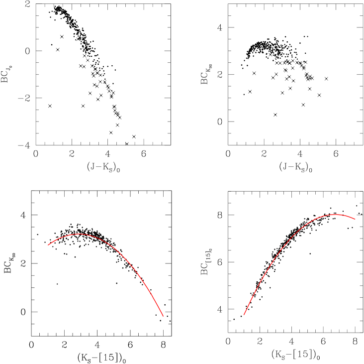
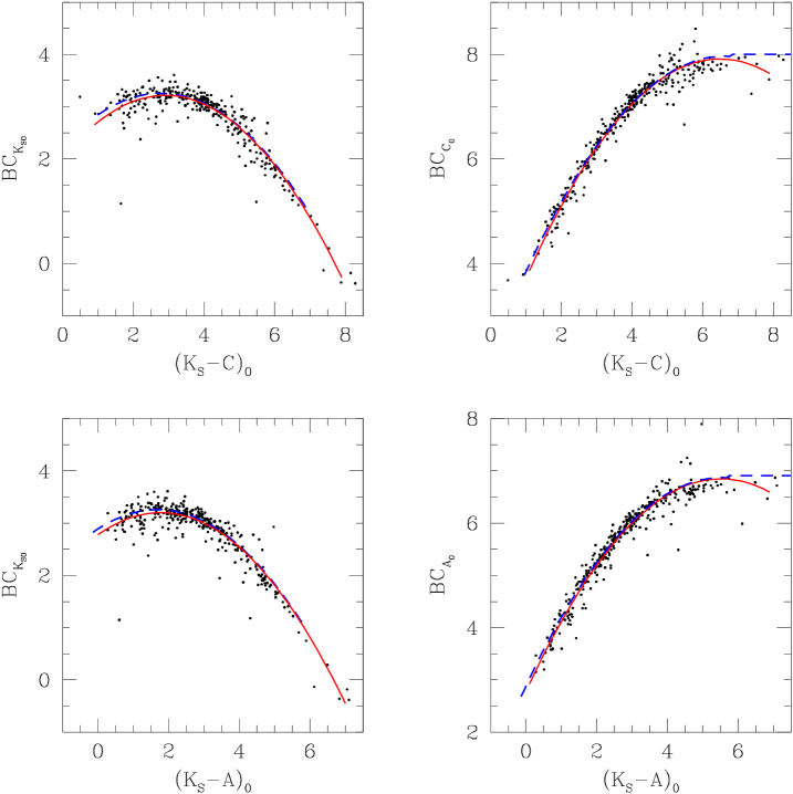
Figure 10: SiO targets - Bolometric corrections versus colours. Crosses are sources with (K_S$-[15])_{0}$ redder than 5 mag. Only sources with bolometric magnitudes well determined are plotted, i.e. when the extrapolation to shorter wavelengths has a negligible contribute to the integrated bolometric magnitude ($<20$%). The 2MASS dataset is plotted. DENIS data are plotted only for sources with poor 2MASS photometry. When both ISOGAL and MSX 15$\mu$m measurement are available, then the average flux density is adopted. Continuous lines indicate our best fits. Dashed lines show the relation found for monitored LPV stars, adapted using the equation $A-[12]=1.15,C-[12]=0.05$ mag (Chapter IV).

2 Bolometric corrections for stars in the inner Galaxy

For the SiO targets we derived bolometric magnitudes as described in Sect. 4.B. Bolometric corrections for the K_S and 15 $\mu$m band are computed from the $m_{\mathrm{bol}}$ and plotted against the dereddened (K_S$-[15])_{0}$ colour in Fig. 10. Identical results are found using separately 2MASS $m_{\mathrm{bol}}$ and K_S or DENIS $m_{\mathrm{bol}}$ and K_S and/or ISOGAL [15] or MSX $D$ (15$\mu$m) band magnitudes. The plotted continuous line is a least–squares polynomial fit, which gives a good match to the data ($\sigma=0.25$ mag) over the range $1.0<$(K_S$-D)_{0}<8.0$:

$$BC_{K_{\rm s}}=2.138+0.745{(K_{\rm s}-[15])_{0}}-0.1294{(K_{\rm s}-[15])_{0}}^{2}.$$

Analogously, using the MSX $A$ (8$\mu$m) band, the following fit is obtained as a function of (K_S$-A)_{0}$ colour in the range $0.0<$(K_S$-A)_{0}>7.0$ ($\sigma=0.25$ mag):

$$BC_{K_{\rm s}}=2.780+0.475{(K_{\rm s}-A)_{0}}-0.1337{(K_{\rm s}-A)_{0}}^{2}.$$

Eventually, using the MSX $C$ (12$\mu$m) band, the following fit is obtained as a function of (K_S$-C)_{0}$ colour in the range $1.0<($K_S$-C)_{0}<8.0$ ($\sigma=0.25$ mag):

$$BC_{K_{\rm s}}=2.037+0.813{(K_{\rm s}-C)_{0}}-0.1398{(K_{\rm s}-C)_{0}}^{2}.$$

The fit to our SiO targets for (K_S$-C)_{0}<2$ mag gives a bolometric correction $BC_{K_{S_{0}}}$ smaller (up to 0.1 mag) than those derived for Hipparcos Mira stars, which have a similar ($K-[12]$) colour. However, within the uncertainty of the fits the two curves derived are consistent.

Chapter 5 Considerations on the dynamics of maser stars in our Galaxy.

Considerations on the kinematics of maser stars

A preliminary report on an ongoing study by
H.J. Habing, M. Messineo, G. van de Ven, M. Sevenster and K.H. Kuijken

Appendix 5.A Introduction

In this thesis we present results from a survey of SiO maser stars undertaken for the explicit reason to investigate stellar kinematics and dynamics in the inner regions of the Milky Way. This survey is a continuation of the thesis project of M. Sevenster in which she looked at 1612 MHz (18cm) for OH/IR stars with the VLA in the northern hemisphere and with the ATCA in the southern hemisphere (Sevenster et al. 1997a, b, 2001). The results of Sevenster’s survey have been presented and analysed in several papers (Sevenster et al. 1999; Sevenster 1999a; Debattista et al. 2002).

In discussing the velocities of the SiO maser stars we came across a question that until now has not been studied in depth: can the line-of-sight velocities ($v_{\mathrm{los}}$) of SiO and OH maser stars in the forbidden quadrants of the longitude-velocity, $(l-v)$, diagram be explained by a rotating bar, and if so, can they be used to constrain the parameters of this bar? A full answer requires two consecutive steps: a) to find a potential and orbits in this potential that will fill the required areas of the $(l-v$) diagram; 2) to find a physical explanation why stars fill these orbits. To answer this question we have started numerical calculations of the orbits in a gravitational potential and compared the predicted longitudes and line-of-sight velocities with those of the observations. Here we describe the first preliminary results of this ongoing study.

Appendix 5.B Available evidence for a Galactic bar

To date, there is clear evidence that the Galactic gravitational field has a weak bar. This was first proposed by de Vaucouleurs (1964) based on the analysis of HI gas velocities and it was later confirmed by, e.g., Binney et al. (1991) and Bissantz et al. (2003). Other evidence comes from the asymmetry around $l=0$ seen in the COBE data (e.g. Blitz & Spergel 1991; Weiland et al. 1994; Binney et al. 1997), star counts (Nakada et al. 1991; Whitelock & Catchpole 1992), and microlensing studies (Paczynski et al. 1994).

Stellar maser emission provides a unique tool for studying stellar kinematics. Unbiased samples of stellar line-of-sight velocities in the inner Galaxy are obtained through stellar OH and SiO maser searches, and these are not affected by interstellar extinction. In this small chapter we focus on the kinematics and spatial distribution of maser stars, whose properties have been discussed in the previous chapters or in the existing literature.

1 Asymmetry in the longitude distribution of maser stars

The data-set resulting from the OH/IR maser surveys by Sevenster et al. (1997a, b, 2001) uniformly covers the entire longitude range from $-45$ to $+45$. It can therefore be used very well to study a possible symmetry in star counts around $l=0$. By plotting $l/|l|$ against $|l|$ in a cumulative fashion, a deviation from (axial) symmetry in the inner Galaxy shows up as a non–horizontal section. In part of the sample $(-10^{\circ}<l<10^{\circ})$ an asymmetry was found that could be explained most naturally by a triaxial (m=2) component in the inner Galaxy, rather than a m=1 asymmetry (Sevenster 1999b). Here we present the same figure of the cumulative distribution (Fig. 1), but for a larger sample of OH/IR stars. The distribution is given for OH/IR stars as well as for MSX sources with AGB colours (as defined in Sevenster 2002) in the same region $(|b|<3$). For OH/IR stars, there is an over-density at negative longitudes close to $l=0$. At larger absolute longitudes, the over-density is at positive longitudes; the slope of the curve is positive. Around $l=40$, the curve seems to level out, but this cannot be assessed in more detail as the sample doesn’t go out far enough.

All these aspects are explained by a bar-like density distribution sampled out to distances well beyond the centre of the Galaxy, up to the far end of the bar. For the MSX sources, the initial negative slope is not seen and the curve starts to rise at lower longitudes. This may be explained by the same bar-like distribution sampled out to smaller distances (for a more detailed discussion see Sevenster 1999b).

Different models used to describe the density distribution of the bar lead to different values of the semi-major axis ($a$) of the bar and the viewing angle ($\phi$), the angle between the line-of-sight and the major axis. However, they do not vary independently, and possible models seem to range very roughly from $\phi=20$ and $a=3$ kpc to $\phi=50$ and $a=2$ kpc; this relation is not necessarily linear. From measurements of the pattern speed (e.g. Debattista et al. 2002) we only have an upper limit for the semi–major axis of about 3 kpc, so it will probably be hard to constrain the viewing angle as described here. However, if some parameters or even the functional form of the bar density are known from other arguments, this will limit the degrees of freedom considerably.

Figure 1: On the horizontal axis the absolute longitude, $|l|$, is displayed and on the vertical axis the cumulative sum of $l/|l|$.

2 Longitude–velocity diagram

We will use three observational $(l-v)$ diagrams. In the top panel of Fig. 2 the CO line spectrum from Dame et al. (2001) is shown; the middle panel shows the OH/IR stars observed by Sevenster and collaborators and the lower panel shows the SiO masers studied in this thesis.

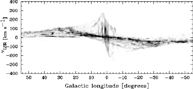
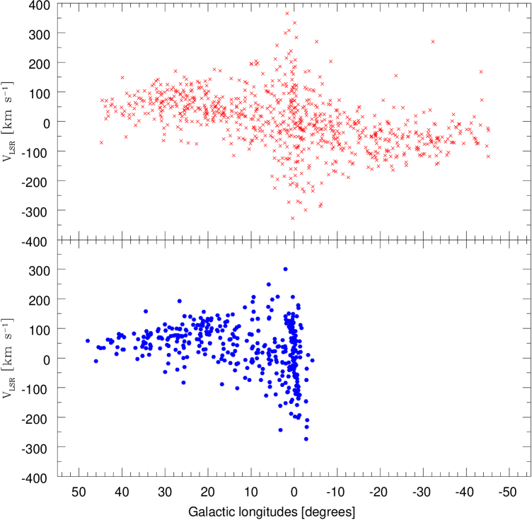
Figure 2: Longitude–velocity diagrams. In the upper panel the CO distribution from Dame et al. (2001) is shown; the middle panel shows the sample of 766 OH/IR stars by Sevenster et al. (1997a, b, 2001); the lower panel shows the distribution of the 271 SiO masing stars from Chapter II plus another $\sim 90$ unpublished SiO maser detections.

If a cloud is located at the tangent point to the line of sight of a circular orbit around the Galactic centre (GC), its velocity vector will point entirely along the line-of-sight; the velocity at the tangent point is the highest velocity seen along a given line-of-sight. It will be called the terminal velocity, $v_{\rm term}$. An analytic relation exists between terminal velocity and longitude: $v_{\rm term}=v_{\rm los}(R_{\rm tang})-V_{\odot}{\rm sin}(l)$. This is plotted in Fig. 3, as two continuous curves, adopting a constant tangential velocity, $V_{\odot}$ of 220 km s^-1, all the way to the GC. The terminal velocity relation gives a good approximation to the highest velocity of the CO gas outside longitudes of about $\pm 20$, confirming that the gas in the Galactic plane moves largely in circular orbits around the GC. Most of the stars appear also constrained by the same curve. However, since stars have higher velocity dispersions than the gas, some stars cross the edge defined by the gas terminal velocity by up to 60 km s^-1.

There is a lower density gas region at positive velocities between longitudes 20 and almost 0 and similarly at negative velocities and longitudes between 0 and $-20$. Gas simulations show that a barred potential explains the gas distribution well, including the low–density regions (Athanassoula & Bureau 1999). Gas on intersecting orbits will collide with itself and a steady flow is not possible. The gas looses angular momentum and it will flow into smaller orbits at lower energies. Holes seem to appear also in the stellar $(l-v)$ diagram of the maser stars, but they can not be explained in the same way.

In the region close to the GC, not only the holes in the gas $(l-v)$ distribution, but also the presence of stars at forbidden velocities in the two quadrants ($l>0$ and $v_{\mathrm{los}}$$<0$) and ($l<0$ and $v_{\mathrm{los}}$$>0$) show that the assumption of circular orbits breaks down. In figure 3, where maser stars are over–plotted on the CO gas, the curve $-V_{\odot}\sin(l)$ is drawn. At positive (negative) longitudes the stars above (below) this curve could move on circular prograde orbits. This apparently applies to all maser stars in the longitude range $345^{\circ}\,>l>\,15^{\circ}$. However, forbidden velocities at longitudes $|l|<15$ are a clear sign of non–circular orbits. Both the OH and the SiO masers populate these regions within pretty much the same boundaries.

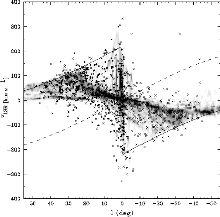
Figure 3: This $(l-v)$ diagram shows the maser stars on the CO map. Symbols are as in Fig. 2. Continuous lines show the expected terminal velocities under the assumption of circular orbits. The dashed line is the curve $-V_{\odot}\sin(l)$, which corresponds to the opposite of the velocity of the Sun along the line-of-sight. At positive (negative) longitudes the stars on circular orbits above (below) this curve are moving prograde in the Galactic standard of rest. The remaining regions are then the forbidden regions.

3 Nuclear Disk

The distribution of gas in the inner one degree from the Galactic centre, the circumnuclear zone (CMZ) or nuclear ring, is well described by a disk with a radius of about 200 pc radius (Morris & Serabyn 1996; Combes 1991). This disc appears in the $(l-v)$ diagram as a distinct feature: a strong correlation between longitude and velocity, at longitudes $-1.4<l<1.5$, with maximum velocities of about 200 km s^-1. Since the gas is a collisional medium, intersecting orbits are forbidden to gas. Dynamical models in a barred potential predict 2 kinds of orbits: X1, along the major axis of the bar, and X2 perpendicular to the X1. When the X1 start to be self–intersecting the gas moves inward in to the lower energy X2 orbits. The transition between the cusped X1 orbit and the X2 appear as a shock region where atomic gas is possibly converted in molecular gas. In principle, stars can populate the intersecting X1 orbits not accessible to gas clouds.

A strong correlation between longitude and velocity is seen also in the maser stars. It was first seen in OH/IR stars within 1 from the GC (Lindqvist et al. 1992; Sjouwerman et al. 1998) and clearly appears in our SiO maser stars (Fig. 2). A linear regression fit using the OH/IR stars gives a slope of $180$ km s^-1 pc^-1 (Lindqvist et al. 1992), consistent with that derived for SiO targets (Chapter V).

As seen in Chapter V, nuclear disk stars are highly obscured (A${}_{\rm K_{\rm S}}$ $>2$ mag). The use of extinction estimates enabled us to exclude possible foreground objects and to select individual stellar members of the nuclear disk. Furthermore, since SiO targets are very bright at near–infrared wavelengths (Chapter III), they are ideal for follow–up spectroscopic studies of the nuclear–disk population.

Appendix 5.C A simple dynamical model

In an axisymmetric potential, the angular momentum of each star, $L=r^{2}\,\partial\phi/\partial t$ is conserved and thus the stars will keep the same direction (i.e. $\partial\phi/\partial t$ will not change sign) when a star moves along its orbit. Clockwise moving stars (i.e. with positive line-of-sight velocity) seen at a positive longitude will move away from us (after correction for LSR motion). At negative longitudes these clockwise rotating stars are all coming toward us (i.e. $v_{\mathrm{los}}$$<0$). In the $(l-v)$–diagram counter rotating stars will appear only in the ”forbidden quadrants” ($l>0$ and $v_{\mathrm{los}}$$<0$) and ($l<0$ and $v_{\mathrm{los}}$$>0$).

Kinematic deviations from what would be expected in an axisymmetric potential were found by Sevenster et al. (2000), when modelling the underlying distribution function (DF). The observed line-of-sight dispersions for instance could not be explained by an axisymmetric model with $\sigma_{R}$ equal to $\sigma_{z}$. Moreover, to explain the stars in the forbidden quadrants, isotropic components had to be invoked.

A barred potential explains the Galactic kinematics well. Several N–body dynamical models of the barred Milky Way exist (e.g. Fux 1997). They can be compared with observations qualitatively, but do not allow a real fit to the data. The latter is possible with the few dynamical models that are built by superposition of either (analytical) DF components (Sevenster et al. 2000) or of numerically integrated orbits (e.g. Häfner et al. 2000; Zhao 1996). The latter method is also known as Schwarzschild’s method and is more general than the DF method, as it does not require a priori assumptions about the form of the DF, which is even more complicated by the fact that $E_{J}$ is the only known integral of motion.

For the population of maser stars, no realistic dynamical model with a barred potential has yet been constructed. Therefore we started to calculate orbits in a barred potential with the ultimate goal to predict the observed distribution of maser points in the $(l-v)$ diagram. This is work under way, but the first results are promising. In the following we briefly sketch the various assumptions and steps made for our calculation and some first results.

1 Geometry

We adopt a Cartesian coordinate system $(x,y,z)$, corotating with the bar–like bulge at a (clockwise) angular speed of $\Omega_{b}=60$ km  s^-1  kpc^-1(Debattista et al. 2002). The origin of the coordinate system is at the Galactic centre, the $x$–axis is aligned with the major axis of the bar–like bulge and the $y$–axis with its minor axis. The Sun is assumed to lie at a distance $R_{\odot}$ from the Galactic centre, in the Galactic plane. The Sun-GC line makes an angle $\phi$ w.r.t. the long–axis of the bulge. We fix the Sun’s distance to the Galactic centre at $R_{\odot}=8$ kpc and its (clockwise) azimuthal velocity to $V_{\odot}=200$ km s^-1. For a given mass model, this leaves two free parameters: the angular speed $\Omega_{b}$ of the bar-like bulge and the angle $\phi$ of the Sun w.r.t. to long–axis of this bulge.

2 Equations of motion

We calculate numerically the orbits of stars in a frame of reference that is rotating in the Galactic plane at an angular speed, $\vec{\Omega_{b}}=(0,0,\Omega_{b})$, solving the equation:

$$\ddot{\mathbf{r}}=-\nabla\Phi_{\mathrm{eff}}-2\left(\mathbf{\Omega_{b}}\times\dot{\mathbf{r}}\right).$$ (1)

In the right–hand side of this equation the first term is the acceleration induced by the effective gravitational potential; the second term is the Coriolis acceleration. The Coriolis acceleration introduces a dependence of the acceleration in the $x$–direction on the velocity in the $y$–direction and vice versa. For further explanations see Binney & Tremaine (1987).

3 Gravitational potential

As a first qualitative study of the stellar dynamics in our Milky Way we consider the non–axisymmetric planar logarithmic potential (Binney & Tremaine 1987)

$$\Phi(x,y)=\frac{1}{2}v_{0}^{2}\ln\left(R_{C}^{2}+x^{2}+\frac{y^{2}}{q^{2}}\right),$$ (2)

with constant velocity $v_{0}$, core radius $R_{C}$ and axial ratio $q\leq 1$. Near the centre ($R\equiv\sqrt{x^{2}+y^{2}}\ll R_{C}$) the logarithmic potential approximates that of a two-dimensional harmonic oscillator, such that the corresponding central density is nearly homogeneous. Going outwards the rotation curve rapidly flattens to $v_{c}\sim v_{0}$. The constant axial ratio implies that the influence of the non–axisymmetry is similar at all radii. Although at larger radii this is not realistic for our Galaxy, the orbits calculated in this rotating potential are still representative as they become nearly circular beyond the corotation radius.

4 First results

Taking the above logarithmic potential with $v_{0}=200$ km s^-1, $R_{C}=0.14$ kpc and $q=0.9$, we calculated a set of closed orbits by numerically solving Eq. (1) with $\Omega_{b}=60$ km  s^-1  kpc^-1. We used a fifth order Runge-Kutta algorithm as described in ”Numerical Recipes” (Press et al. 1992). A representative example of these orbits in the $XY$-plane and in the ($l-v$) diagram, is shown in Fig. 4.

We have just started these simulations and we need to further compare our model to observations in a quantitative way. However, as already proposed by Binney et al. (1991) for the gas, it clearly appears from the simple superposition of the orbits in the $(l-v)$ diagram that orbits from the X1 and X2 families can explain the observed forbidden stellar velocities.

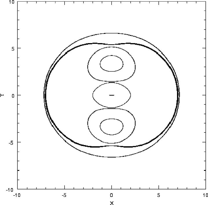
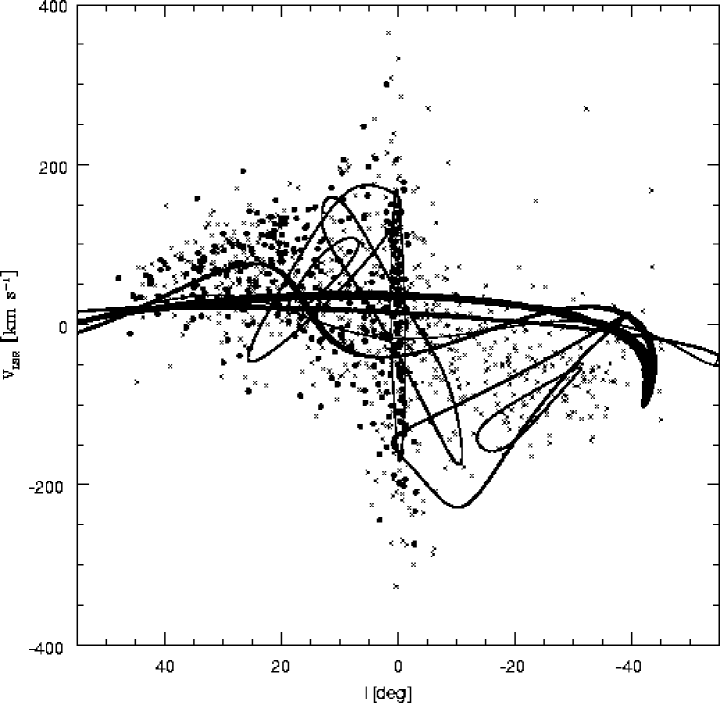
Figure 4: Left panel: $(x,y)$ plot of an example of closed orbits calculated in a rotating logarithmic potential (see text). Right panel: the same orbits projected in a ($l-v$) diagram assuming $\phi=45$.

Appendix 5.D Summary and future plans

In summary, the SiO and OH maser stars have a similar distribution in the velocity-longitude diagram. Their forbidden velocities are difficult to understand in an axisymmetric potential, but they can be understood in a rotating barred potential.

The disk maser stars beyond longitudes $|l|>15$ are probably moving on loop orbits. Outside of the bar region the potential must be close to axisymmetry as observed in the terminal velocities of the gas.

For stars within longitudes $|l|<15$, their forbidden velocities can be explained by X1/X2 orbits.

The most realistic potential currently available is that obtained by the Basel group (Englmaier & Gerhard 1999; Bissantz et al. 2003). This is based on a mass model of the Milky Way derived from the dust corrected COBE maps. We plan to use the Basel potential to calculate a library of orbits and to fit these orbits to the available kinematics of maser stars. The fit can be done by maximising the likelihood of the line-of-sight velocity distribution at the (discrete) observations.

Chapter 6 The ISOGAL survey and the completeness analysis

The ISOGAL survey and the completeness analysis

Appendix 6.A Introduction

The ISOGAL project is an ISO infrared survey of specific regions in the Galactic Plane, which were selected to provide information on Galactic structure, the stellar populations and mass-loss, and the recent star formation history of the inner disk and Bulge of the Galaxy. Several (about 25) scientific papers have been published based on the ISOGAL data. They present studies of the Galactic structure, an analysis of the complete AGB population, and studies of infrared dark clouds and young stellar objects (Omont et al. 2003).

The survey was performed at 7 and 15 $\mu$m with ISOCAM, covering 16 square degrees with a spatial resolution of 3-6and a sensitivity of 10-20 mJy, two orders of magnitude deeper than IRAS at 12$\mu$m, and a factor 10 deeper than the MSX A band (8$\mu$m).

The 7 and 15 $\mu$m ISOGAL data were combined with the $I$, $J$, $K_{s}$ (effective wavelengths 0.79, 1.22 and 2.14 $\mu$m) ground-based data from the DENIS survey, resulting in a 5-wavelength catalogue of point sources. The combination of mid- and near-infrared measurements permits a determination of the nature of the individual sources and of the interstellar extinction towards them.

A complete overview of the first scientific results from ISOGAL data is given by Omont et al. (2003), while the description of the point source catalogue is given in an Explanatory Supplement (Schuller et al. 2003).

In the present chapter I will briefly describe the survey and than I will move to the description of the ISOGAL completeness analysis (Sect. 1.4 below), to which I contributed significantly.

Appendix 6.B Observations

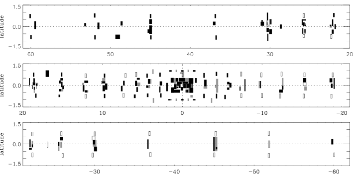
Figure 1: Galactic map of ISOGAL fields with $|\ell|$ $<$ 60^∘. Black, grey and open boxes show fields which have been observed at both 7 & 15 $\mu$m, at 7 $\mu$m only and at 15 $\mu$m only, respectively. Twenty–one additional northern fields (not displayed) were also observed, at $\ell$ $\approx$ +68^∘, +75^∘, +90^∘, +98^∘, +105^∘, +110^∘, +134^∘, +136^∘, & +138^∘. Figure adapted from Schuller et al. (2003).

The ISOGAL observational program –250 hours of observing time– is one of the largest ISO programs. The ISOCAM observations were taken from January 1996 to April 1998, i.e., over the whole ISO mission.

The observed fields ($\sim$16 deg²) are distributed along the inner Galactic Disk, mostly within $|\ell|$ $<$ 30^∘, $|{\it b}|$ $<$ 1^∘, as shown in Figure 1.

Detailed information on the observation parameters and on the field positions is available in the ISOGAL Explanatory Supplement (Schuller et al. 2003) and on the ISOGAL web server www-isogal.iap.fr/.

Most of the observations were performed with the broad filters $LW2$ and $LW3$ and a pixel scale of 6. A few regions around the Galactic centre were observed with the narrow filters $LW5$ or $LW6$, and $LW9$ and a pixel scale of 3, to reduce the effects of bright sources that would saturate the detector (thus moving the saturation limit from $Flux_{12}>6$ Jy to $Flux_{12}>20$ Jy). A list of the ISOCAM filters used for the ISOGAL survey is given in Table 1.

Table 1: ISOCAM filters used for ISOGAL: reference wavelengths and bandwidths, zero point magnitudes and flux densities, and total observed area. Table adapted from Schuller et al. (2003).

Filter	$\lambda_{ref}$	$\Delta\lambda$	ZP	$F_{mag=0}$	Area
	[$\mu m$]	[$\mu m$]	[mag]	[Jy]	[deg2]
LW2	6.7	3.5	12.39	90.36	9.17
LW5	6.8	0.5	12.28	81.66	0.64
LW6	7.7	1.5	12.02	64.27	2.97
LW3	14.3	6.0	10.74	19.77	9.92
LW9	14.9	2.0	10.62	17.70	3.53

The observations, performed in raster mode ($\sim$0.1 deg²), were oriented in Galactic coordinates. At each raster position 19 basic ISOCAM frames (32 x 32 pixels) were taken, resulting in a total integration time of 21 s per raster position. The raster steps were typically 90 in one direction and 150 in the other direction, and each sky point was observed for a maximum of 4 times, with an average of 1.5. Only 384 of the 463 raster positions were used for the production of the first ISOGAL point source catalogue, because only one raster was used in case of overlapping areas to avoid redundancy. The total number of ISOGAL fields (rectangular area of the sky whose edges are aligned with the galactic axes and observed by ISOGAL) is 263. They can be divided in 43 fields (FA) only observed at 7 $\mu$m, 57 fields (FB) only observed at 15 $\mu$m, and 163 fields (FC) observed at both 7 and 15$\mu$m.

Systematic cross-identification with the near-infrared $I,J,K_{\rm s}$ sources of the DENIS survey was an integral part of the ISOGAL program and special DENIS observations were performed for this purpose (Simon 2004). DENIS data were available for 95% of the fields surveyed with ISOCAM.

Appendix 6.C Data processing and analysis

Data reduction was performed with standard procedures of the CAM Interactive Analysis Package (CIA version 3). A sophisticated pipeline was developed for the ISOGAL data (Schuller et al. 2003), which involves more steps than the standard treatment of ISOCAM data (see ISOCAM Handbook, Blommaert et al. 2003). This was necessary because of the extreme conditions of the ISOGAL observations. In addition to the usual problems, i.e. glitches, dead pixels and the time-dependent behaviour of the detectors, one needs also to consider bright background emission, crowding, high spatial density of bright sources (which causes pixel-memory effects), and the short integration time.

The point sources were extracted using a dedicated PSF fitting routine (Schuller et al. 2003).

The completeness of point source extraction has been systematically addressed through retrieval of artificial sources, which is described in the next section.

Appendix 6.D Artificial sources

Synthetically reproducing the complete process of photometric measurements is the only way to properly characterise all undesired effects associated with observations in a crowded field.

An artificial star experiment consists of adding artificial stars to ISOGAL images, and re-extracting all point sources with the same pipeline as the one used to generate the ISOGAL catalogue. The analysis of input magnitudes of artificial sources with those in output enables one to characterise the effects of crowding on the photometric quality and the completeness of the extracted point source catalogue.

Artificial star experiments were conducted on ISOGAL images following a procedure similar to that applied by Bellazzini et al. (2002):

• The magnitude of artificial stars was randomly extracted from the observed luminosity function.

• The goal of the procedure is to study the effects of crowding. Therefore, it is of primary importance that the artificial stars do not interfere with each other. The interference between artificial stars would, in fact, change the actual crowding and affect the results of the artificial experiment study. To avoid this serious bias, one can divide the image (or raster in the ISOGAL case) into grids of cells of known width (20 pixels). One artificial star is randomly positioned in each cell, avoiding the border of the cell in order to control the minimum distance between adjacent artificial stars.

• The stars were simulated using the point-spread-function (PSF) determined directly from the average ISOGAL data corresponding to the observational setup (filter, pixel scale). A new image was then built by adding the artificial stars and their Poisson photon noise into the original raster image.

• The measurements process was performed in the same way as the original measures.

• The output magnitudes were recorded, as well as the positions of the lost stars.

• To generate a significant number of artificial stars, for each image, the whole process was repeated between 100 and $\sim$300 times, depending on the source density and image size. A total of 5$\times$10³ to 4$\times$10⁴ sources were generated.

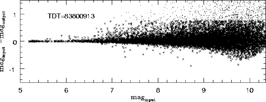
Figure 2: Differences between the input and output magnitudes of the 19250 artificial stars vs. input magnitudes for the raster TDT=83600913. If the difference is larger then 0.75 mag the artificial star is considered lost.

As an example, figure 2 shows the differences between input and output magnitudes, $mag_{input}-mag_{output}$, obtained for the raster TDT=83600913 (filter=$LW2$, pixel scale 6), which is centred at longitudes 1.37 and latitude $-2.63$, covers a region of $0.22\times 0.24$, and has a density of 6660 sources per deg^-2. A number of 55 artificial star were added each run and a total of 350 runs were performed.

The distribution of the difference is not symmetric. There is a strong concentration at zero, but also a positive tail of stars. This means that the output magnitudes are brighter then the input ones and this is due to the blending between artificial stars and real stars. When an artificial star is blended with a fainter source its output magnitude will be brighter than its input magnitude because of the flux contributed by the fainter blended source. Artificial sources having an output magnitude $+$0.75 mag brighter than their input magnitude were considered lost. In fact, if at the position of the artificial star one measures a point source more than 0.75 mag brighter than the magnitude of the input artificial star, this means that the artificial star falls on a brighter real source and in this case the star actually recovered is the real one.

Artificial star simulations were conducted on 35 images (total area $\sim$2 deg²) selected to have all possible observational setups and different crowding levels (the source density ranges from 0.0017 to 0.03 sources per pixel). Artificial star experiments were used to evaluate both random and systematic photometric errors due to crowding, as well as the completeness level of the extraction as a function of source density.

Figure 3: Left-panel: Mean differences between the input and recovered magnitudes per bin of input magnitude, relative to the 19250 artificial stars simulated for the raster TDT=83600913. Right-panel: Standard deviation of the differences between the input and recovered magnitudes as a function of the input magnitude.

Output magnitudes were generally found to be brighter than input magnitudes. This bias is very small for bright stars, but can reach 0.3 magnitude for the faintest ones in the densest fields, where the probability of blending with real stars is higher (see Fig. 3).

The completeness of the extraction was quantified by analysing for each simulation the fraction of retrieved simulated sources as a function of input magnitude. A smooth curve appears which drops at faint magnitudes. The magnitude where this fraction becomes less than 50% depends on the density of the field. The point source catalogues extracted from the various ISOGAL rasters were found at least 50% complete down to the faintest end in fields with low stellar density, but this was not the case in denser regions.

Table 2: Sensitivities at 7 and 15 $\mu$m for typical ISOGAL conditions . Table adapted from Omont et al. (2003).

Region	Source	Background	Pixel	Filter	7 $\mu m$		15 $\mu m$
	density				mag	flux (mJy)	mag	flux (mJy)
A	low	weak	6	broad	10	9	8.7	7
B	high	moderate	6	broad	9	22	8	12
C	very high	strong	3	narrow	8.4	35	7	30
D	high	very strong	6	narrow	7.7	55	6.5	45

Sensitivity limits of ISOGAL sources published in PSC Version 1, corresponding approximately to detection completeness of 50% (Schuller et al. 2003).
Typical regions:
A Lowest density Bulge fields, $|$b$|$ $\geq$ 2^∘
B Standard Disk fields, $|$b$|$ $<$ 0.5^∘, $|$$\ell$$|$ $\leq$ 30^∘
C Central Bulge/Disk fields, $|$b$|$ $<$ 0.3^∘, $|$$\ell$$|$ $\leq$ 1^∘
D Most active star formation regions such as M16, W51.

For each observational setup (combination of pixel scale and filter) a relation between the estimated 50% completeness limit and the field source density was derived and used to define the limiting magnitude of each ISOGAL observation, corresponding to the faintest sources that were included in the published catalogue. The completeness limit depends on the source density, on the intensity and the structure of the local diffuse background, and on the filter. The sensitivities reached at 7 and 15 $\mu$m for standard ISOGAL conditions are summarised in Table 1.

The distribution of limiting magnitudes, for all ISOGAL observations is shown in Fig. 4. Since most observations were done with the broad $LW2$ and $LW3$ filters, these histograms show that the typical reached sensitivity is around 20 mJy at 7 $\mu$m and 12 mJy at 15 $\mu$m.

Figure 4: Distribution of the magnitudes at which the catalogues become incomplete at the 50% level for the broad filters LW2 and LW3 (full lines), and for the narrow filters (dotted lines). The logarithmic scales at the top of each panel show the corresponding flux densities in mJy for LW2 and LW3. A small correction has to be applied for the corresponding flux densities with narrow filters. Figure adapted from Schuller et al. (2003).

About $\approx$25% of extracted point sources fall below these magnitude limits. Analysing the quality flags of discarded sources, the photometric cut is far more severe for moderate quality sources than for good quality ones.

The completeness findings have been complemented and checked by the results of several repeated observations (in one case with 3$\arcsec$ pixels, rather than the typical 6$\arcsec$ pixels, and hence with greatly reduced crowding), and by comparison with DENIS (or 7 $\mu$m) red giant source counts.

Appendix 6.E Concluding remarks

In summary the ISOGAL PSC (version 1.0) contains 106 150 sources. It gives I, J, K_s, [7], [15] magnitudes, at five wavelengths (0.8, 1.25, 2.15, 7 & 15 $\mu$m); DENIS associations (I,J,K_s) are given when available. About half of the sources have 7-15 $\mu$m associations and 78% have DENIS associations. Quality flags are provided for each source at each wavelength, as well as for source associations, and only sources with a reasonable quality and with a magnitude above the 50% completeness limit are included in the catalogue (Schuller et al. 2003).

Op een heldere avond kunnen we aan de hemel een witte, op sommige plekken onderbroken band van licht tegenkomen. Wat we zien zijn miljoenen sterren die samen de schijf van ons eigen sterrenstelsel, de Melkweg, vormen. De Melkweg is opgebouwd uit een enorme bolvormige halo die grotendeels uit donkere materie bestaat, verder een grote, vlakke schijf van gas en sterren, en in het midden van de Melkweg bevindt zich een verdikking in de schijf, de lens (zie fig. 1). Sterren in de schijf van de Melkweg draaien rond het centrum, waarvan we nu weten dat het een zwart gat bevat. Hoe dichter een ster bij het centrum staat, des te korter is de tijd die het de ster kost om één keer rond te gaan. De zon bevindt zich op een afstand van ongeveer 26.000 lichtjaren van het centrum van de Melkweg en beweegt met een snelheid van zo’n 220 km per seconde rond het centrum. Zelfs met deze snelheid kost het ons zonnestelsel rond de 226 miljoen jaar om één keer rond het centrum van de Melkweg te gaan.
Het bestuderen van onze Melkweg is belangrijk voor ons begrip van de vorm, het ontstaan en de ontwikkeling van sterrenstelsels in het algemeen. De structuur en dynamica van het gas en de sterren die deel uit maken van de Melkweg kunnen door hun relatieve nabijheid (vergeleken met andere sterrenstelsels) in groot detail worden bestudeerd. Maar omdat wij ons ook zelf in de Melkweg bevinden krijgen we te maken met projectie-effecten die het ons lastig maken om de grote schaal structuur van de Melkweg te achterhalen.

De Melkweg: een spiraalstelsel met een balk in het centrum

De sterren en het gas in de schijf van de Melkweg liggen gegroepeerd in vier spiraalarmen. Wijzelf bevinden ons aan de rand van de Orion spiraalarm, tussen de Sagittarius arm en de Perseus arm in.

Over het algemeen is de lens in het centrale deel van een sterrenstelsel ofwel bolvormig, net als een bal, of uitgerekt tot een balk, waarbij de spiraalarmen aan de uiteinden van de balk ontstaan. De beweging van zowel gas als sterren geeft aan dat zich in het centrum van de Melkweg een balk bevindt. Ofschoon we tegenwoordig overtuigd zijn van het bestaan van deze balk in het centrum van de Melkweg, weten we nog nauwelijks iets af van zijn eigenschappen, zoals zijn lengte en dikte, of de hoek waaronder we de balk zien.

Figure 5: Deze afbeelding gemaakt met de COBE satelliet laat zien hoe onze Melkweg eruit ziet in het nabij-infrarode deel van het spectrum, waar het meeste licht afkomstig is van geëvolueerde sterren genaamd rode reuzen. De extinctie door interstellair stof is veel zwakker op infrarode golflengten dan op golflengten in het zichtbare deel van het spectrum. Door nu juist op deze golflengten te kijken kunnen we ons dus een veel beter beeld vormen van de Melkweg.

Interstellaire extinctie

Een van de grootste problemen die we tegenkomen bij het bestuderen van de structuur van onze Melkweg is de verduistering door interstellair stof die sterker wordt naarmate we dichter bij het centrum van de Melkweg komen. Interstellair stof dat zich langs de gezichtslijn bevindt absorbeert en verstrooit het licht afkomstig van de sterren die we waarnemen. Dit effect genaamd extinctie (of ’uitdoving’) zwakt de helderheid van de ster af en het maakt het spectrum van het sterlicht roder. Het sterspectrum laat zien hoe het licht afkomstig van de ster verdeeld is over de verschillende golflengten. Voor licht in het zichtbare deel van het spectrum is de extinctie zeer hoog, maar voor langere golflengten, zoals in het nabije- en mid-infrarode deel van het spectrum, is de extinctie minder sterk (zie fig. 2). Op infrarode golflengten kunnen we dus een veel duidelijker beeld krijgen van onze Melkweg. In de afgelopen tien jaar zijn verschillende onderzoeken (surveys) uitgevoerd op infrarode golflengten om de structuur en de vormingsgeschiedenis van onze Melkweg te achterhalen. Deze data bevat een schat aan informatie over de opbouw van sterpopulaties die er nog op wacht om volledig geanalyseerd te worden.

Dit promotie-onderzoek gaat over de bepaling van de structuur en samenstelling van de binnenste delen van onze Melkweg, daarbij gebruik makend van geëvolueerde sterren (sterren die al het grootste deel van hun leven achter de rug hebben) om het zwaartekrachtsveld in dit deel van de Melkweg in kaart te brengen. Het zwaartekrachtsveld kan ons namelijk meer vertellen over de verdeling van massa in de Melkweg.

Geëvolueerde sterren en de massaverdeling en kinematica van de Melkweg

De meeste sterren die we kunnen zien op infrarode golflengten zijn geëvolueerde reuzesterren, koude (rode) sterren die aan hun oppervlakte typisch zo’n 3000 K warm zijn (ter vergelijking: onze zon heeft een oppervlaktemperatuur van zo’n 6000 K!). Wij noemen ze reuzesterren vanwege hun grote omvang: als de zon een reuzester is geworden zal haar straal groter zijn dan de aardbaan. De sterren waar we het hier over hebben zijn ongeveer even zwaar of wat zwaarder dan onze eigen zon (tot zo’n 6 keer zo zwaar). Ofschoon deze sterren relatief koud zijn voor sterbegrippen zijn ze toch heel helder: typisch 3000 keer helderder dan onze zon. Rode reuzen verbranden waterstof en/of helium in een schil rond hun kern. Hun leeftijd ligt tussen de 1 en de 15 miljard jaar; ze zijn bijna aan het eind van hun leven aangekomen.

Geëvolueerde sterren hebben sterke winden die de ster omhullen met een mantel van gas en stof. De aanwezigheid van stof is vastgesteld uit een overschot aan infrarood licht dat van deze sterren afkomt. Stof absorbeert namelijk licht afkomstig van de ster en zendt dit weer uit op (voornamelijk) infrarode golflengten. We weten dat zich ook gas in de mantel rond deze sterren moet bevinden omdat we straling meten die wordt uitgezonden door sommige moleculen (zoals CO) op golflengten van een millimeter of iets minder dan een millimeter. Deze circumstellaire mantels zenden bovendien vaak maserstraling uit (het equivalent van laserstraling maar dan in het millimeter deel van het spectrum), afkomstig van moleculen zoals OH, SiO en H₂O (water). We kunnen deze maserstraling opvangen uit alle delen van de Melkweg. De golflengte van deze maserlijnen lijkt in de waarnemingen verschoven ten gevolge van het Doppler effect, hetzelfde effect waardoor een naderende ambulance een hogere toon lijkt te hebben dan één die weg rijdt. Daarom kunnen we door heel nauwkeurig de golflengte van de maser-emissie te meten de snelheid van deze sterren langs de gezichtslijn bepalen.

Geëvolueerde reuzesterren die helder zijn op infrarode golflengten zijn vanwege bovenstaande redenen uitermate geschikt om de geschiedenis, de structuur en de kinematica (de beweging van o.m. sterren) van de Melkweg te achterhalen. Deze sterren zijn gevormd op verschillende tijdstippen in de geschiedenis van de Melkweg, zoals blijkt uit hun onderlinge leeftijdsverschillen, waardoor zij ons in staat stellen om meer te weten te komen over stervorming in verschillende perioden van het bestaan van de Melkweg. Hun ruimtelijke verdeling wordt bepaald door het zwaartekrachtsveld van de Melkweg, daarom kunnen wij hen ook gebruiken om de massaverdeling die dit zwaartekrachtsveld in de Melkweg veroorzaakt te bepalen. Tenslotte kan de maser-emissie in deze sterren worden gebruikt om nauwkeurig de snelheden van deze sterren te achterhalen, waardoor ze heel goed bruikbaar zijn om de kinematica van de Melkweg te bestuderen.

Onze survey van SiO masers

In dit promotie-onderzoek hebben wij gegevens geanalyseerd uit verschillende surveys in het infrarood, en wij hebben ook SiO maserlijnen waargenomen rond geëvolueerde reuzesterren. De twee hoofddoelen van dit onderzoek zijn ten eerste het bepalen van de snelheid langs de gezichtslijn van de waargenomen sterren en ten tweede het bepalen van de massaverdeling van sterren in de binnenste delen van onze Melkweg. Eigenschappen van geëvolueerde sterren, zoals hun helderheid en massaverlies, kunnen ons verder iets vertellen over de voorwaarden waaronder masers in dit type sterren voorkomen.

Overzicht van dit proefschrift

We hebben gezocht naar SiO maserstraling afkomstig van sterren die in het infrarode deel van het spectrum helder zijn. Het resultaat was dat we het aantal van deze sterren (en daarmee ook hun snelheid langs de gezichtslijn) dat bekend was in de binnenste delen van de Melkweg bijna hebben kunnen verdubbelen. In hoofdstuk 2 tonen we ons onderzoek dat is uitgevoerd met de IRAM 30 meter telescoop, die zich op de Pico Veleta in Spanje bevindt. De sterren die we selecteerden hebben dezelfde kleur als geëvolueerde sterren en bovendien verandert hun helderheid op een periodieke manier. We hebben deze criteria gebruikt omdat al bekend was dat maser-emissie vaker voorkomt bij dergelijke sterren. We vonden SiO masers in 271 van de onderzochte sterren, waarmee het aantal snelheden dat is bepaald voor sterren in de binnenste delen van de Melkweg met behulp van maser lijnen is verdubbeld.

De verdeling van energie van deze sterren over de verschillende golflengtegebieden (afgeleid uit de helderheid van de sterren in het nabije- en mid-infrarode deel van het spectrum) kan worden gebruikt om de helderheid en het massaverlies van deze sterren te bepalen. In hoofdstuk 3 presenteren wij de helderheid van de 441 sterren die we hebben onderzocht op maserstraling op golflengten tussen 1$\mu$men 25$\mu$m(ter vergelijking: het licht dat we met onze ogen zien heeft golflengten tussen de 0.4$\mu$men 0.8$\mu$m) . Metingen gedaan op verschillende tijdstippen laten zien dat de meeste van deze bronnen in helderheid variëren. Hun kleur lijkt op die van veranderlijke geëvolueerde sterren in de zonsomgeving waarvan we weten dat ze worden omgeven door een dunne mantel.

Om de intrinsieke helderheid van een ster te kunnen bepalen moeten we corrigeren voor interstellaire extinctie. We doen dit door de verdeling in het kleur-magnitude diagram (fig. 3) van de door ons waargenomen geëvolueerde sterren te vergelijken met de verdeling in het kleur-magnitude diagram van geëvolueerde sterren waarvan we de extinctie kennen. In hoofdstuk 4 voeren we deze analyse uit, om daarmee de extinctie voor al onze SiO maserbronnen in de verschillende delen van de Melkweg te bepalen. Uit onze analyse volgen ook nieuwe, interessante waarden voor de interstellaire extinctie op verschillende golflengten.

In hoofdstuk 5 berekenen we de intrinsieke helderheid van onze SiO sterren. Als we aannemen dat alle sterren die minder dan 5^∘ van het Melkwegcentrum af staan dezelfde afstand tot de zon hebben, dan vinden we dat de piek in de helderheidsverdeling van onze sterren samenvalt met de piek in de verdeling van geëvolueerde sterren met OH maser emissie die zich in de buurt van het Melkwegcentrum bevinden (deze piek ligt bij ongeveer 8000 keer de helderheid van de zon). Onze data laat zien dat het belangrijkste verschil tussen sterren met OH masers en sterren met SiO masers is dat sterren met OH masers meer massa verliezen per jaar dan sterren met SiO masers. Sterren met SiO masers zijn echter makkelijker waar te nemen op golflengten in het nabij-infrarood dan sterren met OH masers, waardoor het makkelijker is om sterren met SiO masers te gebruiken om meer te weten te komen over de sterren in het midden van de circumstellaire mantel.

Een voorlopige bespreking van de banen van onze SiO maser sterren en een opzet voor onderzoek dat we in de toekomst willen doen wordt besproken in hoofdstuk 6. De beweging van de SiO maser sterren bevestigt het bestaan van een balk in het centrale deel van onze Melkweg. We zijn begonnen met een volledige analyse van de dynamica van onze sterren met als doel het verfijnen van de parameters die de balk beschrijven.

Tenslotte beschrijven we in hoofdstuk 7 in het kort de ISOGAL survey, een survey in het mid-infrarood van het vlak van de Melkweg, maar voornamelijk in de richting van het Galactisch centrum. Deze survey is uitgevoerd om de structuur van de Melkweg te bepalen, in het bijzonder in gebieden in het centrum van de Melkweg en in gebieden waar de interstellaire extinctie groot is. Het is erg lastig om van afzonderlijke sterren de positie en helderheid te bepalen om daarmee een betrouwbare catalogus samen te stellen. In dit hoofdstuk beschrijven wij simulaties die gebruikt kunnen worden om de nauwkeurigheid van helderheden afgeleid uit de ISOGAL afbeeldingen te bepalen.

Biography I am the daughter of Lucia and Leonardo Messineo; sister of Celestina and Saro. I was born at 2 o’clock on a starry night in a place called Salinella, high in the Sicilian mountains. From there in the night you almost always see many stars, but my grandmother told me not to count them because one could never finish. I attended elementary school in Petralia Soprana and intermediate and high school in Bagheria. I began studying Astronomy at the University of Bologna in the fall of 1989. I graduated on March 21st 1997 cum laude with a thesis entitled ”the mixing problem in stellar evolution and the primordial He abundance determination from population ratios in globular clusters”, which I did under the supervision of Prof. Francesco Ferraro from Bologna University and Prof. Flavio Fusi Pecci from the Bologna Observatory. In 1998 I went to Baltimore for six months as a summer student to work at the Space Telescope Science Institute with Dr. Antonella Nota on ISO data of LBV stars. In 1999 I worked at the Bologna Observatory on HST photometry of the globular cluster NGC 288 in collaboration with Dr. Michele Bellazzini. On December 1st 1999, I started my PhD research in Leiden under the supervision of Prof. Harm Habing. For the first year I worked on the ISOGAL catalogue, after which my research turned to late-type stars in the inner Galaxy. This work has been done in collaboration mainly with Prof. Harm Habing, Prof. Karl Menten from the Max-Planck-Institut fuer Radioastronomie in Bonn, Prof. Alain Omont from the Institut d’Astrophysique de Paris and Dr. Lorant Sjouwerman from the National Radio Astronomy Observatory in Socorro. During the past four years I have enjoyed observing with the IRAM 30m telescope in Spain four times as well as with the Heinrich Hertz Telescope in Arizona, with the ESO 3.6m and the CTIO 4m telescopes in Chile. I spent some weeks visiting the Institut d’Astrophysique de Paris, ESA in Villafranca del Castillo, Spain, and the CTIO in La Serena, Chile. I attended the YERAC 2000 school in Granada (Spain), the NOVA 2000 school in Dwingeloo (The Netherlands), and conferences in Angra dos Reis (Brazil), Sendai (Japan) and Kona (Hawaii). I gave invited presentations at the Max-Planck-Institut fuer Radioastronomie in Bonn (Germany), and at the Stichting Astronomisch Onderzoek in Nederland (ASTRON) in Dwingeloo. In September 2004 I will start working as a fellow at ESO in Garching (Germany).

The list of people I have interacted with, learnt from and spent time with during my PhD at Leiden Observatory is very long, and I apologise if I do not mention you all here.

During my first year Wing Fai was still in Leiden, always willing to answer my technical questions. Maria Rosa, Wouter, Inga, Garrelt, Pedro, Petra, Dominic, Yvonne and I were Harm’s group and we used to have a group meeting every Friday, but someone would always complain because the two Italian girls would speak too long!! I spent a lot of time with Roderik, Dominic and Jes, being my officemates and I thank you for being so patient with me.

I used to visit the office of the computer group, which was next to mine, at least once per day reporting obscure behaviours of my computer and I am grateful to David, Tycho, Erik and Aart for always being very helpful. And the management assistants were always great! in particular I had the pleasure to work closely with Kirsten in organising the AGB workshop.

I had the privilege to work with wonderful people and great scientists, among them Karl, Alain, Lorant and Maartje: thanks for your support.

In the past months it has been a great pleasure to start working with Glenn on stellar dynamics and to create the ROTBAAN consortium!

I am indebted to Kirsten, Melanie and Frank for their careful reading of my manuscripts and to Dominic for translating the summary of this document into Dutch.

My numerous changes of apartments brought me to very close friendships with Maria Rosa, Petra, Emanuela and Elena, with whom I have shared so many cups of good coffee and tea.

Infine vorrei ringraziare particolarmente la mia famiglia per avermi incoraggiato nei miei studi e per aver sempre accettato tutte le mie scelte e la mia lontananza.

Grazie tanto!

Bedankt iedereen!

References

- Beaulieu et al. (2000) Beaulieu, S. F., Freeman, K. C., Kalnajs, A. J., Saha, P., & Zhao, H. 2000, AJ, 120, 855
- Binney et al. (1991) Binney, J., Gerhard, O. E., Stark, A. A., Bally, J., & Uchida, K. I. 1991, MNRAS, 252, 210
- Dame et al. (2001) Dame, T. M., Hartmann, D., & Thaddeus, P. 2001, ApJ, 547, 792
- Debattista et al. (2002) Debattista, V. P., Gerhard, O., & Sevenster, M. N. 2002, MNRAS, 334, 355
- Deguchi et al. (2000a) Deguchi, S., Fujii, T., Izumiura, H., et al. 2000a, ApJS, 130, 351
- Deguchi et al. (2000b) Deguchi, S., Fujii, T., Izumiura, H., et al. 2000b, ApJS, 128, 571
- Elitzur (1992) Elitzur, M. 1992, ARA&A, 30, 75
- Feast et al. (1989) Feast, M. W., Glass, I. S., Whitelock, P. A., & Catchpole, R. M. 1989, MNRAS, 241, 375
- Fux (1999) Fux, R. 1999, A&A, 345, 787
- Ghez et al. (2000) Ghez, A. M., Morris, M., Becklin, E. E., Tanner, A., & Kremenek, T. 2000, Nature, 407, 349
- Gilmore & Reid (1983) Gilmore, G. & Reid, N. 1983, MNRAS, 202, 1025
- Gilmore et al. (2002) Gilmore, G., Wyse, R. F. G., & Norris, J. E. 2002, ApJ, 574, L39
- Habing (1996) Habing, H. J. 1996, A&A Rev., 7, 97
- Helmi et al. (1999) Helmi, A., White, S. D. M., de Zeeuw, P. T., & Zhao, H. 1999, Nature, 402, 53
- Ibata et al. (1994) Ibata, R. A., Gilmore, G., & Irwin, M. J. 1994, Nature, 370, 194
- Iben (1985) Iben, I. 1985, QJRAS, 26, 1
- Izumiura et al. (1999) Izumiura, H., Deguchi, S., Fujii, T., et al. 1999, ApJS, 125, 257
- Launhardt et al. (2002) Launhardt, R., Zylka, R., & Mezger, P. G. 2002, A&A, 384, 112
- Lewis (1989) Lewis, B. M. 1989, ApJ, 338, 234
- McWilliam & Rich (1994) McWilliam, A. & Rich, R. M. 1994, ApJS, 91, 749
- Omont et al. (2003) Omont, A., Gilmore, G. F., Alard, C., et al. 2003, A&A, 403, 975
- Reid & Menten (1997) Reid, M. J. & Menten, K. M. 1997, ApJ, 476, 327
- Reid & Moran (1988) Reid, M. J. & Moran, J. M. 1988, in Galactic and Extragalactic Radio Astronomy, 255–294
- Schödel et al. (2003) Schödel, R., Ott, T., Genzel, R., et al. 2003, ApJ, 596, 1015
- Schuller et al. (2003) Schuller, F., Ganesh, S., Messineo, M., et al. 2003, A&A, 403, 955
- Sevenster (1999) Sevenster, M. N. 1999, MNRAS, 310, 629
- Sevenster et al. (1997a) Sevenster, M. N., Chapman, J. M., Habing, H. J., Killeen, N. E. B., & Lindqvist, M. 1997a, A&AS, 122, 79
- Sevenster et al. (1997b) Sevenster, M. N., Chapman, J. M., Habing, H. J., Killeen, N. E. B., & Lindqvist, M. 1997b, A&AS, 124, 509
- Sevenster et al. (2001) Sevenster, M. N., van Langevelde, H. J., Moody, R. A., et al. 2001, A&A, 366, 481
- Wyse et al. (1997) Wyse, R. F. G., Gilmore, G., & Franx, M. 1997, ARA&A, 35, 637

References

- Alard et al. (2001) Alard, C., Blommaert, J. A. D. L., Cesarsky, C., et al. 2001, ApJ, 552, 289
- Bertelli et al. (1994) Bertelli, G., Bressan, A., Chiosi, C., Fagotto, F., & Nasi, E. 1994, A&AS, 106, 275
- Blommaert et al. (2003) Blommaert, J. A. D. L., Siebenmorgen, R., Coulais, A., et al., eds. 2003, The ISO Handbook, Volume II - CAM - The ISO Camera
- Cardelli et al. (1989) Cardelli, J. A., Clayton, G. C., & Mathis, J. S. 1989, ApJ, 345, 245
- Carpenter (2001) Carpenter, J. M. 2001, AJ, 121, 2851
- Carter (1990) Carter, B. S. 1990, MNRAS, 242, 1
- Cioni et al. (2003) Cioni, M.-R. L., Blommaert, J. A. D. L., Groenewegen, M. A. T., et al. 2003, A&A, 406, 51
- Cotera et al. (2000) Cotera, A. S., Simpson, J. P., Erickson, E. F., et al. 2000, ApJS, 129, 123
-
Cutri et al. (2003)
Cutri, C. M., Skrutskie, M. F., & Van Dyk, S. 2003, avalaible on line at
http://www.ipac.caltech.edu/2mass/ - Draine & Lee (1984) Draine, B. T. & Lee, H. M. 1984, ApJ, 285, 89
- Drimmel et al. (2003) Drimmel, R., Cabrera-Lavers, A., & López-Corredoira, M. 2003, A&A, 409, 205
- Dutra et al. (2002) Dutra, C. M., Santiago, B. X., & Bica, E. 2002, A&A, 381, 219
- Dutra et al. (2003) Dutra, C. M., Santiago, B. X., Bica, E. L. D., & Barbuy, B. 2003, MNRAS, 338, 253
- Egan et al. (1999) Egan, M. P., Price, S. D., Moshir, M. M., et al. 1999, AFRL-VS-TR-1999, 1522
- Epchtein et al. (1994) Epchtein, N., de Batz, B., Copet, E., et al. 1994, Ap&SS, 217, 3
- Ferraro et al. (1999) Ferraro, F. R., Messineo, M., Fusi Pecci, F., et al. 1999, AJ, 118, 1738
- Figer et al. (2004) Figer, D. F., Rich, R. M., Kim, S. S., Morris, M., & Serabyn, E. 2004, ApJ, 601, 319
- Fluks et al. (1994) Fluks, M. A., Plez, B., The, P. S., et al. 1994, A&AS, 105, 311
- Fouque et al. (1992) Fouque, P., Le Bertre, T., Epchtein, N., Guglielmo, F., & Kerschbaum, F. 1992, A&AS, 93, 151
- Frogel et al. (1999) Frogel, J. A., Tiede, G. P., & Kuchinski, L. E. 1999, AJ, 117, 2296
- Frogel & Whitford (1987) Frogel, J. A. & Whitford, A. E. 1987, ApJ, 320, 199
- Girardi et al. (2000) Girardi, L., Bressan, A., Bertelli, G., & Chiosi, C. 2000, A&AS, 141, 371
- Glass (1999) Glass, I. S. 1999, Book Review: Handbook of infrared astronomy (Cambridge U. Press)
- Glass et al. (1995) Glass, I. S., Whitelock, P. A., Catchpole, R. M., & Feast, M. W. 1995, MNRAS, 273, 383
- Groenewegen & de Jong (1993) Groenewegen, M. A. T. & de Jong, T. 1993, A&A, 267, 410
- Guglielmo et al. (1993) Guglielmo, F., Epchtein, N., Le Bertre, T., et al. 1993, A&AS, 99, 31
- He et al. (1995) He, L., Whittet, D. C. B., Kilkenny, D., & Spencer Jones, J. H. 1995, ApJS, 101, 335
- Hennebelle et al. (2001) Hennebelle, P., Pérault, M., Teyssier, D., & Ganesh, S. 2001, A&A, 365, 598
- Ivezíc et al. (1999) Ivezíc, Z., Nenkova, M., & Elitzur, M. 1999, User Manual for DUSTY (Lexington: Univ. Kentucky)
- Jeong et al. (2003) Jeong, K. S., Winters, J. M., Le Bertre, T., & Sedmayr, E. 2003, Proceeding of WS on Mass-Losing Pulsating Stars and their Circumstellar Matter, Sendai, Japan, Y.Nakada & M.Honma (eds), Kluwer ASSL series
- Jiang et al. (2003) Jiang, B. W., Omont, A., Ganesh, S., Simon, G., & Schuller, F. 2003, A&A, 400, 903
- López-Corredoira et al. (2002) López-Corredoira, M., Cabrera-Lavers, A., Garzón, F., & Hammersley, P. L. 2002, A&A, 394, 883
- Landini et al. (1984) Landini, M., Natta, A., Salinari, P., Oliva, E., & Moorwood, A. F. M. 1984, A&A, 134, 284
- Lutz (1999) Lutz, D. 1999, in ESA SP-427: The Universe as Seen by ISO, Vol. 427, 623
- Lutz et al. (1996) Lutz, D., Feuchtgruber, H., Genzel, R., et al. 1996, A&A, 315, L269
- Mathis (1990) Mathis, J. S. 1990, ARA&A, 28, 37
- Mathis (1998) —. 1998, ApJ, 497, 824
- McWilliam & Rich (1994) McWilliam, A. & Rich, R. M. 1994, ApJS, 91, 749
- Messineo et al. (2004a) Messineo, M., Habing, H. J., Menten, K. M., Omont, A., & Sjouwerman, L. O. 2004a, A&A in preparation (Chapter V)
- Messineo et al. (2004b) —. 2004b, A&A, 418, 103 (Chapter III)
- Messineo et al. (2002) Messineo, M., Habing, H. J., Sjouwerman, L. O., Omont, A., & Menten, K. M. 2002, A&A, 393, 115 (Chapter II)
- Ojha et al. (2003) Ojha, D. K., Omont, A., Schuller, F., et al. 2003, A&A, 403, 141
- Olivier et al. (2001) Olivier, E. A., Whitelock, P., & Marang, F. 2001, MNRAS, 326, 490
- Omont et al. (2003) Omont, A., Gilmore, G. F., Alard, C., et al. 2003, A&A, 403, 975
- Price et al. (2001) Price, S. D., Egan, M. P., Carey, S. J., Mizuno, D. R., & Kuchar, T. A. 2001, AJ, 121, 2819
- Rieke & Lebofsky (1985) Rieke, G. H. & Lebofsky, M. J. 1985, ApJ, 288, 618
- Rosenthal et al. (2000) Rosenthal, D., Bertoldi, F., & Drapatz, S. 2000, A&A, 356, 705
- Schuller et al. (2003) Schuller, F., Ganesh, S., Messineo, M., et al. 2003, A&A, 403, 955
- Schultheis et al. (1999) Schultheis, M., Ganesh, S., Simon, G., et al. 1999, A&A, 349, L69
- Stanek (1998) Stanek, K. Z. 1998, Using the DIRBE/IRAS All-Sky Reddening Map to Select Low-Reddening Windows Near the Galactic Plane, preprint [astro-ph/9802307]
- Udalski (2003) Udalski, A. 2003, ApJ, 590, 284
- van de Hulst (1946) van de Hulst, H. C. 1946, Optics of spherical particles. (Amsterdam, Drukkerij J. F. Duwaer, 1946.), 1
- van Loon et al. (2003) van Loon, J. T., Gilmore, G. F., Omont, A., et al. 2003, MNRAS, 338, 857
- van Loon et al. (1998) van Loon, J. T., Zijlstra, A. A., Whitelock, P. A., et al. 1998, A&A, 329, 169
- van Loon et al. (1997) —. 1997, A&A, 325, 585
- Vassiliadis & Wood (1993) Vassiliadis, E. & Wood, P. R. 1993, ApJ, 413, 641
- Wainscoat et al. (1992) Wainscoat, R. J., Cohen, M., Volk, K., Walker, H. J., & Schwartz, D. E. 1992, ApJS, 83, 111
- Whitelock et al. (1991) Whitelock, P., Feast, M., & Catchpole, R. 1991, MNRAS, 248, 276
- Whitelock et al. (2000) Whitelock, P., Marang, F., & Feast, M. 2000, MNRAS, 319, 728
- Whitelock et al. (1994) Whitelock, P., Menzies, J., Feast, M., et al. 1994, MNRAS, 267, 711
- Whitelock et al. (2003) Whitelock, P. A., Feast, M. W., van Loon, J. T., & Zijlstra, A. A. 2003, MNRAS, 342, 86
- Winnberg et al. (1991) Winnberg, A., Lindqvist, M., Olofsson, H., & Henkel, C. 1991, A&A, 245, 195

References

- Alcolea et al. (1990) Alcolea, J., Bujarrabal, V., & Gomez-Gonzalez, J. 1990, A&A, 231, 431
- Alcolea et al. (1999) Alcolea, J., Pardo, J. R., Bujarrabal, V., et al. 1999, A&AS, 139, 461
- Bally et al. (1988) Bally, J., Stark, A. A., Wilson, R. W., & Henkel, C. 1988, ApJ, 324, 223
- Baud et al. (1979) Baud, B., Habing, H. J., Matthews, H. E., & Winnberg, A. 1979, A&AS, 35, 179
- Bedijn (1987) Bedijn, P. J. 1987, A&A, 186, 136
- Beichman et al. (1988) Beichman, C. A., Neugebauer, G., Habing, H. J., Clegg, P. E., & Chester, T. J. 1988, in NASA RP-1190, Vol. 1 (1988)
- Binney et al. (1991) Binney, J., Gerhard, O. E., Stark, A. A., Bally, J., & Uchida, K. I. 1991, MNRAS, 252, 210
- Blitz & Spergel (1991) Blitz, L. & Spergel, D. N. 1991, ApJ, 379, 631
- Blommaert et al. (1994) Blommaert, J. A. D. L., van Langevelde, H. J., & Michiels, W. F. P. 1994, A&A, 287, 479
- Burton (1988) Burton, W. B. 1988, in Galactic and Extragalactic Radio Astronomy, 295–358
- Burton & Liszt (1978) Burton, W. B. & Liszt, H. S. 1978, ApJ, 225, 815
- Carter (1990) Carter, B. S. 1990, MNRAS, 242, 1
- Cho et al. (1998) Cho, S., Chung, H., Kim, H., et al. 1998, ApJS, 115, 277
- Cole & Weinberg (2002) Cole, A. A. & Weinberg, M. D. 2002, ApJ, 574, L43
-
Cutri et al. (2003)
Cutri, C. M., Skrutskie, M. F., & Van Dyk, S. 2003, avalaible on line at
http://www.ipac.caltech.edu/2mass/ - de Vaucouleurs (1964) de Vaucouleurs, G. 1964, in IAU Symp. 20: The Galaxy and the Magellanic Clouds, 195
- Deguchi et al. (2000a) Deguchi, S., Fujii, T., Izumiura, H., et al. 2000a, ApJS, 130, 351
- Deguchi et al. (2000b) —. 2000b, ApJS, 128, 571
- Drimmel et al. (2003) Drimmel, R., Cabrera-Lavers, A., & López-Corredoira, M. 2003, A&A, 409, 205
- Egan et al. (1999) Egan, M. P., Price, S. D., Moshir, M. M., et al. 1999, AFRL-VS-TR-1999, 1522
- Englmaier & Gerhard (1999) Englmaier, P. & Gerhard, O. 1999, MNRAS, 304, 512
- Epchtein et al. (1994) Epchtein, N., de Batz, B., Copet, E., et al. 1994, Ap&SS, 217, 3
- Feast et al. (1989) Feast, M. W., Glass, I. S., Whitelock, P. A., & Catchpole, R. M. 1989, MNRAS, 241, 375
- Feltzing & Gilmore (2000) Feltzing, S. & Gilmore, G. 2000, A&A, 355, 949
- Ferraro et al. (2000) Ferraro, F. R., Montegriffo, P., Origlia, L., & Fusi Pecci, F. 2000, AJ, 119, 1282
- Frogel & Whitford (1987) Frogel, J. A. & Whitford, A. E. 1987, ApJ, 320, 199
- Girardi et al. (2000) Girardi, L., Bressan, A., Bertelli, G., & Chiosi, C. 2000, A&AS, 141, 371
- Glass et al. (2001) Glass, I. S., Matsumoto, S., Carter, B. S., & Sekiguchi, K. 2001, MNRAS, 321, 77
- Glass et al. (1995) Glass, I. S., Whitelock, P. A., Catchpole, R. M., & Feast, M. W. 1995, MNRAS, 273, 383
- Groenewegen & de Jong (1993) Groenewegen, M. A. T. & de Jong, T. 1993, A&A, 267, 410
- Guarnieri et al. (1997) Guarnieri, M. D., Renzini, A., & Ortolani, S. 1997, ApJ, 477, L21
- Habing (1996) Habing, H. J. 1996, A&A Rev., 7, 97
- Haikala (1990) Haikala, L. K. 1990, A&AS, 85, 875
- Hughes & Wood (1990) Hughes, S. M. G. & Wood, P. R. 1990, AJ, 99, 784
- Iben & Renzini (1983) Iben, I. & Renzini, A. 1983, ARA&A, 21, 271
- Imai et al. (2002) Imai, H., Deguchi, S., Fujii, T., et al. 2002, PASJ, 54, L19
- Izumiura et al. (1999) Izumiura, H., Deguchi, S., Fujii, T., et al. 1999, ApJS, 125, 257
- Josselin et al. (1996) Josselin, E., Loup, C., Omont, A., Barnbaum, C., & Nyman, L.-A. 1996, A&A, 315, L23
- Le Bertre & Nyman (1990) Le Bertre, T. & Nyman, L.-A. 1990, A&A, 233, 477
- Lewis (1989) Lewis, B. M. 1989, ApJ, 338, 234
- Lindqvist et al. (1992) Lindqvist, M., Winnberg, A., Habing, H. J., & Matthews, H. E. 1992, A&AS, 92, 43
- Loup et al. (2004) Loup, C., Groenewegen, M. A. T., Cioni, M. R., et al. 2004, in preparation
- Marigo et al. (1996) Marigo, P., Bressan, A., & Chiosi, C. 1996, A&A, 313, 545
- Matsuura et al. (2002) Matsuura, M., Yamamura, I., Cami, J., Onaka, T., & Murakami, H. 2002, A&A, 383, 972
- Messineo et al. (2004a) Messineo, M., Habing, H. J., Menten, K. M., Omont, A., & Sjouwerman, L. O. 2004a, A&A (Chapter IV)
- Messineo et al. (2004b) —. 2004b, A&A, 418, 103 (Chapter III)
- Messineo et al. (2002) Messineo, M., Habing, H. J., Sjouwerman, L. O., Omont, A., & Menten, K. M. 2002, A&A, 393, 115 (Chapter II)
- Nagata et al. (1993) Nagata, T., Hyland, A. R., Straw, S. M., Sato, S., & Kawara, K. 1993, ApJ, 406, 501
- Nakada et al. (1991) Nakada, Y., Onaka, T., Yamamura, I., et al. 1991, Nature, 353, 140
- Ng & Bertelli (1996) Ng, Y. K. & Bertelli, G. 1996, A&A, 315, 116
- Nyman et al. (1993) Nyman, L.-A., Hall, P. J., & Le Bertre, T. 1993, A&A, 280, 551
- Olivier et al. (2001) Olivier, E. A., Whitelock, P., & Marang, F. 2001, MNRAS, 326, 490
- Omont et al. (2003) Omont, A., Gilmore, G. F., Alard, C., et al. 2003, A&A, 403, 975
- Ortiz et al. (2002) Ortiz, R., Blommaert, J. A. D. L., Copet, E., et al. 2002, A&A, 388, 279
- Price et al. (2001) Price, S. D., Egan, M. P., Carey, S. J., Mizuno, D. R., & Kuchar, T. A. 2001, AJ, 121, 2819
- Renzini & Voli (1981) Renzini, A. & Voli, M. 1981, A&A, 94, 175
- Schuller (2002) Schuller, F. 2002, PhD Thesis: Université Pierre et Marie Curie, Paris 6.
- Schuller et al. (2003) Schuller, F., Ganesh, S., Messineo, M., et al. 2003, A&A, 403, 955
- Schultheis et al. (2003) Schultheis, M., Lançon, A., Omont, A., Schuller, F., & Ojha, D. K. 2003, A&A, 405, 531
- Sevenster (1999) Sevenster, M. N. 1999, MNRAS, 310, 629
- Sevenster et al. (1997a) Sevenster, M. N., Chapman, J. M., Habing, H. J., Killeen, N. E. B., & Lindqvist, M. 1997a, A&AS, 122, 79
- Sevenster et al. (1997b) —. 1997b, A&AS, 124, 509
- Sevenster et al. (2001) Sevenster, M. N., van Langevelde, H. J., Moody, R. A., et al. 2001, A&A, 366, 481
- Sjouwerman et al. (1999) Sjouwerman, L. O., Habing, H. J., Lindqvist, M., van Langevelde, H. J., & A., W. 1999, ”The Central Parsecs of the Galaxy” ASP Conf. Series 186 (p. 379)
- Sjouwerman et al. (1998) Sjouwerman, L. O., van Langevelde, H. J., Winnberg, A., & Habing, H. J. 1998, A&AS, 128, 35
- van Loon et al. (2003) van Loon, J. T., Gilmore, G. F., Omont, A., et al. 2003, MNRAS, 338, 857
- Vassiliadis & Wood (1993) Vassiliadis, E. & Wood, P. R. 1993, ApJ, 413, 641
- Whitelock et al. (1991) Whitelock, P., Feast, M., & Catchpole, R. 1991, MNRAS, 248, 276
- Whitelock et al. (2000) Whitelock, P., Marang, F., & Feast, M. 2000, MNRAS, 319, 728
- Whitelock et al. (1994) Whitelock, P., Menzies, J., Feast, M., et al. 1994, MNRAS, 267, 711
- Whitelock et al. (2003) Whitelock, P. A., Feast, M. W., van Loon, J. T., & Zijlstra, A. A. 2003, MNRAS, 342, 86
- Winfrey et al. (1994) Winfrey, S., Barnbaum, C., Morris, M., & Omont, A. 1994, Bulletin of the American Astronomical Society, 26, 1382
- Wood et al. (1998) Wood, P. R., Habing, H. J., & McGregor, P. J. 1998, A&A, 336, 925
- Zoccali et al. (2003) Zoccali, M., Renzini, A., Ortolani, S., et al. 2003, A&A, 399, 931