Disk or Halo white dwarfs?

We present an alternative method for the kinematic analysis of high proper motion surveys and discuss its application to the survey of Oppenheimer et al. (2001) for the selection of reliable halo white dwarfs (WDs). The local WD space density we estimate is $\rho_{\rm WD}\simeq 1\div 2\cdot 10^{-5}$ M_⊙pc^-3, which is about an order of magnitude smaller than the value derived in Oppenheimer et al. (2001), and is consistent with the values obtained from recent reanalyses of the same data (e.g. Reid et al. 2001, Reylé et al. 2001, Torres et al. 2002, Salim et al. 2004). Our result, which corresponds to a fraction of 0.1% $\div$ 0.2% of the local dark matter, does not support the scenario suggested by the microlensing experiments that ancient cool WDs could contribute significantly to the dark halo of the Milky Way.

1 Introduction

One of the most recent challenges in observational astronomy is to explain the nature of the objects that produced the microlensing events towards the Magellanic Clouds (Alcock et al. 2000). The most obvious candidates for these events are ancient white dwarfs, so that several projects have been carried out in recent years to reveal the existence of such hidden population of dim sources (see Hansen & Liebert 2003 for a review). The most extensive survey to date is that of Oppenheimer et al. (2001, OHDHS). They discovered 38 suspected halo white dwarfs and derived a local density of $\sim 1.1\cdot 10^{-4}$ M_⊙ pc^-3, which corresponds to a fraction of 1-2% of the halo dark matter in the vicinity of the Sun. Different authors challenged these results on the basis of the age estimates of the candidates (Hansen 2001, Bergeron 2003), or after a reanalysis of the kinematic data (e.g. Reid, Sahu & Hawley 2001; Reylé et al. 2001, Flynn et al. 2003, Torres et al. 2002).

In any event, all those studies evidence a significant contamination of thick disk objects affecting the halo WD sample, and point out the basic problem of defining an accurate procedure to deconvolve the halo and thick disk populations on the basis of their kinematic and photometric properties.

In this paper we describe a general statistical method designed to reject objects with disk kinematics and isolate probable halo members from the screening of kinematically selected samples. Finally, we discuss the results obtained with this method when applied to the OHDHS survey, and compare them to the preliminary results derived from the GSC II-based new high proper motion survey in the Northern hemisphere by Carollo et al. (2004).

2 SSS Halo WD survey

The OHDHS survey was based on digitized, photographic Schmidt plates (R59F and B_J passbands) from the SuperCOSMOS Sky Survey (SSS, Hambly et al. 2001). They analyzed 196 three epoch plates (IIIaJ, IIIaF and IV-N) covering an area of 4165 square degrees near the South Galactic Pole (SGP). The magnitude limit of the survey is of R59F = 19.8, while the proper motion limits are 0.33$\arcsec$yr${}^{-1}<\mu<10\arcsec$yr^-1. They found 98 WDs, whose tangential velocities were derived from the measured proper motions and photometric distances estimated via a linear color magnitude (CM) relation, $M_{B_{J}}$ vs. $B_{J}-R59F$, calibrated by means of the WD sample with available trigonometric parallaxes published by Bergeron, Ruiz & Legget (1997). The kinematic analysis of this sample was made in the two dimensional (U,V) plane, after assuming that the third galactic velocity component was zero ($W=0$). Thick disk contaminants were rejected with a 2$\sigma$ threshold, $\sqrt{U^{2}+(V+35)^{2}}>95$ km $s^{-1}$, which would correspond to a 86% confidence level in the case of a non-kinematically selected sample. In this way, 38 WDs were considered as halo members, from which a space density of $\rho_{\rm WD}\simeq 1.1\,10^{-4}$ M_⊙ pc^-3 was computed, assuming 0.6 M_⊙ for the average WD mass.

As mentioned in the previous section, these results were critically revised by several authors. In particular, an independent kinematic analysis of the OHDHS sample was performed by Reid et al. (2001), who noted that the resulting distribution of the WDs in the (U,V) diagram seems more compatible with the high velocity tails of the thick disk. They computed $(U,V)$ components assuming that the unknown radial velocity is null ($V_{r}=0$) and selected halo WDs with the crude but robust criterion of accepting objects with retrograde motion only (4 objects). This leads to a more conservative value of the density, $\rho_{\rm WD}\simeq 1.8\,10^{-5}$ M_⊙ pc^-3.

Recently, Salim et al. (2004) reanalyzed the WD sample of OHDHS on the basis of new spectroscopic and photometric measurements. Radial velocities of 13 WDs with H_α line, and standard Johnson-Cousins photometry for half of the sample were obtained. In addition, distances were redetermined with the CCD photometry by means of the theoretical color magnitude relation for hydrogen and helium atmospheres published by Bergeron, Leggett & Ruiz (2001). Salim et al. (2003) confirmed the results of OHDHS with the same 95 km s^-1 (2$\sigma$) threshold, but showed that a minimum density, $n_{\rm WD}\simeq 3.1\,10^{-5}$ pc^-3 is attained with a higher, more conservative, threshold of 190 km s^-1.

3 Kinematic analysis

The kinematic analysis of the WD sample drawn from a proper motion limited survey, including the choice of a criterium for rejecting the contaminant disk WDs and select the true halo WDs, is one of the critical steps of this kind of studies.

As the velocity distribution of the disk(s) and halo population do partially overlap (Fig. 1), it is not possible to infer univocally, on the basis of kinematic data alone, the parent population of every object. Nevertheless, it is always possible to test if an object is, or is not, consistent with the velocity distribution of a certain population once a value for the confidence level is chosen.

Here, we retain as halo WDs those objects whose kinematics is not consistent with the velocity distribution of the thick disk population given a certain confidence level; this allows the identification of halo WDs while limiting the contamination of high velocity thick disk objects. Unless corrected for the incompleteness due to the fraction of rejected halo WDs whose kinematics is compatible with that of the thick disk population, it is clear that this procedure can only provide a lower limit to the actual density.

An alternative, and potentially more rigorous procedure, is a Maximum-likelihood analysis that fits simultaneously the superposition of two or more populations (see e.g. Nelson et al. 2002, Koopmans & Blandford 2002). In this case however, because of the small size of the samples, further assumptions on the kinematics and the formation process (IMF, age, etc.) of all the populations involved are usually necessary.

3.1 Schwarzschild distribution

We assume that the probability that the galactic velocity components (U,V,W) of an object in the solar neighborhood belonging to a certain stellar population lies in the element of velocity space $d^{3}\bar{v}=dUdVdW$ is well described by a Schwarzschild distribution:

$$p(\bar{v})=\frac{1}{(2\pi)^{3/2}\sigma_{U}\sigma_{V}\sigma_{W}}\exp\left[-\frac{U^{2}}{2\sigma_{U}^{2}}-\frac{(V-V_{0})^{2}}{2\sigma_{V}^{2}}-\frac{W^{2}}{2\sigma_{W}^{2}}\right]$$ (1)

which represents a trivariate gaussian ellipsoid, where $V_{0}$ indicates the rotation lag with respect to the LSR and $\sigma_{U}$, $\sigma_{V}$, and $\sigma_{W}$ the velocity dispersions.

In practice, the galactic components need to be derived from the observed tangential and radial velocity components $(V_{\alpha},V_{\delta},V_{r})$:

$$\left[\begin{array}[]{c}U\\ V\\ W\\ \end{array}\right]={\bf G}_{2000}\left[\begin{array}[]{l}V_{\alpha}\\ V_{\delta}\\ V_{r}\\ \end{array}\right]+\left[\begin{array}[]{l}U_{\odot}\\ V_{\odot}\\ W_{\odot}\\ \end{array}\right]$$ (2)

where G${}_{2000}={\bf G}(\alpha,\delta)$ is the transformation matrix from the equatorial coordinates system (J2000) to the galactic system, which depends explicitly on the stellar position ($\alpha$, $\delta$). Here, $(U_{\odot},V_{\odot},W_{\odot})$ is the Sun velocity with respect to the Local Standard of Rest (LSR), for which Dehnen & Binney (1998) estimated $(+10.00\pm 0.36,+5.25\pm 0.62,+7.17\pm 0.38)$ km s^-1 from the analysis of the Hipparcos catalogue. The tangential velocities $V_{\alpha}$ and $V_{\delta}$ (km s${}^{-1})$, are computed from the observed proper motions (arcsec yr^-1) and distances (pc) derived from trigonometric or photometric parallaxes, $\pi=1/d$, as usual:

$$V_{\alpha} = 4.74047\,d\,\mu_{\alpha}\cos\delta$$

$$V_{\delta} = 4.74047\,d\,\mu_{\delta}$$

3.2 Tangential velocity distribution

If the full 3D space velocity cannot be recovered, as in the case of proper motion surveys, we can adopt a similar procedure in the 2D tangential velocity plane, ($V_{\alpha}$, $V_{\delta}$). The bivariate marginal distribution, $\psi(V_{\alpha},V_{\delta})$, can be obtained by properly integrating the distribution in Eq. 1 along the $V_{r}$ component:

$$\psi(V_{\alpha},V_{\delta}) = \frac{1}{2\pi\sigma_{\alpha}\sigma_{\delta}\sqrt{1-\rho^{2}}}$$

$$\exp\left[\frac{-1}{2(1-\rho^{2})}\left(\frac{(V_{\alpha}-V_{\alpha 0})^{2}}{\sigma_{V\alpha}^{2}}-\right.\right.$$

$$\left.\left.2\rho\frac{(V_{\alpha}-V_{\alpha 0})}{\sigma_{V\alpha}}\frac{(V_{\delta}-V_{\delta 0})}{\sigma_{V\delta}}+\frac{(V_{\delta}-V_{\delta 0})^{2}}{\sigma_{V\delta}^{2}}\right)\right]$$

This is a general bivariate gaussian distribution which is defined by five parameters: $V_{\alpha 0}$, $V_{\delta 0}$, $\sigma_{V\alpha}$, $\sigma_{V\delta}$ and $\rho$. These parameters are linear functions of the first and second order moments of Eq. 1, as described for instance in Trumpler & Weaver (1953).

Our analysis will be based on Eq. 3 that represents the appropriate density distribution when radial velocities are missing.
Notice that this approach, even in the case of surveys involving widely different line-of-sights, allows the derivation of the exact tangential velocity distribution for every star, without any assumption on the unknown third velocity component $V_{r}$.

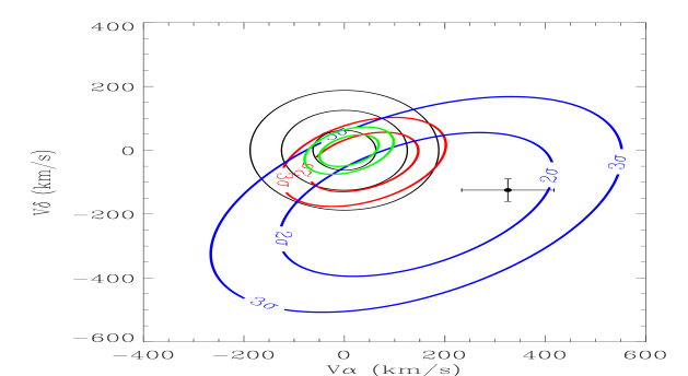
Figure 1: Tangential velocity distributions, $\psi(V_{\alpha},V_{\delta})$, toward the direction ($l=143^{\circ}$, $b=-57^{\circ}$) of WD0135-039 (solid circle). The ellipses show the iso-probability contours (2$\sigma$, 3$\sigma$) of the thin disk, thick disk, and local halo populations based on the kinematic parameters from Binney & Merrifield (1998), Soubiran et al. (2003) and Casertano, Ratnatunga & Bahcall (1990), respectively. The three concentric circles indicate the velocity thresholds, $V_{\rm min}=4.74\mu_{\rm lim}r$, for the OHDHS survey ($\mu_{\rm lim}=0.33^{\prime\prime}$ yr^-1) at the distances $r=40$ pc, 80 pc and 120 pc.

3.3 Thick disk model

The following properties for the population of thick disk WDs in the solar neighborhood were assumed:

• a uniform local space density; for, the typical distance reachable by ground based surveys ($\sim$ 100 pc) is much smaller than the exponential vertical scale-height of the thick disk ($h_{z}\simeq 1000$ pc);

• a velocity distribution (Eq. 1) with ($\sigma_{U},\sigma_{V},\sigma_{W},V_{0})\simeq$ $(63,39,39,-45)$ km s^-1, as derived in Soubiran, Bienaymè & Siebert (2003).

We notice that the velocity ellipsoid of the thick disk population is not currently well established so that this choice will somehow affect the final result. For instance, the presence of a non-gaussian high velocity tail (cfr. Gilmore et al. 2002) would increase the contamination affecting the halo WD sample.

3.4 Kinematically selected samples

In the case of a magnitude- and $\mu$-limited survey with a total extension of $\Omega$ steradians, the following observational constraints need to be taken into account:

1. an apparent magnitude limit $m<m_{\rm lim}$ which implies a distance limit as a function of the absolute magnitude, $M$, of the target:

   $$r<r_{\rm max}(M)=10^{[0.2(m_{\rm lim}-M)+1]}$$

   which, in turn, defines the maximum volume, $V_{\rm Max}(M)=\frac{1}{3}\Omega\,r_{\rm max}^{3}$ covered by the survey;

2. a proper motion limit $\mu>\mu_{\rm lim}$ which translates into a tangential velocity threshold varying with stellar distance:

   $$V_{\rm tan}=\sqrt{V_{\alpha}^{2}+V_{\delta}^{2}}>V_{\rm min}(r)=4.74\mu_{\rm lim}r.$$

Note that, although the distance distribution ($\propto r^{2}$) and the kinematic distribution (Eq. 3 ) of the complete population are independent, now they result correlated for the observed sample because of the existence of the velocity threshold, $V_{\rm min}(r)$.

The probability to select a star with absolute magnitude $M$ in the range $(r,r+dr)$, ($V_{\alpha},V_{\alpha}+dV_{\alpha}$), ($V_{\delta},V_{\delta}+dV_{\delta}$) is then $dP=f(r,V_{\alpha},V_{\delta})drdV_{\alpha}dV_{\delta}$, where the joint probability density is:

$$f(r,V_{\alpha},V_{\delta})=\left\{\begin{array}[]{ll}Kr^{2}\psi(V_{\alpha},V_{\delta})&\mbox{ if }V_{\rm tan}>V_{\rm min}(r)\\ &\mbox{ and }r<r_{\rm max}(M)\\ 0&\mbox{ if }V_{\rm tan}\leq V_{\rm min}(r)\\ &\mbox{ or }r\geq r_{\rm max}(M)\\ \end{array}\right.$$ (4)

Here, $K$ is a normalization constant such that $\int\int\int f\,dr\,dV_{\alpha}\,dV_{\delta}=1$.

If we integrate over $r$ the joint probability density function given in Eq. 4, we obtain the marginal density distribution

$$h(V_{\alpha},V_{\delta}) = \int_{0}^{r_{\rm max}}f(r,V_{\alpha},V_{\delta})\,dr$$ (5)

which quantifies the probability that an object with tangential velocities $(V_{\alpha},V_{\delta})$ could be randomly found somewhere within the whole volume $\frac{1}{3}\Omega\,r_{\rm max}^{3}$, where an object with absolute magnitude $M$ could in principle be observed.

At the same time, we can introduce the (conditional) probability that an object with tangential velocities $(V_{\alpha},V_{\delta})$ is found at the measured distance, $r$:

$$t(V_{\alpha},V_{\delta}|r)=\frac{f(r,V_{\alpha},V_{\delta})}{g(r)}$$ (6)

where

$$g(r)=\int\int_{-\infty}^{+\infty}f(r,V_{\alpha},V_{\delta})\,dV_{\alpha}\,dV_{\delta}$$ (7)

is the marginal density distribution which defines the probability that an object with whatever velocity can be observed at a distance $r$. Because the velocity threshold increases linearly with distance, $V_{\rm min}\propto r$, the space distribution of the proper-motion selected sample (Eq. 7) is also biased towards smaller distances.

Both the marginal distribution $h(V_{\alpha},V_{\delta})$ and the conditional probability $t(V_{\alpha},V_{\delta}|r)$ can be used to test the consistency of each object with a parent population. In principle, the conditional probability $t(V_{\alpha},V_{\delta}|r)$ seems more appropriate than $h(V_{\alpha},V_{\delta})$ since it fully utilizes the individual stellar distances. However, the differences become insignificant when the confidence level is set to sufficiently high values (see next section).

Note that, formally, Eq. 6 is equivalent to the original distribution, $\psi(V_{\alpha},V_{\delta})$, except that the probability is null for $\sqrt{V_{\alpha}^{2}+V_{\delta}^{2}}\leq V_{\rm min}(r)$, and it has been re-normalized.

3.5 Confidence intervals and contamination

Basically, because a proper motion limited survey undersamples the low velocity objects, the main difference between the kinematically selected distributions (Eqs. 5-6) and the complete one (Eq. 3) is that the probability density is redistributed from the low velocity regions towards the high velocity tails. This means that the observed sample is biased towards high velocity objects, as shown for instance by the simulations of Reylé et al. (2001) and Torres et al. (2002).

This effect needs to be taken into account when we define a confidence interval over the $(V_{\alpha},V_{\delta})$ plane in order to test the consistency with the parent population and to estimate the contamination due to objects in the tails beyond the critical limit. In fact, the adoption of the original $\psi(V_{\alpha},V_{\delta})$ to reject the disk stars with respect to a certain confidence level, e.g. $1-\alpha=99\%$, would exclude 99% of all the existing thick disk stars which, however, corresponds to a smaller fraction of the thick disk objects that are really present in the kinematically selected sub-sample. In this case, only the confidence interval defined for $t(V_{\alpha},V_{\delta}|r)$, or $h(V_{\alpha},V_{\delta})$, assures that the fraction of false negatives contaminating the sample of bona fide halo stars does not exceed – on average – 1% of the observed thick disk objects.

In the left panels of Figures 2-3 the concentric ellipses show the iso-probability contours (1$\sigma$, 2$\sigma$, 3$\sigma$) of the velocity distribution expected for thick disk stars, $\psi(V_{\alpha},V_{\delta})$, evaluated in the direction of one of the stars in the Oppenheimer’s sample (LHS 1447), whose tangential velocity is marked with a filled circle. The points represent a Montecarlo realization of 2000 simulated WD’s drawn from the kinematically selected distributions $h(V_{\alpha},V_{\delta})$ and $t(V_{\alpha},V_{\delta}|r)$. The excess of “simulated” thick disk stars with high velocity is evidenced by the fact that there are many more than $\sim$20 objects (1% of the simulated sample) outside the $3\sigma$ confidence interval.

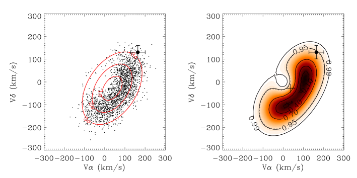
Figure 2: Left panel: iso-probability contours (1$\sigma$, 2$\sigma$, 3$\sigma$) of $\psi(V_{\alpha},V_{\delta})$ compared against a Montecarlo simulation (dots) of the thick disk stars in the direction ($l=226\aas@@fstack{\circ}34$,$b=-64\aas@@fstack{\circ}27$) of LHS 1447 (solid circle) drawn from the kinematically selected distribution, $h(V_{\alpha},V_{\delta})$. Right panel: iso-probability contours (confidence levels of 40%, 70%, 95% and 99%) of $h(V_{\alpha},V_{\delta})$.

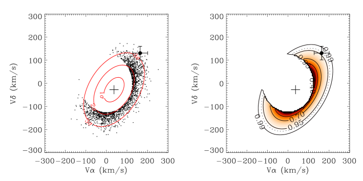
Figure 3: Left panel: iso-probability contours (1$\sigma$, 2$\sigma$, 3$\sigma$) of $\psi(V_{\alpha},V_{\delta})$ compared against a Montecarlo simulation (dots) of the thick disk stars in the direction ($l=226\aas@@fstack{\circ}34$,$b=-64\aas@@fstack{\circ}27$) of LHS 1447 (solid circle) drawn from the kinematically selected distribution, $t(V_{\alpha},V_{\delta}|r)$. Right panel: iso-probability contours (confidence levels of 40%, 70%, 95% and 99%) of $t(V_{\alpha},V_{\delta}|r)$.

LHS 1447 is also located outside the 3$\sigma$ contour so that, according to the complete distribution, it should be rejected as a thick disk star with a confidence level higher than $1-\alpha=$99%. Actually, that conclusion would be incorrect if we tested the hypothesis that LHS 1447 is a member of the kinematically selected sample as shown in the right panels of Figures 2-3, where the marginal and conditional distributions, $h(V_{\alpha},V_{\delta})$ and $t(V_{\alpha},V_{\delta}|r)$, are drawn. In fact, in these cases the star is located within the iso-probability contour delimiting the 99% confidence level so that it must be accepted as a thick disk star.

4 Results and discussion

Both distributions, $h(V_{\alpha},V_{\delta})$ and $t(V_{\alpha},V_{\delta}|r)$, were used to analyze the WD sample in the OHDHS survey.

The kinematic tests were carried out in the tangential plane of each individual star so that no assumption on radial velocity is necessary. The values of 95% and 99% for the confidence level ($1-\alpha$) were chosen in order to minimize the presence of false negatives. With a total sample of 98 WDs, presumably a mixture of (thin and thick) disk and halo WDs, we expect that $<1$ (99%) and $<5$ (95%) of the high velocity thick disk stars would contaminate the selected Pop. II WD sample.

Table 1: Estimation of the halo WD density based on the objects selected from the OHDHS sample.

Confid.	$\psi(V_{\alpha},V_{\delta})$		$h(V_{\alpha},V_{\delta})$		$t(V_{\alpha},V_{\delta}|r)$
level	WDs	$\rho_{\rm WD}$ (M⊙pc-3)	WDs	$\rho_{\rm WD}$ (M⊙pc-3)	WDs	$\rho_{WD}$ (M⊙pc-3)
99%	14	$(2.0\pm 0.9)\cdot 10^{-5}$	10	$(1.6\pm 0.8)\cdot 10^{-5}$	10	$(1.5\pm 0.8)\cdot 10^{-5}$
95%	20	$(3.1\pm 1.0)\cdot 10^{-5}$	12	$(1.9\pm 0.9)\cdot 10^{-5}$	13	$(2.0\pm 0.9)\cdot 10^{-5}$

Table 2: Estimation of the halo WD density based on the sample revised by Salim et al. (2004).

Confid.	$\psi(V_{\alpha},V_{\delta})$		$h(V_{\alpha},V_{\delta})$		$t(V_{\alpha},V_{\delta}|r)$
level	WDs	$\rho_{\rm WD}$ (M⊙pc-3)	WDs	$\rho_{\rm WD}$ (M⊙pc-3)	WDs	$\rho_{\rm WD}$ (M⊙pc-3)
99%	19	$(1.8\pm 0.6)\cdot 10^{-5}$	17	$(1.6\pm 0.6)\cdot 10^{-5}$	16	$(1.5\pm 0.6)\cdot 10^{-5}$
95%	28	$(3.3\pm 0.8)\cdot 10^{-5}$	18	$(1.8\pm 0.6)\cdot 10^{-5}$	18	$(1.9\pm 0.6)\cdot 10^{-5}$

4.1 Halo WD density

In Table 1 we report the results based on this procedure for the WD sample published by OHDHS. We only found 10 objects which do not appear consistent with the kinematically selected density distributions, $h(V_{\alpha},V_{\delta})$ and $t(V_{\alpha},V_{\delta}|r)$, at the 99% confidence level, while 12-13 probable halo WDs are selected when $1-\alpha=95$%. As expected, the number of candidates increases up to 14 (99%) or 20 (95%) in the case of a test based on the complete distribution, $\psi(V_{\alpha},V_{\delta})$, mainly because of a higher contamination.

Finally, the halo WD density was estimated by means of the classical 1/V_Max method (Schmidt 1975), and assuming a value of 0.6 M_⊙ for the typical WD mass. The results, with their (poissonian only) errors, are reported in Tab. 1, where the different values refer to the two confidence levels and the three probability distributions used for the calculations.

Although affected by large uncertainties, the values in Tab. 1 suggest a density of $\rho_{\rm WD}\approx$ $10^{-5}$ M_⊙pc^-3, i.e. 0.1-0.2% of the local dark matter, which is an order of magnitude smaller than what reported in OHDHS.

Our results are consistent with the local mass density of halo WDs estimated by Gould et al. (1998), and with various reanalyses of the OHDHS sample (e.g. Reid et al. 2001, Reylé et al. 2001, Torres et al. 2002, Salim et al. 2004). Furthermore, Carollo et al. (2004), applying the statistical methodology described in this paper on a new high proper motion survey based on GSC-II material, derived a similar value of $\sim 10^{-5}$ M_⊙pc^-3.

Lacking individual trigonometric parallaxes, a critical point of this (and any) analysis is the choice of the method for the estimation of the distances, which directly affects the evaluation of the WD tangential velocities and, of course, of their stellar density. As remarked by several authors (see e.g. Torres et al. 2002, Bergeron 2003), empirical and theoretical CM relations can both give rise to systematic errors.

To this regard, if for the distances of the OHDHS sample we adopt the values recently redetermined by Salim et al. (2004), the number of selected halo WDs increases but the resulting densities, shown in Table 2, are not significantly different from those reported in Table 1.

4.2 Distance and velocity errors

The large error, $\sim$ 20-30%, affecting WD photometric parallaxes, cannot be neglected in a rigorous statistical analysis. Basically, besides the contribution of the photometric errors, the large uncertainty in the distance modulus, $m-M$, derives from the large intrinsic dispersion ($\sigma_{\rm Mv}\simeq 0.4$ - 0.5 mag) of the CM relation, a consequence of the superposition of cooling sequences of WDs of different masses and atmospheres.

Table 3: Same as Tab.1 after adopting a thick disk velocity distribution convolved with the observation errors.

Confid.	$\psi(V_{\alpha},V_{\delta})$		$h(V_{\alpha},V_{\delta})$		$t(V_{\alpha},V_{\delta}|r)$
level	WDs	$\rho_{\rm WD}$ (M⊙pc-3)	WDs	$\rho_{\rm WD}$ (M⊙pc-3)	WDs	$\rho_{\rm WD}$ (M⊙pc-3)
99%	6	$(1.3\pm 0.8)\cdot 10^{-5}$	3	$(1.2\pm 0.8)\cdot 10^{-5}$	3	$(1.2\pm 0.8)\cdot 10^{-5}$
95%	14	$(2.0\pm 0.9)\cdot 10^{-5}$	5	$(1.3\pm 0.8)\cdot 10^{-5}$	6	$(1.3\pm 0.8)\cdot 10^{-5}$

Table 4: Same as Tab.2 after adopting a thick disk velocity distribution convolved with the observation errors.

Confid.	$\psi(V_{\alpha},V_{\delta})$		$h(V_{\alpha},V_{\delta})$		$t(V_{\alpha},V_{\delta}|r)$
level	WDs	$\rho_{\rm WD}$ (M⊙pc-3)	WDs	$\rho_{\rm WD}$ (M⊙pc-3)	WDs	$\rho_{\rm WD}$ (M⊙pc-3)
99%	14	$(1.2\pm 0.5)\cdot 10^{-5}$	8	$(0.7\pm 0.4)\cdot 10^{-5}$	5	$(0.6\pm 0.4)\cdot 10^{-5}$
95%	18	$(1.7\pm 0.6)\cdot 10^{-5}$	14	$(1.2\pm 0.5)\cdot 10^{-5}$	9	$(1.0\pm 0.5)\cdot 10^{-5}$

In practice, the main effect of the tangential velocity errors, $\epsilon_{V}/V=\sqrt{(\sigma_{\mu}/\mu)^{2}+(\sigma_{d}/d)^{2}}$, is to increase the dispersion and the overlap of the “observed” kinematic distributions belonging to the various stellar populations. Clearly this also increases the contamination of the disk WDs and makes the identification of the halo WDs more difficult.

Although a more rigorous statistical analysis should be necessary to consider properly the presence of these errors, a conservative estimation can be given by selecting only those objects which are not consistent with the “observed” kinematic distribution that results from convolving the projected kinematic distribution of the thick disk (Eq. 3) with a bivariate gaussian error distribution with null mean and dispersions, ($\epsilon_{V\alpha},\epsilon_{V\delta})_{(i)}$, corresponding to the velocity errors of the $i$-th object. The velocity errors have been derived by assuming the proper motion errors, $\sigma_{\mu}$, listed in Tab. 1 of OHDHS, and a more realistic photometric parallax error, $\sigma_{d}/d$, of 25% (instead of 20%).

The different halo WD densities estimated from the objects which are not consistent (at the 95% and 99% confidence level) with the new distributions are reported in Tables 3 and 4. Because of the larger velocity thresholds, the number of selected halo WDs is smaller than those reported in Tables 1 and 2. The estimated WD densities, uncorrected for the loss of halo WDs with disk kinematics, decrease proportionally, but are still consistent with $\rho_{\rm WD}\sim 10^{-5}$ M_⊙pc^-3. Note that the minimum values, which are reported in Tab. 4, have been derived from the data of Salim et al. (2004) who provided distances (and thus volumes) systematically larger than OHDHS.

4.3 On the thick disk model

As mentioned in Sect. 3.3, our selection criterion depends implicitly also on the choice of the kinematic parameters adopted for the thick disk, whose spatial and kinematical properties are still matter of debate and investigation. Here, we have used the velocity ellipsoid recently derived by Soubiran et al. (2003) from a sample of $\sim$ 400 giants with 3D kinematics at a distance of 200-800 pc towards the North Galactic Cap. Their results are very close to the kinematic parameters estimated by Casertano, Ratnatunga & Bahcall (1990) and are consistent with various other determinations of the thick disk kinematics, which support velocity dispersions of 40-60 km s^-1 and an asymmetric drift in the range 30-50 km s^-1.

Although controversial, some authors claim the presence of a vertical velocity gradient, that supports a thick disk which rotates faster close to the galactic plane (i.e. where the WD sample is localized), than at higher Z’s, where the studies of the thick disk kinematics have been usually carried out. In particular, Chiba & Beers (2000), who analyzed 1203 metal poor stars non-kinematically selected, found a rapidly rotating thick disk close to the galactic plane with a small asymmetric drift $V_{0}\simeq-20$ km s^-1 and with velocity dispersions ($\sigma_{U},\sigma_{V},\sigma_{W})\simeq$ $(46\pm 4,50\pm 4,35\pm 3)$ km s^-1. Moreover, they determined a velocity gradient $\partial V_{0}/\partial|Z|\simeq-30\pm 3$ km s^-1 kpc^-1, that, however, other studies (e.g. Soubiran et al. 2003) do not detect. Nevertheless, a fast rotating thick disk at $Z\approx 0$ was determined also by Upgren et al. (1997) from a sample of K-M dwarfs in the solar neighborhood ($d\la 50$ pc) with trigonometric parallaxes and proper motions from the Hipparcos catalogue and radial velocity measurements.

Thus, in order to test the sensitivity of our method with respect to the adopted thick disk model, we repeated the WD selection of the Salim et al. (2003) sample through the distributions $h(V_{\alpha},V_{\delta})$ and $t(V_{\alpha},V_{\delta}|r)$ derived using the velocity ellipsoid from Chiba & Beers (2000). The new results are consistent (within 1$\sigma$) with the values obtained with the kinematics from Soubiran et al. (2003), although the resulting densities appear typically larger than the previous ones.

For instance, with a 99% confidence level we find $\rho_{\rm WD}\simeq(1.7\pm 0.6)10^{-5}$ M_⊙pc^-3 for both $h(V_{\alpha},V_{\delta})$ and $t(V_{\alpha},V_{\delta}|r)$ when the velocity errors are not taken into account (cfr. Tab. 2), while the distributions convolved with the velocity errors provide $\rho_{\rm WD}\simeq(0.9\pm 0.5)10^{-5}$ M_⊙pc^-3 (cfr. Tab. 4). The 95% confidence level also provides similar but systematically higher new densities up to $(1.8\pm 0.7)10^{-5}$ M_⊙pc^-3 and $(3.0\pm 0.9)10^{-5}$ M_⊙pc^-3 respectively when the velocity errors are, or are not, convolved with the tangential velocity distributions.

Anyhow, it appears that, with the adopted confidence levels, significantly higher density (e.g. close to $\sim 10^{-4}$ M_⊙pc^-3 may be attained only with disk ellipsoids kinematically much “cooler” than those expected for a typical thick disk population. For instance, a total density $(8.8\pm 0.2)10^{-5}$ M_⊙pc^-3 is only obtained counting all the 41 WDs which are not consistent with the thin disk kinematics (using $t(V_{\alpha},V_{\delta}|r)$ with a 95% confidence level), i.e. summing both halo and thick disk WDs.

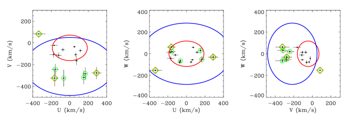
Figure 4: Velocity distribution (U,V,W) of the subsample of 15 stars with available radial velocity (dots with 1$\sigma$ error bars) from Salim et al. (2004). The objects selected by means of the distributions $h(V_{\alpha},V_{\delta})$ and $t(V_{\alpha},V_{\delta}|r)$ with a 95% confidence level (Tab. 4) are marked with circle and diamond symbols, respectively. The ellipses show the $3\sigma$ iso-probability contours of the thick disk and halo velocity distribution.

4.4 UVW distribution

Salim et al. (2003) provide radial velocities for 15 DA WDs, 13 of which derived from new measurements of the OHDHS sample and two from Pauli et al. (2003), so that, in principle, a more accurate kinematic membership for these objects may be inferred using the information from the full 3D velocities. This requires 3D velocity distributions for kinematically selected samples which are beyond the scope of the current study. However, the availability of both tangential and radial velocities for this subsample offers the possibility to check a posteriori the efficiency of the 2D kinematic analysis adopted in this work and described in Sect. 3.

To this regard, Figure 2 shows the (U,V,W) velocities derived from Eq. 2 for the 15 stars with available radial velocity. Those which have been selected with a 95% confidence level by means of the distributions $h(V_{\alpha},V_{\delta})$ and $t(V_{\alpha},V_{\delta}|r)$ convolved with the velocity errors (Tab. 4) are marked with square and diamond symbols. In addition, the $3\sigma$ iso-probability ellipses of the thick disk and halo velocity distributions, based on the kinematic parameters respectively from Soubiran et al. (2003) and Casertano, Ratnatunga & Bahcall (1990), are also plotted. The three panels of Fig. 2 indicate that, basically, all the likely halo WDs have been properly identified by our kinematic analysis based on the 2D $(V_{\alpha},V_{\delta})$ distributions, thus supporting the reliability of our selection procedure.

5 Conclusions

A kinematically selected sample made of 98 WDs with $\mu>$ 0.33$\arcsec yr^{-1}$ was published by OHDHS who performed a high proper motion survey over 4165 deg² toward the SGP down to $R59F\simeq 19.8$. These data stimulated a number of studies addressing the issue that a significant part of the dark halo of the Milky Way could be composed of matter in the form of ancient cool WDs. The basic problem – as addressed by several authors – is the criterion to disentangle the mixture of (thick) disk and halo objects on the basis of their kinematic properties and ages.

To this regard, we have implemented a general method for the kinematic analysis of high proper motion surveys and applied it to the identification of reliable halo stars. The kinematically-selected tangential velocity distributions are derived for every star, so that no assumption on the unknown third velocity component, $V_{r}$, nor any approximation on the galactic components (U,V,W), is necessary.

We selected as bona fide halo WDs only those stars whose tangential velocity is inconsistent, at the 95% and 99% confidence levels, with the appropriate projected distribution, $h(V_{\alpha},V_{\delta})$ or $t(V_{\alpha},V_{\delta}|r)$, of the observed thick disk population, thus assuring limited contamination of thick disk objects. Finally, the effect of large velocity errors, which derive from the intrinsic uncertainty of the WD photometric parallaxes, was also discussed and taken into account.

We applied this methodology to the OHDHS sample and selected 10 probable halo WDs (that became 3 after the inclusion of the velocity errors) at the a 99% confidence level. Through the 1/V_Max method, we estimated a local WD density of $\rho_{\rm WD}\simeq 1\div 2\cdot 10^{-5}$ M_⊙pc^-3 (i.e. 0.1-0.2% of the local dark matter) which is consistent with the values found by Gould et al. (1998), as well as by other authors who reanalyzed the OHDHS sample (e.g. Reid et al. 2001, Reylé et al. 2001, Torres et al. 2002, Flynn et al. 2003). The same methodology applied to the OHDHS sample revised by Salim et al. (2004) yields a similar value. These results agree with those found by Carollo et al. (2004) from a first analysis of new data of an independent high proper motion survey in the Northern hemisphere based on material and procedures used for the construction of the GSC-II.

Although affected by a large uncertainty due to the small statistics and low accuracy of the photometric parallaxes, our results clearly indicate that ancient cool WDs do not contribute significantly to the baryonic fraction of the galactic dark halo, as possibly suggested by the microlensing experiments which claimed that $\sim$ 20% of the dark matter is formed by compact objects of $\sim$ 0.5 M_⊙ (Alcock et al. 2000).

- (1) Alcock C. et al. 2000, ApJ, 542, 281
- (2) Bergeron, P. 2003, ApJ, 586, 201
- (3) Bergeron, P., Ruiz, M.T., & Leggett, S.K. 1997, ApJS, 108, 339
- (4) Bergeron, P., Leggett, S. K., & Ruiz, M.T. 2001, ApJS, 133, 413
- (5) Binney, J. & Merrifield, M. 1998, Galactic Astronomy, Princeton Univ. Press
- (6) Carollo, D. et al. 2004, XXVth IAU General Assembly, JD 5, Sidney (Australia), Jul 16-17, Shipman H. & Sion E.M. eds., in press
- (7) Casertano, S. et al. 1990, ApJ, 357, 435
- (8) Chiba, M. & Beers T.C. 2000, ApJ, 119, 2843
- (9) Dehnen, W. & Binney, J.J. 1998, MNRAS, 298, 387
- (10) Flynn C. et al., 2003, MNRAS, 339, 817
- (11) Gilmore, G. et al., 2002, ApJ, 574L, 39
- (12) Gould, A. et al. 1998, ApJ, 503, 798
- (13) Hambly, N. C. et al., 2001, MNRAS, 326, 1279
- (14) Hansen, B.M.S. 2001, ApJ, 558L, 39
- (15) Hansen, B.M.S. & Liebert, J. 2003, ARA&A, 41, 465
- (16) Koopmans, L.V.E., & Blandford, R.D. 2002, MNRAS, submitted (astro-ph/0107358)
- (17) Nelson, C.A., Cook, K.H., Axelrod, T.S., Mould, J.R. & Alcock, C. 2002, ApJ, 573, 644
- (18) Oppenheimer, B.R., Hambly, N.C., Digby, A.P., Hodgkin, S.T. & Saumon, D. 2001, Science, 292, 698 (OHDHS)
- (19) Pauli, E.M., Napiwotzki, R., Altmann, M., Heber, U., Odenkirchen, M., & Kerber, F. 2003, A&A, 400, 877
- (20) Reid, I.N., Sahu K.C., & Hawley S.L. 2001, ApJ, 559, 942
- (21) Reylé, C., Robin, A.C., & Creze, M. 2001, A&A, L53
- (22) Salim, S., Rich, R.Mi., Hansen, B.M., Koopmans, L.V.E., Oppenheimer, B.R. & Blandford, R.D. 2004, ApJ, 601, 1075
- (23) Schmidt, M. 1975, ApJ, 202, 22
- (24) Soubiran, C. et al. 2003, A&A, 398, 141
- (25) Torres, S., García-Berro, E., Burkert, A., & Isern, J. 2002, MNRAS, 336, 971
- (26) Trumpler R.J. & Weaver H.F., 1953, Statistical Astronomy, Univ. of California press
- (27) Upgren, A.R., Ratnatunga, K.U., Casertano, S. & Weis, E. 1997, Proc. of the ESA Symposium Hipparcos - Venice 97, 13-16 May, 1997, Venice (I), ESA SP-402, 583