Physical Properties and Baryonic Content of Low-Redshift Intergalactic Ly$\alpha$ and O VI Absorption Line Systems: The PG 1116+215 Sight Line ^,

Abstract

We present Hubble Space Telescope and Far Ultraviolet Spectroscopic Explorer observations of the intergalactic absorption toward QSO PG 1116+215 in the $900-3000$ Å spectral region. We detect 25 Ly$\alpha$ absorbers along the sight line at rest-frame equivalent widths $W_{r}>30$ mÅ, yielding (d$N$/d$z$)${}_{{\rm Ly}\alpha}=154\pm 18$ over an unblocked redshift path $\Delta X_{{\rm Ly}\alpha}=0.162$. Two additional weak Ly$\alpha$ absorbers with $W_{r}\approx 15-20$ mÅ are also present. Eight of the Ly$\alpha$ absorbers have large line widths (b $\gtrsim 40$  km s^-1). The detection of narrow O VI absorption in the broad Ly$\alpha$ absorber at $z=0.06244$ supports the idea that the Ly$\alpha$ profile is thermally broadened in gas with $T>10^{5}$ K. We find d$N$/d$z$ $\approx 50$ for broad Ly$\alpha$ absorbers with $W_{r}\gtrsim 30$ mÅ and ${\rm b}\geq 40$  km s^-1. This number drops to d$N$/d$z$ $\approx 37$ if the line widths are restricted to $40\leq{\rm b}\leq 100$  km s^-1. If the broad Ly$\alpha$ lines are dominated by thermal broadening in hot gas, the amount of baryonic material in these absorbers is enormous, perhaps as much as half the baryonic mass in the low-redshift universe. We detect O VI absorption in several of the Ly$\alpha$ clouds along the sight line. Two detections at $z=0.13847$ and $z=0.16548$ are confirmed by the presence of other ions at these redshifts (e.g., C II-III, N II-III, N V, O I, and Si II-IV), while the detections at $z=0.04125$, $0.05895$, $0.05928$, and $0.06244$ are based upon the Ly$\alpha$ and O VI detections alone. We find (d$N$/d$z$)${}_{\rm O\,VI}\approx 17$ for O VI absorbers with $W_{r}>50$ mÅ toward PG 1116+215. The information available for 13 low-redshift O VI absorbers with $W_{r}\geq 50$ mÅ along 5 sight lines yields (d$N$/d$z$)${}_{\rm O\,VI}\approx 14$ and $\Omega_{b}$(O VI) $\gtrsim 0.0027h_{75}^{-1}$, assuming a metallicity of 0.1 solar and an O VI ionization fraction $f_{\rm O\,VI}\leq 0.2$. The properties and prevalence of low-redshift O VI absorbers suggest that they too may be a substantial baryon repository, perhaps containing as much mass as stars and gas inside galaxies. The redshifts of the O VI absorbers are highly correlated with the redshifts of galaxies along the sight line, though few of the absorbers lie closer than $\sim 600\,h_{75}^{-1}$ kpc to any single galaxy. We analyze the kinematics and ionization of the metal-line systems along this sight line and discuss the implications of these observations for understanding the physical conditions and baryonic content of intergalactic matter in the low-redshift universe.

1 Introduction

There is strong evidence that the warm-hot (T $\sim 10^{5}-10^{7}$ K) intergalactic medium (IGM) is a significant repository of baryons in the low-redshift universe. The observational basis for this assertion is the growing sample of absorption-line systems found to contain highly ionized stages of oxygen (e.g., O VI – Tripp, Savage, & Jenkins 2000; Tripp & Savage 2000; Savage et al. 2002) and/or broad H I Ly$\alpha$ absorption (Richter et al. 2004). These measurements, which are being made with the spectrographs on the Hubble Space Telescope (HST) and Far Ultraviolet Spectroscopic Explorer (FUSE), are available for only a small number of sight lines, but they already indicate that the hot gas may be prevalent throughout the nearby universe. In addition, X-ray detections of higher ionization species (e.g., O VII) at X-ray wavelengths with the Chandra X-ray Observatory and XMM-Newton point to a large amount of coronal gas in the Local Group if the absorption does not arise within the interstellar medium of the Galaxy along the lines of sight surveyed (e.g., Nicastro et al. 2002; Fang, Sembach, & Canizares 2003; Rasmussen, Kahn, & Paerels 2003). Support for an extended distribution of coronal gas around the Milky Way is bolstered by detections of O VI absorption at the boundaries of high-velocity clouds located at large distances from the Galactic plane (Sembach et al. 2000; 2003).

The low-redshift O VI and Ly$\alpha$ observations favor the presence of warm-hot ($10^{5}-10^{7}$ K) intergalactic gas predicted by theoretical and numerical expectations for the evolution of intergalactic gas in the presence of cold dark matter (e.g., Cen & Ostriker 1999a; Davé et al. 1999, 2001). Hydrodynamical simulations of the cosmos predict that Ly$\alpha$ clouds evolve to form extended filamentary and sheet-like structures. These sheets and filaments gradually collapse into denser concentrations and form galaxies. As this happens, shocks heat the gas to high temperatures. The gas density, temperature, and metallicity of the warm-hot IGM depend upon the evolutionary state of the gas and its proximity to galaxies (Cen & Ostriker 1999b), so it is important to obtain spectroscopic observations of O VI and other absorption lines to gain insight into the physical conditions and environments of the absorbers detected.

An initial census of low-redshift O VI absorbers along 5 sight lines observed with the HST and FUSE indicates that the number of O VI absorbers per unit redshift is (d$N$/d$z$)${}_{\rm OVI}\approx 14\pm^{9}_{6}$ (Savage et al. 2002 and references therein). Assuming a metallicity of 0.1 solar and converting this number density to a mass implies a cosmic baryon density $\Omega_{b}$(O VI) $\gtrsim 0.002h^{-1}_{75}$ in these O VI absorbers, which is comparable to the baryonic mass in galaxies (Fukugita, Hogan, & Peebles 1998). This estimate depends critically on knowing the metallicity and ionization properties of the O VI systems since the total gas column must be calculated from the observed O VI column densities (i.e., N_H = N(O VI) $\times$ N(O)/N(O VI) $\times\,{\rm(O/H)}^{-1}$). Determining the total baryonic content of the O VI absorbers therefore requires estimates of the amount of gas in the different types of systems in which O VI is found (photoionized, collisionally ionized, mixed ionization, etc). This is particularly important in light of recent estimates for the amount of gas that may be contained in broad Ly$\alpha$ absorbers (Richter et al. 2004; see also §9.2). Some of the broad Ly$\alpha$ absorbers contain detectable amounts of O VI, and some do not (see §9.2).

Distinguishing between different types of O VI systems and quantifying N(O)/N(O VI) and the gas metallicity are best accomplished by comparing the O VI absorption to absorption by other species detected at ultraviolet and X-ray wavelengths. High resolution ultraviolet spectroscopy permits detailed kinematical comparisons of the high ionization lines (e.g., O VI) with lower ionization metal-line species (e.g.,C II-III-IV, Si III-IV, Al III) and H I Lyman-series features. Close kinematical coupling of O VI with lower ionization stages would suggest that the warm-hot and cool IGM are mixed or in close proximity. X-ray measurements may also hold great promise for placing gas hotter than that traced by O VI (e.g., $T>10^{6}$ K) in context, but current X-ray instruments provide only low-resolution ($\lambda/\Delta\lambda<750$) measurements of bulk kinematics and column densities in absorption toward only the very brightest AGNs/QSOs (see, e.g., Mathur, Weinberg, & Chen 2003).

To date, only a handful of sight lines of been surveyed for low-redshift O VI absorption and broad H I Ly$\alpha$ absorption. Even fewer have had systematic galaxy survey information published to assess the relationship of the absorbers and galaxies. In this paper we discuss the physical properties and baryonic content of the Ly$\alpha$ and O VI absorption line systems along the PG 1116+215 sight line. Section 2 contains a description of the observations and data reduction. In §3 we briefly describe the sight line and the Galactic foreground absorption. We also calculate the unblocked redshift paths available to search for Ly$\alpha$ and O VI absorption. In §4 we provide information about the identification of the absorption lines in the FUSE and STIS spectra. Section 5 contains a brief overview of each intergalactic absorption line system identified. Sections 6 and 7 contain detailed information for the two metal-line systems at $z=0.13847$ and $z\approx 0.166$. Section 8 summarizes the information for several additional weak O VI absorbers detected. Section 9 describes the properties of the Ly$\alpha$ systems along the sight line and includes an estimate for the baryonic mass in the broad Ly$\alpha$ absorbers. In §10 we examine the relationship between the absorption systems and nearby galaxies. We conclude in §11 with a discussion of the baryonic content of the warm-hot intergalactic medium. Section 12 contains a summary of the primary results of the study.

2 Observations and Data Reduction

The spectral range covered by the FUSE and HST/STIS data obtained for this study is shown in Figure 1, where we have binned the spectra into 0.2 Å wide bins for clarity. All measurements and line analyses in this paper were conducted on optimally sampled data. Unless otherwise state, all velocities in this paper are given in the heliocentric reference frame. Note that in the direction of PG 1116+215 the Local Standard of Rest (LSR) and heliocentric reference frames are nearly identical: $v_{\rm LSR}=v_{\rm helio}+1$  km s^-1.

2.1 Far Ultraviolet Spectroscopic Explorer Observations

We observed PG 1116+215 with FUSE in April 2000 and April 2001 as part of the FUSE Team low-redshift O VI project. For all observations PG 1116+215 was aligned in the center of the LiF1 channel LWRS ($30\arcsec\times 30\arcsec$) aperture used for guiding. The remaining channels were co-aligned throughout the observations. The initial observation in April 2000 consisted of 7 exposures totaling 11 ksec of exposure time. The second set of observations in April 2001 consisted of 36 exposures totaling 66 ksec in the LiF channels and 53 ksec in the SiC channels after screening the time-tagged photon-address lists for valid data. Table 1 contains a summary of the FUSE observations of PG 1116+215.

We processed the FUSE data with a customized version of the standard FUSE pipeline software (CALFUSE v2.2.2). This processing followed the detailed calibration steps used in previous FUSE investigations by our group (e.g., Sembach et al. 2001, 2004; Savage et al. 2002). An overview of FUSE and the general calibration measures employed can be found in Moos et al. (2000) and Sahnow et al. (2000). For each channel (LiF1, LiF2, SiC1, SiC2), we made a composite spectrum that incorporated all of the available data for the channel. The FUSE observations span the 905–1187 Å spectral region, with at least two channels covering any given wavelength over most of this wavelength range.

We registered the composite spectra for the four channels to a common heliocentric reference frame by aligning the velocities of Galactic interstellar features with similar absorption lines in the HST/STIS band (e.g., C II $\lambda 1036.337$ vs.  $\lambda 11334.532$; Si II $\lambda 1020.699$ vs. $\lambda 1304.370$; Fe II $\lambda 1144.938$ vs. $\lambda 1608.451$). We also made cross-element comparisons (e.g., Si II $\lambda 1020.699$ vs. S II $\lambda\lambda 1250.584,1253.811$, etc.). For all such comparisons, we considered only the low velocity portions of the interstellar profiles so as not to bias the velocity comparisons made as part of a companion study of the high-velocity Galactic absorption along the sight line (Ganguly et al. 2004). The fully processed and calibrated FUSE spectra have a nominal zero-point velocity uncertainty of $\sim 5$  km s^-1 ($1\sigma$). The relative velocity uncertainties across the bandpass are comparable in size to this zero-point uncertainty but can be larger near the edges of the detectors.

We binned the oversampled FUSE spectra to a spectral bin size of 4 pixels, or $\sim 0.025$ Å ($\sim 7.5$  km s^-1). This binning provides approximately 3 samples per spectral resolution element of 20–25  km s^-1 (FWHM). The data have continuum signal-to-noise ratios $S/N\sim 18$ and 14 per spectral resolution element in the LiF1 and LiF2 channels at 1050 Å, and $S/N\sim 8$ and 13 at 950 Å in the SiC1 and SiC2 channels, respectively.

We show the FUSE data in Figure 2, where we plot the composite spectra in the SiC1 and SiC2 channels below $\sim 1000$ Å, and the composite LiF1 and LiF2 spectra above $\sim 1000$ Å, as a function of heliocentric wavelength. Between $\sim 1075$ and $\sim 1090$ Å, SiC data are used to cover the wavelength gaps in the LiF coverage caused by the physical gaps between detector segments. Line identifications for those features marked above the spectra are listed to the right of each panel. Redshifts are indicated in parentheses for intergalactic absorption features. Rest wavelengths (in Å) are provided for Galactic lines ($\lambda>912$ Å: Morton 1991, 2003; $\lambda<912$ Å: Verner et al. 1994). Numerous molecular hydrogen (H₂) lines in the spectrum are indicated by their rotational band and level (L = Lyman band, W = Werner band) and vibrational level according to standard transition selection rule notations. The wavelengths of the molecular hydrogen lines are from Abgrall et al. (1993a, 1993b). For some Galactic lines, a high-velocity feature is also present (Ganguly et al. 2004); these features are indicated with offset tick marks connected to the corresponding zero-velocity tick marks above the spectra.

The fully calibrated FUSE data have a slightly higher flux than the STIS data in regions where the spectra overlap [$1160\lesssim\lambda{\rm(\AA)}\lesssim 1190$]. The difference in the continuum levels is approximately 30% (see Figure 1). The flux level differences, which may be due to intrinsic variability in the QSO continuum levels in the 11 months separating the FUSE and STIS observations, do not affect any of the analyses or results in this paper.

2.2 Space Telescope Imaging Spectrograph Observations

We observed PG 1116+215 with HST/STIS in May 2000 and June 2000 as part of Guest Observer programs GO-8097 and GO-8165. We used the E140M grating with the $0.2\arcsec\times 0.06\arcsec$ slit for our primary observations. The May 2000 E140M observations consist of 14 exposures totaling 19.9 ksec, and the June 2000 observations consist of 14 exposures totaling 20 ksec. We also obtained a set of E230M exposures (3 exposures, 5.6 ksec total) as part of program GO-8097. Table 2 contains a summary of the STIS E140M and E230M observations of PG 1116+215.

We followed the standard data reduction and calibration procedures used in our previous STIS investigations (see Savage et al. 2002; Tripp et al. 2001; Sembach et al. 2004). We combined the individual exposures with an inverse variance weighting and merged the echelle orders into a composite spectrum after calibrating and extracting each order. We used the two-dimensional scattered light subtraction algorithm developed by the STIS Instrument Definition Team (Landsman & Bowers 1997; Bowers et al. 1998). The STIS data have a zero-point heliocentric velocity uncertainty of $\approx 1$  km s^-1 and a spectral resolution of 6.5  km s^-1 (FWHM).   The spectra have $S/N\approx 15$ per resolution element at 1300 Å. Details on the design and performance of STIS can be found in articles by Woodgate et al. (1998) and Kimble et al. (1998). For additional information about observations made with STIS, we refer the reader to the STIS Instrument Handbook (Proffitt et al. 2002).

We plot the STIS E140M data in Figure 3 as a function of heliocentric wavelength between 1167 Å  and 1649 Å in a manner analogous to the presentation for the FUSE data in Figure 2. The data shown in Figure 3 span E140M echelle orders 90–126. The full STIS spectrum extends from 1144 Å to 1709 Å. At $\lambda<1170$ Å, $S/N\lesssim 4$ per resolution element.

Figure 4 contains selected regions of our STIS E230M observation of PG 1116+215. The spectrum spans echelle orders 73–101 and covers the 2004–2818 Å wavelength range. The spectrum is very noisy at $\lambda<2200$ Å and has $S/N\approx 10-12$ per 10  km s^-1 resolution element between 2400 Å and 2800 Å. All of the lines detected are Galactic in origin, but the data allow us to set upper limits on the presence of some metal-line species in the $z=0.13847$ absorber along the sight line.

For comparison with previous low-resolution HST/GHRS observations of PG 1116+215 (Tripp et al. 1998), we show the full-resolution STIS spectrum in Figure 5 together with the STIS E140M spectrum convolved to the GHRS G140L resolution of $\sim 160$  km s^-1 (FWHM). Nearly all of the features detected in the earlier high-$S/N$ GHRS spectrum appear in the convolved STIS E140M spectrum as well. Most of these features are composed of multiple absorption lines, as revealed in the full spectral resolution plots shown in Figure 3 and the bottom panel of Figure 5.

3 The PG 1116+215 Sight Line

PG 1116+215 lies in the direction $l=223\fdg 36,b=+68\fdg 21$ at a redshift $z_{em}=0.1763\pm 0.0008$, as measured from the Ly$\alpha$ emission in our STIS spectrum. This redshift is similar to the value of $z_{em}=0.1765\pm 0.0004$ found by Marziani et al. (1996). The sight line extends through the Galactic disk and halo, several high-velocity clouds located in or near the Galaxy, and the intergalactic medium. Absorption lines arising in gas in all of these regions are present in the spectra shown in Figures 2–4. Table 3 contains the wavelengths and oscillator strengths ($f$-values) for the interstellar features with observed wavelengths greater than 917 Å identified in Figures 2 and 3. Most of these lines are cleanly resolved from nearby lines in the STIS band and the FUSE band above 1000 Å. Below 1000 Å, line crowding becomes more problematic, especially at wavelengths less than 940 Å, where numerous H I Lyman-series and O I lines are present. The interstellar lines generally consist of two main absorption components centered near $v_{\rm LSR}=-44$  km s^-1 and 0  km s^-1, with additional weaker components occurring between –100 and +100  km s^-1. The total H I column density along the sight line measured through H I 21 cm emission is N(H I) = $1.2\times 10^{20}$ cm^-2, with about 60% of the H I in the stronger complex near –44  km s^-1 (see Wakker et al. 2003). Molecular hydrogen in the $J=0-3$ rotational levels is present in the –44  km s^-1 absorption complex; see Richter et al. (2003) for a detailed study of the molecular lines in the PG 1116+215 spectra. The high-velocity gas, which is detected in a wide range of ionization stages, is centered near +184  km s^-1, with some lines (e.g., C III $\lambda 977.020$, C IV $\lambda\lambda 1548.195,1550.770$, O VI $\lambda\lambda 1031.926,1037.617$) showing extensions down to the lower velocities of the Galactic ISM absorption features. The high-velocity gas and the Galactic halo absorption along the sight line are the subjects of a separate study (Ganguly et al. 2004). In this work, we are concerned primarily with the intergalactic absorption along the sight line, although some of the IGM features are blended with interstellar features at similar wavelengths. These blends are noted in Table 3.

For the purposes of this study, it is necessary to know the unblocked redshift path for intervening H I Ly$\alpha$ and O VI absorption (see §§9 and 11). The maximum redshift path available for either species is set by the redshift of the quasar ($z_{\rm max}=0.1763$). To correct this total path for the wavelength regions blocked by Galactic lines and other intergalactic absorption features, we calculated the redshift intervals capable of obscuring a 30 mÅ absorption feature due to either H I or O VI. For Ly$\alpha$, we find a blocking interval of $\Delta z_{\rm B}=0.026$. For O VI, we find a single-line blocking interval $\Delta z_{\rm B}=0.066$. The O VI blocking interval is higher than that for Ly$\alpha$ because of the numerous Galactic H₂ lines present in the FUSE band below 1100 Å. The O VI value is appropriate for either the $\lambda 1031.926$ line or the $\lambda 1037.617$ line. Requiring both lines of the doublet to be unblocked at the same redshift decreases this estimate slightly. The blocking-corrected distance interval in which the absorption can be located, $\Delta X$, is given by the following expression

$$\Delta X=0.5\{[(1+z_{\rm max}-\Delta z_{\rm B})^{2}-1]-[(1+z_{\rm min})^{2}-1]\},$$ (1)

where we have chosen a cosmology with $q_{0}=0$ (Savage et al. 2002). In the above equation $z_{\rm min}=0$ since we have included the blocking for the Galactic Ly$\alpha$ or O VI lines in the estimates of $\Delta z_{\rm B}$. We calculate $\Delta X_{{\rm Ly}\alpha}=0.162$ and $\Delta X_{\rm O\,{\sc VI}}=0.117$.

An additional factor worth considering in the calculation of $\Delta X$ is the possibility that some of the lines observed may be associated with the host environment of PG 1116+215. The radiation field of the QSO may impact the ionization of the gas in the vicinity of the QSO and alter the ionization of the gas and therefore affect the detectability of Ly$\alpha$ and O VI (i.e., the proximity effect). For this reason, we also calculate the unblocked redshift path after excluding the 5000  km s^-1 velocity interval blueward of the QSO redshift. We identify these revised values of $\Delta X$ with a primed notation, and find $\Delta X_{{\rm Ly}\alpha}^{\prime}=0.143$ and $\Delta X_{\rm O\,{\sc VI}}^{\prime}=0.098$

Tripp et al. (1998) identified numerous galaxies within $\sim 1\arcdeg$ of PG 1116+215 and obtained accurate spectroscopic redshifts for 118 of these at redshifts $z\leq z_{\rm QSO}$. Their redshift survey has an estimated completeness of $\approx 87$% for $B_{J}\leq 19.0$ out to a radius of 20′ from the QSO. The completeness drops to $\approx 78$% for $B_{J}\leq 19.0$ out to a radius of 30′ from the QSO. The intergalactic absorption features considered in this study may be associated with some of these galaxies, a topic to which we will return in §10.

4 Line Identification and Analysis

We identified absorption lines in the PG 1116+215 spectra interactively using the measured $S/N$ of the FUSE and STIS spectra as a guide to judging the significance of the observed features. All identified IGM features are labeled above the spectra in Figures 2–4, but only the most prominent Galactic ISM features are labeled to avoid confusion. Some weak Galactic absorption features and many blends of H₂ lines are also present, especially at wavelengths $\lambda<1000$ Å. We refer the reader to similar plots for other sight lines (3C 273: Sembach et al. 2001; PG 1259+593: Richter et al. 2004) and to the line identifications in the synthetic interstellar spectra presented by Sembach (1999) for further examples of the absorption expected at these wavelengths.

For the FUSE data, we considered data from multiple channels to gauge the impact of fixed-pattern noise on the observed line strengths. Obvious fixed-pattern noise features are present in the FUSE LiF2 spectrum at 1097.7 Å and 1152.0 Å (See Figure 2). Weaker detector features are present throughout the FUSE spectra but do not significantly impact the intergalactic line strengths. The uncertainties in line strengths caused by these features are included in our error estimates. The $3\sigma$ equivalent width detection limit is $\approx 15-30$ mÅ over a 20  km s^-1 velocity interval, depending upon wavelength. The $3\sigma$ equivalent width detection limit over a 20  km s^-1 resolution element in the FUSE data is $\approx 30$ mÅ at 1050 Å (LiF1A), and $\approx 40$ mÅ at 1150 Å (LiF2A). Unless stated otherwise, all detection limits reported in this paper are $3\sigma$ confidence estimates.

After identifying all candidate $z>0$ Ly$\alpha$ absorption lines at $\lambda>1216$ Å, we searched the spectra for additional H I Lyman-series lines and metal lines. For all lines identified as H I Ly$\alpha$, we measured the strengths of the corresponding O VI $\lambda\lambda 1031.926,1037.617$ lines and report either the measured equivalent widths or $3\sigma$ upper limits in the absorber descriptions presented in §5. We measured the equivalent widths and uncertainties for all detected lines using the error calculation procedures outlined by Sembach & Savage (1992). The error estimates include uncertainties caused by Poisson noise fluctuations, fixed-pattern noise structures, and continuum placement. We set continuum levels for all lines using low-order ($n<5$) Legendre polynomial interpolations to line-free regions within 1000  km s^-1 of each line (see Sembach & Savage 1992). This process more accurately represents the local continuum in the vicinity of the individual lines than fitting a single global continuum to the entire FUSE and STIS spectra. Continuum placement is particularly important for weak lines, and for this reason, we experimented with several continuum placement choices for these lines to make sure that the continuum placement error was robust. For lines falling in the FUSE bandpass, we measured the line strengths in at least two channels and report these results separately since these are independent measurements. All equivalent widths in this paper are the observed values ($W_{obs}$) measured at the observed wavelengths of the lines . To convert these observed equivalent widths into rest-frame equivalent widths ($W_{r}$), divide the observed values by ($1+z$).

In total, we find 75 absorption lines due to the intergalactic medium along the sight line at observed wavelengths $\lambda>1000$ Å. Of these, 38 are Lyman-series lines of H I and the rest are metal lines. The most prominent intergalactic absorption system is the one at $z=0.13847$, which has a total of 26 lines detected at $\gtrsim 3\sigma$ confidence.

We searched for intergalactic lines at $\lambda<1000$ Å as well, but this search was confounded by the many Galactic H₂ lines present at these shorter wavelengths. An example of the complications caused by the Galactic absorption is shown in Figure 6, where we plot an expanded view of the FUSE SiC2 spectrum between 946.7 and 950.3 Å. This figure shows that the redshifted O II $\lambda 833.329$ and $\lambda 834.466$ lines in the $z=0.13847$ metal-line system are completely overwhelmed by Milky Way O I and H I absorption features, respectively. Similarly, redshifted O III $\lambda 832.927$ is confused by the presence of interstellar H₂ absorption in the $J=2$ and $J=3$ rotational levels. The heavy curve overplotted on the FUSE spectrum indicates the expected combined strength of these two lines based on comparisons with H₂ lines of comparable strength observed at other wavelengths (see comments in Table 3). There may be some residual O III $\lambda 832.927$ absorption in the spectrum, but this is difficult to quantify given the strength of the H₂ lines and the slight differences in spectral resolution between these lines and those used as comparisons in the LiF channels. There may also be a small amount of O II $\lambda 832.757$ absorption present.

Similar searches for other redshifted extreme-ultraviolet lines in the $z\approx 0.166$ and $z=0.17360$ metal-line systems did not reveal any substantive detections, and many of these lines are blended with Galactic features as well. For example, O III $\lambda 832.927$ at $z=0.16548$ is not detected at 970.76 Å (see §7). O III $\lambda 832.927$ at $z=0.17360$ is severely blended with Galactic C III $\lambda 977.020$ absorption. O IV $\lambda 787.711$ at $z=0.17360$ falls close to the $-44$  km s^-1 Galactic H₂ (17-0) R(1) $\lambda 924.461$ line at 924.3 Å. The high quality of the PG 1116+215 datsets makes such searches possible, but it also demonstrates that it can be difficult to identify redshifted extreme-ultraviolet lines below observed wavelengths of $\sim 1000$ Å (i.e., at $z\lesssim 0.2$).

5 Intergalactic Absorption Overview

Previous HST/GHRS observations of PG 1116+215 identified at least 13 intergalactic Ly$\alpha$ absorbers along the sight line (Tripp et al. 1998; Penton, Stocke, & Shull 2004). Most of these previously identified absorbers are confirmed in our higher quality STIS spectra with a few exceptions. Ly$\alpha$ absorbers previously identified at 1266.47 Å and 1269.61 Å by Penton et al. (2004) are not present in our STIS data; no absorption features occur at these wavelengths.

We plot in Figure 7 the continuum-normalized H I Ly$\alpha$ absorption for the stronger Ly$\alpha$ features detected in the STIS data. All of the profiles are plotted at the systemic velocity of the indicated redshift, except for several satellite absorbers that appear near the primary absorbers. The redshifts of these satellite absorbers are also indicated under the spectra. Additional features due to either the Galactic ISM or other intervening systems are indicated below the spectra. Several additional weak features identified in Figures 3 and 7 are also excellent Ly$\alpha$ candidates. The observed equivalent widths and measured Doppler line widths (b-values) of all identified Ly$\alpha$ absorbers are given in Table 4. Many of the Ly$\alpha$ absorbers at $z<0.063$ were identified previously in GHRS intermediate resolution data. The remaining Ly$\alpha$ lines, with the exception of the broad absorber at $z=0.13370$ and the weak absorbers at $z=0.07188$ and $z=0.10003$, were identified in the high-$S/N$ low-resolution GHRS spectrum obtained by Tripp et al. (1998). In some cases, previously identified Ly$\alpha$ lines are now resolved into multiple components in the much higher resolution HST/STIS data (e.g., the $z\approx 0.05895$ system).

We calculated the H I column densities in Table 4 for most of the absorbers by fitting an instrumentally convolved single-component Voigt profile with a width of 6.5  km s^-1 (FWHM) to the observed Ly$\alpha$ absorption line. In some cases (e.g., the absorbers at $z=0.13847$, $z=0.16610$), it was possible to construct a single-component Doppler-broadened curve of growth using the additional Lyman-series lines available. These procedures followed those outlined by Sembach et al. (2001) in their analysis of the H I absorption along the 3C 273 sight line.

We calculated O VI column densities or column density limits for each system using several methods. For systems where no O VI was detected, we adopted an upper limit based on a linear curve of growth fit to the rest-frame equivalent widths of the O VI lines. For systems where O VI was detected, the linear curve of growth estimate for both lines was compared to the column density estimate based on the apparent optical depths of the O VI lines (see Savage & Sembach 1991 for a description of the apparent optical depth technique). These estimates were found to be in good agreement. The notes for Table 4 contain comments about the H I and O VI column density estimates for each sight line.

The following subsections provide an overview of the intergalactic absorption features detected in the FUSE and STIS spectra.

5.1 Weak Ly$\alpha$ Absorbers

There are several features with $W_{\lambda}\lesssim 40$ mÅ in the STIS E140M spectrum of PG 1116+215 that are likely to be weak Ly$\alpha$ absorbers. These features occur at wavelengths other than those expected for Galactic interstellar absorption or metal-line absorption related to the stronger intergalactic systems discussed in the following sections. The weak Ly$\alpha$ absorbers occur at 1239.05 Å ($z=0.01923$), 1276.31 Å ($z=0.04988$), 1303.052 Å ($z=0.07188$), and 1337.27 Å ($z=0.10003$). None of these have corresponding O VI detections. They are listed in Table 4, along with relevant notes.

5.2 The Intervening Absorber at $z=0.00493$

The H I Ly$\alpha$ absorption for this system falls just beyond the red wing of the Galactic damped Ly$\alpha$ absorption. Ly$\beta$ is not detected by FUSE, as expected, since the Ly$\alpha$ absorption has a strength $W_{\lambda}=95\pm 11$ mÅ. O VI $\lambda 1031.926$ at 1037.01 Å is blended with Galactic high velocity C II and Galactic C II^∗. O VI $\lambda 1037.617$ at 1042.73 Å is blended with high-order Ly-series absorption at $z=0.13847$.

5.3 The Intervening Absorber at $z=0.01635$

Moderate strength, broad H I Ly$\alpha$ is clearly detected at 1235.55 Å ($W_{\lambda}=113\pm 10$ mÅ; b $=48\pm 5$  km s^-1). The only possible contaminating Galactic absorption nearby is weak Kr I $\lambda 1235.838$; for a Galactic H I column density of $1.2\times 10^{20}$ cm^-2 and a solar Kr/H gas-phase abundance ratio log (Kr/H)_⊙ = –8.77 (Anders & Grevesse 1989), the Kr I line should have $W_{\lambda}<0.6$ m Å. Ly$\beta$ is blended with high-order Ly-series absorption at $z=0.13847$. O VI $\lambda 1031.926$ at 1048.80 Å is partially blended with H I Ly$\iota$ at $z=0.13847$; we set an upper limit of $W_{\lambda}<30$ mÅ. O VI $\lambda 1037.617$ at 1054.58 Å is blended with H I Ly$\eta$ at $z=0.13847$.

5.4 The Intervening Absorber at $z=0.02827$

Strong, narrow H I Ly$\alpha$ is detected near the Galactic S II $\lambda 1250.584$ line. H I Ly$\beta$ with a strength of $\gtrsim 35$ mÅ should occur at 1054.72 Å, which is just redward of the H I Ly$\eta$ line at $z=0.13847$. A feature of this strength is detected, indicating that the Ly$\alpha$ absorption is optically thin. O VI $\lambda 1031.926$ at 1061.10 Å is not detected at a level of $W_{\lambda}<33$ mÅ ($3\sigma$).

5.5 The Intervening Absorber at $z=0.03223$

H I Ly$\alpha$ in this system is detected at 1254.85 Å with an observed equivalent width $W_{\lambda}=93\pm 9$ mÅ and a line width b$=32\pm 3$  km s^-1. Weak absorption by Galactic high-velocity S II $\lambda 1253.811$ is present at v$<-60$  km s^-1 in the rest-frame of the absorber. No Ly$\beta$ absorption is detectable at 1058.78 Å, as expected. Neither O VI $\lambda 1031.926$ at 1065.18 Å nor O VI $\lambda 1037.617$ at 1071.06 Å is detected. For both lines $W_{\lambda}<36$ mÅ ($3\sigma$).

5.6 The Intervening Absorber at $z=0.04125$

This weak H I Ly$\alpha$ line at 1265.82 Å is very broad, with b $=105\pm 18$  km s^-1. Its strength of $81\pm 17$ mÅ is considerably less than the value of $171\pm 37$ mÅ estimated by Tripp et al. (1988). Because the line is so shallow, continuum placement is a potential source of significant systematic uncertainty in the strength of this line. There is no obvious counterpart in Ly$\beta$, though there may be very weak O VI $\lambda 1031.926$ near 1074.49 Å in the FUSE LiF1A segment (see Figure 8). The line has $W_{\lambda}=28\pm 10$ mÅ integrated over the –60 to +80  km s^-1 velocity range. The line in the LiF2B segment falls at the edge of the detector. In the remaining segments (SiC1A, SiC2B), the lower $S/N$ of the data precludes a confirmation of this tentative detection. There is no obvious O VI $\lambda 1037.617$ at 1080.42 Å corresponding to this O VI absorption, as expected for the $S/N$ level of these data. There are no other species (e.g., C III $\lambda 977.020$) detectable at this redshift that would confirm the Ly$\alpha$ or O VI $\lambda 1031.926$ detections.

5.7 The Intervening System at $z=0.05895,0.05928$

H I Ly$\alpha$ at $z=0.05895$ occurs at 1287.33 Å with an observed line strength of $172\pm 11$ mÅ. The profile consists of at least two narrow (b $\approx$ 20, 30  km s^-1) components. A weak (15 mÅ) “satellite” Ly$\alpha$ absorber at +93  km s^-1 (i.e., $z=0.05928$) with b $\approx 10$  km s^-1 is also present. Ly$\beta$ would occur in noisy portions of the SiC1A and SiC2B data at 1086.19 Å. It is not possible to confirm the Ly$\alpha$ identification at these $S/N$ levels and expected line strength. O VI $\lambda 1031.926$ at this redshift would occur near 1092.76 Å in the LiF2A spectrum but could be blended with Galactic H₂ absorption at 1092.73 Å (see Figure 9). There is indeed a feature present at the expected wavelength, but without data from another channel to confirm the possible absorption ledge next to the H₂ line, we can only estimate $W_{\lambda}\sim 47\pm 13$ mÅ for the O VI $\lambda 1031.926$ absorption.

Two lines with the expected separation of the O VI doublet occur approximately +82  km s^-1 redward of the systemic velocity of this system at 1093.06 and 1099.07 Å (i.e., at $z=0.05924$ in the O VI rest frame). The shorter wavelength line is covered by the LiF2A and SiC2B detector segments. In the LiF2A data, the line has $W_{\lambda}=26\pm 7$ mÅ. The SiC2B data are of insufficient $S/N$ to confirm or refute the LiF2A detection, and the line falls in the wavelength coverage gap of detector 1. The longer wavelength line is detected in both the LiF2A and LiF1B data and has an equivalent width of $20\pm 6$ mÅ (LiF1B) and $16\pm 6$ mÅ (LiF2A). Figure 9 shows that the lines detected in the different FUSE channels align well in velocity with each other. These lines are offset slightly from the velocity of a weak Ly$\alpha$ feature near +93  km s^-1. Weak C IV $\lambda 1548.195$ absorption may also be present at this velocity.

5.8 The Intervening Absorber at $z=0.06072$

H I Ly$\alpha$ absorption in this system is present at 1289.49 Å with an observed strength $W_{\lambda}=85\pm 9$ mÅ. The line has b $=55\pm 6$  km s^-1. No Ly$\beta$ absorption is present at 1088.00 Å in the LiF2A data, with a limit of $W_{\lambda}<39$ mÅ. No O VI $\lambda 1031.926$ absorption is present at 1094.58 Å in the LiF2A data, with a limit of $W_{\lambda}<39$ mÅ.

5.9 The Intervening Absorber at $z=0.06244$

Broad H I Ly$\alpha$ absorption occurs at 1291.58 Å with an observed equivalent width of $77\pm 9$ mÅ and a line width b $=77\pm 9$  km s^-1. Weak Ly$\beta$ below the FUSE detection threshold would occur at 1089.77 Å. O VI $\lambda 1031.926$ is present near 1096.36 Å as a weak narrow feature with a negative velocity offset of –20  km s^-1 relative to the centroid of the Ly$\alpha$ absorption. Given the breadth of the Ly$\alpha$ line (b = 79  km s^-1), this offset is negligible. The O VI $\lambda 1031.926$ line has equivalent widths of $19\pm 8$ mÅ in the LiF1B data and $18\pm 7$ mÅ in the LiF2A data. The detection of the feature in both channels increases the significance of the line identification. The corresponding O VI $\lambda 1037.617$ line is too weak to be detectable at a significant level in either FUSE channel at the $S/N$ of the present data. C IV $\lambda 1548.195$ is not detected in the STIS spectrum. A stack plot of the normalized profiles for these lines is shown in Figure 10. We discuss this absorber further in §8.3.

5.10 The Intervening Absorber at $z=0.08096$

Narrow H I Ly$\alpha$ absorption occurs at 1314.09 Å with an observed strength of $124\pm 6$ mÅ. An upper limit of $<30$ mÅ is found for the corresponding Ly$\beta$ absorption at 1108.76 Å in both the LiF1B and LiF2A data. O VI is not detected in either line at a limit of $<30$ mÅ ($3\sigma$).

5.11 The Intervening Absorber at $z=0.09279$

Of all the Ly$\alpha$ absorbers detected along this sight line, this one is the most difficult to quantify. The equivalent width and velocity extent of the absorber are highly uncertain. Tripp et al. (1998) identified this Ly$\alpha$ absorber and quoted an observed strength of $W_{\lambda}=70\pm 23$ mÅ, but we find that the absorption strength could be as high as 136 mÅ integrating from –150 to +125  km s^-1 or as low as 70 mÅ if the integration range is confined to $\pm 70$  km s^-1 (see Figure 7). The weak, narrow feature at +34  km s^-1 is Galactic C I $\lambda 1328.833$. The continuum placement for this system is particularly important because the Ly$\alpha$ line is so weak and broad (b $=121\pm 15$  km s^-1). There is no detectable Ly$\beta$ or O VI absorption associated with this absorber. Over the full velocity range of –150 to +125  km s^-1, we find $W_{\lambda}$(Ly$\beta$) $<45$ mÅ and $W_{\lambda}$(O VI $\lambda 1031.926$) $<60$ mÅ.

5.12 The Intervening Absorber at $z=0.11895$

Narrow H I Ly$\alpha$ absorption occurs at 1360.27 Å with an observed equivalent width of $138\pm 9$ mÅ. Ly$\beta$ at 1147.73 Å is below the FUSE detection threshold, with $W_{\lambda}<48$ mÅ (LiF1B) and $<39$ mÅ (LiF2A). O VI $\lambda 1031.926$ at 1154.67 Å is also below the detection threshold, with $W_{\lambda}<42$ mÅ (LiF1B) and $<39$ mÅ (LiF2A).

5.13 The Intervening Absorber at $z=0.13151$

Narrow H I Ly$\alpha$ absorption occurs at 1375.54 Å with a strength of $132\pm 8$ mÅ. Weak Ly$\beta$ may be present near 1160.61 Å with $W_{\lambda}=33\pm 12$ mÅ integrated over a $\pm 70$  km s^-1 velocity interval. This tentative detection needs to be confirmed with better data. O VI $\lambda 1031.926$ at 1167.63 Å falls within the H I Ly$\beta$ absorption at $z=0.13847$. O VI $\lambda 1037.617$ is not detected at 1174.07 Å with $W_{\lambda}<33$ mÅ ($3\sigma$).

5.14 The Intervening Absorber at $z=0.13370$

Broad H I Ly$\alpha$ absorption occurs at 1378.21 Å with an equivalent width $W_{\lambda}=97\pm 12$ mÅ and a line width b $=84\pm 10$  km s^-1. Ly$\beta$ should occur near 1162.86 Å. Integrating over a velocity range of $\pm 100$  km s^-1 yields an equivalent width limit of 45 mÅ in the LiF1 and LiF2 channels. We find $3\sigma$ limits of 51 mÅ (LiF1B) and 45 mÅ (LiF2A) for the O VI $\lambda 1031.926$ line at 1169.89 Å over the same velocity interval.

5.15 The Intervening Absorber at $z=0.13847$

This absorber is detected in numerous H I Ly-series lines as well as lines of heavier elements (C, N, O, Si) in a variety of ionization stages (II-VI). It is the strongest H I absorber along the sight line other than the Milky Way ISM. H I Ly$\alpha$ occurs at 1384.004 Å with an observed equivalent width of $535\pm 12$ mÅ. A weak Lyman-limit roll-off is produced by the convergence of the Lyman-series lines; higher-order lines up through Ly$\kappa$ are resolved from neighboring lines in the series. The weak Lyman-limit break is visible in the top panel of Figure 2g as a small reduction in the continuum flux of the quasar beginning at about 1043 Å and continuing to shorter wavelengths.

O VI $\lambda 1031.926$ absorption in this system is detected at 1174.817 Å in the data from both FUSE channels and STIS. The line has an equivalent width ranging from $54\pm 13$ mÅ to $84\pm 21$ mÅ in the various datasets. In all cases, the detection is highly significant and cannot be mistaken for any lines from the other systems identified along the sight line. It is also unlikely to be caused by an unidentified absorber. For example, the line cannot be H I Ly$\beta$ at $z=0.14536$ since there is no corresponding Ly$\alpha$ absorption at 1392.37 Å. C III $\lambda 977.020$ at $z=0.20245$ is also ruled out by the lack of H I Ly$\alpha$ at 1461.78 Å and O VI $\lambda 1031.926$ at 1240.84 Å.

The weaker member of the O VI doublet at $z=0.13847$ is at best only marginally detected in either the FUSE or STIS data. Assuming the O VI absorption occurs on the linear part of the curve of growth, the expected line strength is $\approx 25-40$ mÅ. The line falls at 1181.296 Å, which is in a region of low $S/N$ in the STIS data and right at the edge of the wavelength coverage in the FUSE LiF2A data. In the FUSE LiF1B data, a slight depression in the continuum at this wavelength is consistent with a line having an equivalent width less than 50 mÅ. Higher $S/N$ data are needed to detect this line at a confidence greater than 2–3$\sigma$.

The wide variety of ionization stages observed in this system indicate that it is probably multi-phase in nature. The lower ionization stages arise in two closely spaced ($\Delta v\approx 7$  km s^-1) components. The good velocity correspondence of the O VI with the velocities of these components strongly suggest that the two types of gas are in close proximity to each other. We consider the ions observed in this system and their production in §6.

5.16 The Intervening Absorption System at $z\approx 0.166$

This absorption system consists of a strong Ly$\alpha$ absorber flanked at both negative and positive velocities by “satellite” absorbers within 300  km s^-1 of the main absorption. The system occurs within $\sim 3000$  km s^-1 of the QSO redshift, but we consider it to be an intervening system rather than a system associated with the QSO host environment (see §§7 and 10). The primary absorber at $z=0.16610$ is the second strongest non-Galactic absorber along the sight line. It is detected in H I Ly$\alpha$, Ly$\beta$, and possibly Ly$\epsilon$. The Ly$\alpha$ strength is $368\pm 8$ mÅ over the –45 to +70  km s^-1 velocity range. An accompanying weak feature with an observed equivalent width of $57\pm 5$ mÅ at $z=0.16580$ occurs next to the Ly$\alpha$ line. We detect C II $\lambda 1334.532$, C III $\lambda 977.020$, and Si III $\lambda 1206.500$ at $z=0.16610$; no O VI is detected ($W_{\lambda}\lesssim 50$ mÅ.). No metal lines are detected in the accompanying feature at $z=0.16580$.

The satellite absorber at $z=0.16686$ is seen only in Ly$\alpha$. It too has a weak absorption wing, but at positive velocities (+50 to +130  km s^-1 in the rest frame relative to $z=0.16686$). The absorber has an observed equivalent width of $209\pm 10$ mÅ if the wing is excluded, and $239\pm 10$ mÅ if the wing is included. The absorber is not detected in any other species.

The satellite absorber at $z=0.16548$ has an observed Ly$\alpha$ equivalent width of $128\pm 7$ mÅ. It is also detected in Ly$\beta$, O VI, and possibly N V. Both O VI lines are cleanly detected in the STIS data, with equivalents widths of $124\pm 12$ mÅ and $72\pm 10$ mÅ.

5.17 The System at $z=0.17340$ and $z=0.17360$

This absorption system occurs within 900  km s^-1 of the Ly$\alpha$ emission from the quasar at $z=0.177$ and therefore may be associated with the host galaxy of the quasar or the quasar environment. It consists of two narrow (b $=13-17$  km s^-1) components closely spaced components ($\Delta v=49$  km s^-1) observed in H I Ly$\alpha$ and C III $\lambda 977.020$. The main component at $z=0.17360$ is also detected in H I Ly$\beta$–Ly$\delta$ and Si III $\lambda 1206.500$ (see Figure 11). The weaker absorber at $z=0.17340$ may exhibit some O VI $\lambda 1031.926$ absorption, but this detection is tentative since the spectrum has a relatively low $S/N$ ratio at these wavelengths and the continuum placement is somewhat uncertain. The O VI lines for both components fall in or near the broad damping wings of the Galactic H I Ly$\alpha$ line at 1216 Å. The $\lambda 1031.926$ line is the better detected member of the doublet. It occurs at 1211.07 Å, which is a wavelength region with no known Galactic features. Because this system occurs so close to the redshift of PG 1116+215, we consider the possibility that it is an associated system in our discussions of the Ly$\alpha$ and O VI absorption systems along the sight line.

5.18 Unidentified Features

Two additional weak features worth noting are also present in the data. A weak feature ($W_{\lambda}=19\pm 6$ mÅ) at 1312.22 Å has a width narrower than the instrumental resolution. No ISM or IGM features are expected at this wavelength. The closest match is P II $\lambda 1152.818$ in the $z=0.13847$ IGM absorber, but the velocity of the feature is off by $-52$  km s^-1 from the expected position of the P II line. This feature is most likely caused by noise in the data. The second feature occurs near 1582.5 Å with $W_{\lambda}=28\pm 11$ mÅ. It is not Ly$\alpha$ since the implied redshift of $z\approx 0.302$ is much greater than the redshift of the quasar. The feature occurs near the edge of STIS echelle order 93, but is not caused by combining data in the order overlap region. The wavelength of the feature does not correspond to that of any metal lines in the $z=0.13847$, $z\approx 0.166$, or $z=0.17360$ absorption-line systems.

6 Properties of the O VI System at $z=0.13847$

The metal-line system at $z=0.13847$ has the richest set of absorption lines of any absorber along the PG 1116+215 sight line. As noted previously, numerous H I and metal lines can be seen in the FUSE and STIS spectra.

6.1 Column Densities

6.1.1 Neutral Hydrogen

The large number of H I lines at this redshift permits the derivation of an accurate H I column density for this system. Figure 12 contains a set of normalized H I profiles over the –300 to +300  km s^-1 velocity range centered on $z=0.13847$. The observed equivalent widths of the lines are presented in Table 5. We calculated an H I column density for this system from two different methods, which yield consistent results.

First, we fit a single-component Doppler-broadened curve of growth to the rest-frame equivalent widths. This curve of growth is shown in Figure 13. The STIS Ly$\alpha$ measurement and the two FUSE measurements available for the Ly$\beta$–Ly$\kappa$ lines were fit simultaneously, with the exception of the Ly$\theta$ line, which is partially blended with a Galactic H₂ absorption line. The fit yields N(H I) = $(1.57\pm^{0.18}_{0.14})\times 10^{16}$ cm^-2 and b = $22.4\pm 0.3$  km s^-1. We expect this result to be an excellent approximation to the actual column density even though the absorber consists of at least two components. The two most prominent components are separated by about 7  km s^-1 as evidenced by the metal-line absorption. Most of the column density is contained in the stronger of the two components (see below). Nonetheless, the H I b-value should be considered an “effective” b-value that includes a contribution from the presence of the other component(s). The true b-values of the individual components will be smaller than this estimate.

Second, we considered the absorption caused by the convergence of the H I Lyman series at this redshift. The continuum of the quasar at wavelengths shortward of the expected Lyman limit is depressed by a small amount relative to longer wavelengths. This depression is visible in the top panel of Figure 2g. We estimate a depression depth of $d_{c}=10.0\pm 1.5$%. Converting this into an optical depth, $\tau=\ln(1/d_{c})$, yields an H I column density

$${\rm N}=\tau/\sigma_{{}_{912}}=(1.67\pm{0.27})\times 10^{16}~{}{\rm cm^{-2}},$$ (2)

where we have set the absorption cross section at 912 Å equal to $\sigma_{{}_{912}}=6.304\times 10^{-18}$ cm² (Spitzer 1978). This value of N(H I) is well within the $1\sigma$ error estimate of the column density derived from the curve of growth.

Finally, we also calculated a lower limit on the column density using the apparent optical depth of the Ly$\kappa$ ($\lambda 919.351$) line. An apparent column density profile is defined as

$${\rm N_{a}}=\int{\rm N_{a}}(v)dv=\frac{3.768\times 10^{14}}{f\lambda}\int\tau_{a}(v)dv~{}{\rm(cm^{-2})}$$ (3)

where $\tau_{a}(v)$ is the apparent optical depth of the line (equal to the natural logarithm of the estimated continuum divided by the observed intensity) at velocity $v$ (in  km s^-1), $f$ is the oscillator strength of the line, and $\lambda$ is the wavelength of the line (in Å). Direct integration of N_a over velocity yields an estimate of the column density of the line. In the event that unresolved saturated structure exists, the value of N_a should be considered a lower limit to N (see Savage & Sembach 1991). For the H I Ly$\kappa$ line we find N(H I) $\geq$ N_a(Ly$\kappa$) = $1.4\times 10^{16}$ cm^-2, which is consistent with the COG value derived above.

The H I column density in this absorber is 18–20 times higher than the combined H I column in all the other systems along the sight line other than the Milky Way ISM. The H I column density is similar to that of the $z=0.00530$ absorber in the Virgo Cluster toward 3C 273 (Tripp et al. 2002; Sembach et al. 2001).

6.1.2 Metal-line Species

Continuum normalized versions of the metal lines at $z=0.13847$ detected in our STIS and FUSE spectra are shown in Figure 14. For some species, absorption in only a single transition is detected or observable (e.g., C III, N II, N III, N V, O I, O VI, Si III, Si IV). For others, absorptions from multiple transitions are observed (e.g., C II, Si II). In still other cases, it was possible to set upper limits on line strengths based on non-detections (e.g., S II, S III, Fe II). Unfortunately, blending with Galactic lines obscures some interesting extreme-ultraviolet transitions that would otherwise be observable at this redshift (e.g., O III); we are able to estimate the O II column density from the $\lambda 832.757$ line (see Figure 6). We calculated column densities for the metal-line species using curve-of-growth, apparent optical depth, and profile fitting techniques. A summary of the column densities is provided in Table 6, together with the analysis methods used to calculate the column densities.

The Si II lines shown in Figure 14 indicate that there are two components near $z=0.13847$ separated by $\approx 10$  km s^-1. The dominant component contains roughly 90% of the total column density of the system, with an effective b-value of $\approx 5$  km s^-1. The width of the weaker component is more difficult to ascertain, but it is probably comparable to that of the dominant component. The dominant component may consist of unresolved sub-components, but we are unable to place strong constraints on the properties of the sub-components with the existing data. We estimated the Si II column density using a single-component curve of growth, profile fitting, and the apparent optical depth method. For the first two methods, we used the information available for the $\lambda\lambda 1260.422,1193.290,1190.416,1304.370$ lines. For the apparent optical depth approach, we considered only the $\lambda 1193.290,1190.416$ lines since the $\lambda 1260.422$ line is strong enough to contain unresolved saturated structures. A comparison of the apparent optical depth results to those for the curve of growth or profile fit shows that N(Si II) $\approx 10^{13}$ cm^-2 with a large error (see Table 6). The main uncertainty in these estimates results from the unknown velocity structure of the main absorption component in the stronger lines. For this reason, we quote column density limits from the apparent optical depth method for most of the low ionization species observed in this system.

6.2 Kinematics

As noted above, the low ionization metal lines have at least two components that are closely spaced in velocity in this system. Examination of the H I profiles in Figure 12 shows that the same appears to be true for H I. The higher-order lines in the Lyman series have a shape resembling that of the metal lines. The stronger H I lines (Ly$\beta$, Ly$\alpha$) show clear extensions toward more positive velocities, with steep absorption walls between +50 and +70  km s^-1. The intermediate ionization stages (C III, N II-III, Si III-IV) have profile shapes and velocity extents similar to those of the lower ionization stages (see Figure 14). The absorption is confined between about $-25$ and $+30$  km s^-1. They too may contain at least two components as evidenced by the inflection on the positive velocity side of the Si III $\lambda 1206.500$ profile observed by STIS. Like the low ionization gas, the intermediate ionization gas is probably dominated by the single primary component near 0  km s^-1. The weak Si IV $\lambda 1393.755$ line is visible in only the dominant component. The O VI $\lambda 1031.926$ line is centered at the same velocity as the peak absorption in the lower ionization stages, but it is considerably broader. This line has an effective b-value 3-5 times that of the lower ionization metal lines (b $\approx 25$  km s^-1 vs. b $\approx 5-10$  km s^-1).

Several factors could contribute to the greater O VI line breadth, including thermal broadening, turbulent motions in the highly ionized gas, and greater spatial extent of the absorbing region. All of these possibilities are consistent with the kinematics of the H I lines. The total velocity extent of the O VI (roughly $\pm 40-50$  km s^-1, depending upon which FUSE or STIS data are used) falls within the velocity range covered by the strong H I lines.

6.3 Ionization

The wide range of ionization stages observed in the $z=0.13847$ system is strong evidence that the absorber is multi-phase in nature. In particular, the presence of O VI with a large amount of neutral and low ionization gas indicates that the medium probed probably does not have a uniform ionization throughout. We find N(H I)/N(O VI) = $328\pm^{62}_{92}$, which is the highest ratio found for any of the systems along this sight line (Table 4) or other sight lines. For example, the O VI absorbers toward H 1821+643 have N(H I)/N(O VI) $\lesssim 10$ (Tripp et al. 2000; Oegerle et al. 2000), while those toward PG 0953+415 have values of 0.2 and 1.5 (Savage et al. 2002). The O VI absorbers toward PG 1259+593 have N(H I)/N(O VI) $\sim 1-10$, with the exception of the system at $z=0.04606$, which has N(H I)/N(O VI) $\sim 125$ (Richter et al. 2004).

We considered whether the absorption in this system could be produced in a uniform, low-density photoionized medium of the type that has been suggested as a possible explanation for other IGM O VI absorbers (see, e.g., Savage et al. 2002). Using the H I column density, log N(H I) = 16.20, as a boundary condition, we calculated photoionization models for a plane-parallel distribution of low density gas with the CLOUDY ionization code (v94.00; Ferland 1996). We adopted a redshifted ionizing spectrum produced by the integrated light of QSOs and AGNs normalized to a mean intensity at the Lyman limit J${}_{\nu_{0}}$ = 1$\times$10^-23 erg cm^-2 s^-1 Hz^-1 sr^-1 (Donahue, Aldering, & Stocke 1995; Haardt & Madau 1996; Shull et al. 1999; Weymann et al. 2001) and the solar abundance pattern given by Anders & Grevesse (1989), with updates for abundant elements (C, N, O, Mg, Si, Fe) from Holweger (2001) and Allende Prieto, Lambert, & Asplund (2002). The results from one such model with a metallicity of 1/3 solar [$\log(Z/Z_{\odot})=-0.5$] and no dust are shown in Figure 15. In this figure, the predicted ionic column densities are plotted as a function of ionization parameter, $U=(n_{\gamma}/n_{\rm H})\propto(J_{\nu}/n_{\rm H})$. Similar types of models have been discussed for other IGM absorption systems (e.g., Savage et al. 2002; Tripp et al. 2002) and the ionized clouds in the vicinity of the Milky Way (e.g., Sembach et al. 2003; Tripp et al. 2003).

In Table 7 we list the photoionization constraints set by the observed column densities in the $z=0.13847$ absorber. We consider three gas metallicities – solar, 1/3 solar, and 1/10 solar. For each ion we list the range of ionization parameters satisfying the observed column density value or limit. Our upper limits on the O I, S II, and Fe II column densities provide no suitable constraints for these models.

Photoionization in a uniform medium cannot explain all of the observed column densities in the $z=0.13847$ absorber simultaneously at a single ionization parameter. We list the column density constraints and the allowed ranges of $\log U$ for models with three different metallicities (1/10 solar, 1/3 solar, and solar). Despite being able to satisfy many of the observed constraints near $\log U\approx-2.5$ ($n_{\rm H}\approx 10^{-4}$ cm^-3, $L\sim 38$ kpc), the model shown in Figure 15 has several shortcomings. It under-produces the amount of N II and Si II at all ionization parameters. Si II and O II are under-produced by a factor of 2–4. The model also over-produces the amount of Si IV expected by at least a factor of 2.5. Incorporating dust into the model to alleviate the Si IV problem only exacerbates the Si II discrepancy. Finally, the predicted value of N(O VI) at $\log U=-2.5$ is a factor of $\sim 60$ less than observed; an ionization parameter of $\log U\approx-2.0$ ($n_{\rm H}\approx 3.5\times 10^{-5}$ cm^-3, $L\sim 450$ kpc) is required to produce the observed O VI column. Increasing the gas metallicity to the solar value does not reduce these discrepancies significantly. We conclude that a single-phase photoionized plasma is not an adequate description of the absorber.

Similarly, a single temperature collisionally-ionized plasma is also ruled out. O VI peaks in abundance at temperatures near $3\times 10^{5}$ K, which is much too hot to produce significant quantities of lower ionization stages (Sutherland & Dopita 1993). If we assume that all of the highly ionized gas traced by O VI and N V occurs in a plasma under conditions of collisional ionization equilibrium, then the expected temperature of the gas is $T\sim(2.0-2.5)\times 10^{5}$ K. This temperature would produce an O VI line with an observed b-value of $\approx 20$  km s^-1 after convolution with the FUSE line spread function. The larger observed breadth of the line in both the FUSE and STIS data indicate that either the O VI-bearing gas is hotter than this estimate, or that non-thermal broadening mechanisms contribute to the line width. We conclude that a single-phase collisionally ionized plasma is not an adequate description of the absorber.

A multi-temperature absorption structure is necessary to explain the absorption properties of the $z=0.13847$ absorber. A cooling flow of the type described by Heckman et al. (2002) may be able to explain the column densities of the higher ionization species (Si IV, N V, O VI) but would probably require additional ionization mechanisms to establish the ionization pattern seen in the lower ionization stages. One possible solution would be to combine a radiatively cooling flow with a photoionizing spectrum. It is interesting that the ionization pattern of this cloud is in some ways similar to that of some of the highly ionized high-velocity clouds (HVCs) in the vicinity of the Milky Way. A hybrid ionization solution is a strong possibility for the HVC at +184  km s^-1 along the PG 1116+215 sight line (Ganguly et al. 2004) and the high velocity clouds along the Mrk 509 and PKS 2155-304 sight lines (Sembach et al. 2000; Collins et al. 2004). These HVCs have H I column densities that are comparable to the H I column of the $z=0.13847$ absorber.

Regardless of the ionization mechanism, the $z=0.13847$ absorber contains a large amount of ionized gas relative to its neutral gas content. If we consider only the amount of ionized hydrogen associated with the O VI, we can write the following expression to estimate N(H⁺):

$${\rm N(H^{+})}=\frac{{\rm N(O\,VI)}}{f_{\rm O\,VI}}~{}\frac{{\rm(O/H)_{\,}}}{{\rm(O/H)}_{\odot}}$$ (4)

where $f_{\rm O\,VI}$ is the fraction of oxygen in the form of O VI, and (O/H) is the abundance of oxygen relative to hydrogen. Using a value of (O/H)${}_{\odot}=4.9\times 10^{-4}$ (Allende Prieto et al. 2002) and $f_{\rm O\,VI}\lesssim 0.2$ (Tripp & Savage 2000; Sembach et al. 2003), we find N(H⁺) $\gtrsim 5\times 10^{17}(Z/Z_{\odot})^{-1}$ cm^-2. For metallicities between 1/10 and 1/3 solar, the system contains at least 100-300 times as much H⁺ as H I. This estimate accounts only for the H⁺ directly associated with the O VI, which means that the total H⁺ content must be even greater.

A useful piece of missing information for this system is the C IV column density. At this redshift, C IV $\lambda\lambda 1548.195,1550.770$ absorption would be observed at 1762.57 and 1765.51 Å. These wavelengths are not covered by our existing STIS E140M data ($\lambda<1709$ Å) or our E230M data ($\lambda>2004$ Å). The column density ratio N(O VI)/N(C IV) is an excellent discriminant between collisional ionization and photoionization when combined with N(O VI)/N(N V) and the column densities of moderately ionized species such as C III, Si III, and Si IV.

7 Properties of the O VI System at $z\approx 0.166$

The redshifts of the absorbers at $z\approx 0.166$ are $\sim 3000$  km s^-1 blueward of the redshift of PG 1116+215 ($z_{em}=0.1763$). This is close to the somewhat arbitrary velocity cutoff often adopted for separating intervening intergalactic absorbers from those associated with quasars in general. The Ly$\alpha$ lines at $z\approx$ 0.166 are well-aligned with one of the most prominent peaks in the galaxy redshift distribution within $\sim 1^{\circ}$ of the sight line (see Tripp et al. 1998 and Figure 21). Ejected associated absorption would have a random velocity with respect to the galaxy distribution and would be unlikely to be so well-aligned with nearby galaxies. Furthermore, the three primary absorbers have considerably different ionization properties, suggesting that they trace different environments. For these reasons, we treat the absorbers at this redshift as intervening systems.

A finding list for the H I and metal-lines detected in the three strongest $z\approx 0.166$ absorbers can be found in Table 8. Continuum normalized line profiles are shown in Figure 16 plotted against the rest-frame velocity of the $z=0.16610$ absorber. We estimated the H I content of the three absorbers using both profile fitting of the Ly$\alpha$ lines and curve of growth techniques. Two weak flanking absorbers are detected only in the Ly$\alpha$ transition. Single-component Voigt profiles provide excellent approximations to these lines and yield the column densities listed in Table 9. The primary absorber at $z=0.16610$ is detected in Ly$\alpha$, Ly$\beta$, and Ly$\epsilon$ (see Table 8). A single-component curve of growth with b = $22.0\pm 0.9$  km s^-1 provides an excellent approximation to the rest-frame equivalent widths of these H I lines (Figure 17). The fits to the Ly$\alpha$ lines for all three absorbers are shown in Figure 7.

7.1 The $z=0.16548$ Absorber

7.1.1 Column Densities and Kinematics

Of the three absorbers near $z\approx 0.166$, this is the only one that exhibits O VI absorption. We estimated an O VI column density for this absorber from the apparent optical depth profiles constructed for the two lines, as shown in the top panel of Figure 18. The run of N_a(v) for both profiles is very similar over the $-50\leq v_{\rm sys}\leq+50$  km s^-1 velocity range, indicating that there are no significant unresolved saturated structures within the lines. This is as expected because the STIS data have sufficient spectral resolution to resolve lines of oxygen at temperatures $T\gtrsim 1.5\times 10^{4}$ K, which is well below the temperatures expected for all reasonable ionization scenarios involving O VI. The integrated values of N_a for the two lines are nearly identical. We averaged the two values to produce the adopted value of N(O VI) = $(1.21\pm 0.15)\times 10^{14}$ cm^-2 listed in Table 9.

The O VI lines can be decomposed into three components at roughly –25, 0, and +17  km s^-1  with b-values of 20, 8, and 8  km s^-1, respectively. The peak optical depth occurs in the +17  km s^-1 component, while the Ly$\alpha$ (and perhaps weak Ly$\beta$) is centered near 0  km s^-1. Both species have similar total velocity extents ($\pm 50$  km s^-1). We show the apparent column density profile for the Ly$\alpha$ line in the bottom panel of Figure 18. Integration of the Ly$\alpha$ profile yields a column density indistinguishable from that of the profile fit shown in Figure 7. The multi-component structure of the O VI lines indicates that the H I is probably also multi-component in nature.

A small amount of N V $\lambda 1238.821$ absorption may also be present in this absorber. Both the apparent optical depth method and a linear curve of growth applied to the equivalent width of this line yield the same column density: N(N V) = $(6.03\pm 2.82)\times 10^{12}$ cm^-2. This detection is somewhat tentative since there are other weak features in the STIS spectrum with similar equivalent widths (see §5.16). However, the putative absorption does align well in velocity with the Ly$\alpha$ absorption and the zero velocity component of the O VI absorption.

7.1.2 Ionization

Comparison of the O VI and H I N_a(v) profiles shows an obvious change in ionization or metallicity as a function of velocity. The simple profile decomposition of the O VI lines also favors a mix of ionization conditions traced by the O VI and H I. The narrower structure within the O VI profiles near 0 and +17  km s^-1 traces gas at $T<(5-8)\times 10^{5}$ K. A single component fit to the H I line yields b = $29.9\pm 1.4$  km s^-1 (Table 4), which implies that the bulk of the H I in the absorber must be at temperatures $T\lesssim 5.4\times 10^{4}$ K, which is too cool to support collisional ionization of O VI in equilibrium situations. In collisional ionization equilibrium, $f_{\rm H\,I}/f_{\rm O\,VI}>10^{3}$ ( Sutherland & Dopita 1993), and the expected ratio of N(H I)/N(O VI) far exceeds the ratio observed for the N${}_{a}(v)$ profiles shown in Figure 18 near zero  km s^-1. The gas must therefore either be in a non-equilibrium situation or photoionized.

If the width of the broad negative velocity wing in the O VI lines is dominated by thermal broadening in hot gas, then the implied temperature of the gas in the wing is $T\sim(3-5)\times 10^{5}$ K. At these temperatures, hydrogen would have b $\sim 70-90$  km s^-1, and therefore only a small portion of the observed H I could be assigned to the hot O VI gas. No more than about $1.25\times 10^{13}$ cm^-2, or about 50% of the total H I column, can be attributed to gas with b $>70$  km s^-1. If the hot gas is centered near –25  km s^-1, then this estimate drops to $\lesssim 25$%.

A simple photoionization model applied to the entire absorber, like the one described in the preceding section for the $z=0.13847$ absorber, requires a high ionization parameter and large cloud size to explain the total O VI and N V column densities ($\log U\approx-0.5$, $n_{\rm H}\sim 10^{-6}$ cm^-3, $L\sim 1$ Mpc). A cloud this size would have a Hubble expansion broadening of $\sim 70$  km s^-1, which is substantially larger than the observe O VI Doppler width of $\sim 30$  km s^-1. These constraints are relaxed somewhat if collisional ionization also contributes to the production of the O VI. We conclude that a combination of ionization mechanisms may be required to produce the observed amount of O VI in this absorber.

The absorption at this redshift is reminiscent of the absorption seen at $z=0.14232$ along the PG 0953+415 sight line (Tripp & Savage 2000), for which similar conclusions regarding the ionization of that system were reached (Savage et al. 2002). The O VI/H I and O VI/N V column density ratios in the two systems are similar, as is the total H I column density (within a factor of 2). The H I absorber toward PG 0953+415 has flanking Ly$\alpha$ lines, as does this one. The Ly$\alpha$ line in the PG 0953+415 absorber has b = $31\pm 7$  km s^-1, similar to the b = 30  km s^-1 width in this system. In both cases, the O VI lines also appear to have multi-component structure. The multi-component O VI absorber at $z=0.1212$ toward H 1821+643 (Tripp et al. 2001) also has many similar characteristics.

Observations of C IV would help to refine the velocity structure of the $z=0.16548$ absorption and place stronger constraints on the ionization conditions. For example, if the gas is mostly photoionized by a hard ionizing spectrum, then then we would expect to see C IV in appreciable quantities, N(C IV) $\gtrsim 10^{13}$ cm^-2. If some of the gas is hot (T$\geq 3\times 10^{5}$ K), then we would expect N(C IV) $\lesssim 10^{13}$ cm^-2. Having such information would also allow a more direct comparison with the $z=0.14232$ absorber toward PG 0953+415.

7.2 The $z=0.16610$ Absorber

7.2.1 Column Densities and Kinematics

The $z=0.16610$ absorber is the strongest of the three Ly$\alpha$ absorbers at $z\approx 0.166$. The Si III $\lambda 1206.500$ and C III $\lambda 977.020$ lines have two components separated by $\approx 25$  km s^-1. Both components are narrow (b $\lesssim 5$ km s^-1), implying that the gas is warm ($T\lesssim 2\times 10^{4}$ K). The stronger component near $v_{sys}=0$  km s^-1 contains $\gtrsim 70$% of the total column density listed in Table 9. A small amount of C II $\lambda 1334.532$ absorption may be present (see Figure 16), but the significance of this detection is limited to 2$\sigma$ confidence.

7.2.2 Ionization

We constructed CLOUDY models with log N(H I) = 14.62 for this absorber analogous to those described above. The only significant constraints on the ionization parameter are the C III and Si III column densities. The ionization curves for these two species are shown in Figure 19 for a model with 1/3 solar metallicity. The total C III and Si III column densities can be satisfied simultaneously in this model with no significant alteration of the relative abundance of C and Si for a very narrow range of ionization parameters $\log U\sim-2.63$ ($n_{\rm H}\sim 1.6\times 10^{-4}$ cm^-3). The corresponding cloud thickness is 0.5 kpc and the total hydrogen column is $2.2\times 10^{17}$ cm^-2. Alternatively, if the metallicity is solar, the allowed ionization parameter decreases to $\log U\sim-2.94$ ($n_{\rm H}\sim 3.3\times 10^{-4}$ cm^-3), the cloud thickness decreases to $<100$ pc, and the total hydrogen column decreases to $7.6\times 10^{16}$ cm^-2. Models with metallicities less than $\sim 1/10$ solar have difficulties producing the observed amounts of Si III at all values of $U$. In all of these models, the predicted amount of C II is roughly an order of magnitude less than the amount listed in Table 9. This discrepancy can be removed if the value in Table 9 is considered to be an upper limit. Such an assumption seems reasonable given the low significance of the detection. Higher quality data for the C II $\lambda 1334.532$ line would provide a stronger constraint on the C II column density.

Incorporating dust in the models would reduce the abundance of silicon relative to carbon and would lead to larger discrepancies with the observed ratio of Si III/C III. Increasing the Si/C ratio above the solar ratio of 0.14 would allow for a larger range of allowable ionization parameter overlap for Si III and C III, with lower inferred ionization parameters. A modification of this type was employed by Tripp et al. (2002) to explain the heavy element abundances in a Ly$\alpha$ absorber in the Virgo Cluster. Supersolar Si/C enrichment is possible with Type II supernovae, and while the absorption we see does not strictly require such enrichment, it is more readily explained if some enrichment has occurred.

The O VI column density limit for this absorber is consistent with the ionization properties inferred from the lower ionization species. In principle, observation of C IV in this absorber at an observed wavelength of 1805.35 Å would provide additional constraints on the ionization of the gas. For the parameters adopted, we would expect a value of log N(C IV) $<12.5$. Data of the type obtained for this study will be needed since the expected observed equivalent widths should be only $\sim 20$ mÅ.

7.3 The $z=0.16686$ Absorber

This absorber is observed only in H I Ly$\alpha$. It has an H I column density a factor of two greater than that of the $z=0.16548$ absorber, but has an O VI column density a factor of at least 4 less. The weak absorption wing at $+65\leq v_{sys}\leq+145$  km s^-1 (see note 16 in Table 4) is of unknown origin. Its peak optical depth is too low to draw meaningful conclusions about its intrinsic width. The primary absorber has an overall width (b = $38.5\pm 1.2$  km s^-1) that is consistent with a temperature $T\lesssim 9\times 10^{5}$ K. Solar abundance gas in collisional ionization equilibrium at this temperature has no appreciable O VI (Sutherland & Dopita 1993). If the hydrogen is collisionally ionized at the high end of this temperature range, the absorber may contain very large amounts of ionized hydrogen, as discussed in §9.2.

8 Weak O VI Absorption Systems

We have identified three weak O VI absorbers along the PG 1116+215 sight line. These absorbers at $z=0.04125$, $0.05928$, and $0.06244$ are detected only in H I Ly$\alpha$ and O VI absorption (see §5 for an overview). Velocity plots of the Ly$\alpha$ and O VI profiles for these absorbers can be found in Figures 8, 9, and 10. We briefly consider the physical conditions in each of these systems below.

8.1 The $z=0.04125$ Absorber

For the weak O VI $\lambda 1031.926$ absorption in this system we measure $W_{\lambda}=28\pm 10$ mÅ. The width of the line (b $=35\pm 15$  km s^-1) implies that the gas associated with the O VI is hot [$T\approx(0.4-1.9)\times 10^{6}$ K] if the line width is broadened by thermal effects alone. The great width of the Ly$\alpha$ line (b $=105\pm 18$  km s^-1) is consistent with the presence of hot gas. However, given the modest detection significance of the O VI feature ($<3\sigma$), it is not possible to determine the precise relationship of the H I and O VI (see Figure 8). The value of N(O VI) $\approx 2\times 10^{13}$ cm^-2 in this absorber (Table 4) implies an ionized hydrogen column density of N(H⁺) $\gtrsim 2\times 10^{17}(Z/Z_{\odot})^{-1}$ cm^-2 (Eq. 4). This limit is well below, but consistent with, the much higher H⁺ column derived from the large ionization correction based solely on the width of the broad Ly$\alpha$ line. If the gas is in collisional ionization equilibrium at a temperature $T\sim(0.5-1.0)\times 10^{6}$ K as implied by the H I line width, the metallicity of the gas derived from the ratio N(H I)/N(O VI) = $0.8\pm 0.4$ is roughly 1/6 to 1/20 solar.

8.2 The $z=0.05928$ Absorber

The Ly$\alpha$ and O VI absorptions in this absorber occur $\sim 80-90$  km s^-1 redward of the strong Ly$\alpha$ absorption at $z=0.05895$. Normalized absorption profiles are shown in Figure 9. Both the Ly$\alpha$ and O VI absorptions are weak and narrow (b $\lesssim 10$  km s^-1). The O VI $\lambda 1031.926$ line has $W_{\lambda}=26\pm 7$ mÅ, and the $\lambda 1037.617$ line has equivalent widths of $16\pm 6$ mÅ (LiF2A) and $20\pm 6$ mÅ (LiF1B). Converting these equivalent widths into O VI column densities and averaging yields N(O VI) = $(2.45\pm 0.78)\times 10^{13}$ cm^-2. The widths of the O VI (b $<10$  km s^-1) and H I (b $\approx 10$  km s^-1) imply temperatures $T<10^{5}$ K and $T\sim 6000$ K, respectively. The temperatures indicate that the O VI in this system is produced by photoionization in warm gas rather than collisional ionization in hot gas. The amount of H⁺ associated with the O VI is $\sim 10^{5}$ times greater than the amount of H I measured. Weak C IV absorption may also be present in this system, which in conjunction with the absence of C III (see Figure 9) confirms that the system is highly ionized.

8.3 The $z=0.06244$ Absorber

This absorber consists of both broad H I Ly$\alpha$ and relatively narrow O VI $\lambda 1031.926$ lines. We estimate an observed O VI line strength of $W_{\lambda}=19\pm 8$ mÅ (LiF1B) and $W_{\lambda}=18\pm 7$ mÅ (LiF2A). Assuming a linear curve of growth yields N(O VI) = $(1.39\pm 0.56)\times 10^{13}$ cm^-2. The O VI line width of b $\approx 8\pm 7$  km s^-1 translates into a temperature $T<2.2\times 10^{5}$ K at the 1$\sigma$ upper line width confidence estimate (b = 15  km s^-1). The uncertainty on the O VI width is large because the line is weak and barely resolved by FUSE. The significance of the 20  km s^-1 kinematical offset between the O VI and H I centroids (see Figure 10) is difficult to assess since the H I line is so broad. However, the reasonable agreement indicates that much of the Ly$\alpha$ line width could be due to thermal broadening in hot gas – approximately 60  km s^-1 of the 77  km s^-1 line width could be accounted for by thermal broadening of hot gas directly associated with the O VI.

In collisional ionization equilibrium, the value of N(H I)/N(O VI) = $1.1\pm 0.5$ observed for this absorber implies $T\approx(1.8-2.0)\times 10^{5}$ K for a solar abundance plasma. The fraction of hydrogen expected to be in the form of H I at this temperature is $(3-4)\times 10^{-6}$, so the amount of H⁺ associated with the O VI is $\sim 4\times 10^{18}$ cm^-2. This is only a few times less than the value of N(H⁺) $\sim 1.2\times 10^{19}$ cm^-2 derived assuming that the entire H I line width is thermally broadened by a single temperature gas (§9.2). A higher temperature solution at $T>7\times 10^{5}$ K is probably excluded by the H I line width. The conclusion that the O VI is associated with only a portion of the H I line width does not exclude the possibility of a hotter component, however, since the detectability of weak O VI at higher temperatures is more difficult at these low equivalent width levels.

The combination of broad Ly$\alpha$ and narrow O VI in this absorber is important, as there have been few such cases found in the low-redshift IGM. The absorber resembles that of the $z=0.31978$ system toward PG 1259+593 (Richter et al. 2004) in several respects. Both systems have broad Ly$\alpha$ and narrow O VI $\lambda 1031.926$ lines. The ratio of line widths in both systems suggests that a substantial portion of the Ly$\alpha$ line width could be caused by thermal broadening at high temperatures, in which case the amount of related ionized (H⁺) gas must be very large. Both systems show a slight offset of the O VI to the negative velocity side of the Ly$\alpha$ centroid (although the significance of this offset is unclear). Neither system is detected in other metal lines; for the $z=0.31978$ system it was possible to search for Ne VIII and O IV, which led to a temperature constraint of $2\times 10^{5}<T<6\times 10^{5}$ K (see Richter et al. 2004). The $z=0.06244$ system is considerably weaker than the $z=0.31978$ system [ N(H I) $\approx 1.5\times 10^{13}$ cm^-2 vs. $\approx 10^{14}$ cm^-2 ], and has proportionally more O VI relative to H I than the $z=0.31978$ absorber [ N(H I)/N(O VI) = $1.1\pm 0.5$ vs. $3.5\pm 0.6$ ].

9 Ly$\alpha$ Absorbers Toward PG 1116+215

9.1 General Properties

Some basic information about the 26 Ly$\alpha$ absorbers along the sight line is contained in Table 4. All of the Ly$\alpha$ absorbers are detected at $\gtrsim 3\sigma$ confidence, and all have observed equivalent widths $W_{\lambda}\gtrsim 32$ mÅ  (or $W_{r}\gtrsim 30$ mÅ). We find $<$b$>\approx 39\pm 30$  km s^-1, with a median value of $\bar{\rm b}\approx 31$  km s^-1. The mean value is weighted heavily by several broad Ly$\alpha$ lines, which may consist of multiple components (see below). The mean value is consistent with the average of $<$b$>=38.0\pm 15.7$  km s^-1 found for the Ly$\alpha$ absorbers along many sight lines by Penton, Shull, & Stocke (2000).

For the 25 Ly$\alpha$ absorbers with $W_{r}\gtrsim 30$ mÅ toward PG 1116+215  we find (d$N$/d$z$)${}_{{\rm Ly}\alpha}=154\pm 18$ for absorbers over an unblocked redshift path $\Delta X_{{\rm Ly}\alpha}=0.162$. The error on this value reflects both the uncertainty in the blocking correction and the possibility that we have miscounted by three the number of absorbers in our census of Ly$\alpha$ absorbers along the sight line. For example, this estimate includes the six absorbers at $z\approx 0.166$ and $z=0.17340-0.17360$, some of which could possibly be associated with the quasar host galaxy. It also accounts for the possibility that we may have missed a few features at arbitrary redshift near the 30 mÅ equivalent cutoff limit. For example, we have not included the weak absorption on the positive velocity side of the $z=0.16686$ Ly$\alpha$ line in this census. If we omit the six Ly$\alpha$ absorbers within 5000  km s^-1 of PG 1116+215, we find (d$N$/d$z$)${}_{{\rm Ly}\alpha}^{\prime}=133$ for an unblocked redshift path of $\Delta X_{{\rm Ly}\alpha}^{\prime}=0.143$. The estimate of (d$N$/d$z$)_Lyα for the PG 1116+215 sight line is slightly smaller than the value of (d$N$/d$z$)${}_{{\rm Ly}\alpha}=190\pm 28$ found by Richter et al. (2004) for absorbers with rest-frame equivalent widths $W_{r}\geq 30$ mÅ along the PG 1259+593 sight line. The unblocked redshift path at this equivalent width limit for that sight line is $\Delta X_{{\rm Ly}\alpha}=0.247$. Values of (d$N$/d$z$)_Lyα for both sight lines are roughly consistent with the value of (d$N$/d$z$)${}_{{\rm Ly}\alpha}\approx 225\pm 27$ found in the HST/GHRS Ly$\alpha$ survey by Penton et al. (2000) for absorbers with a similar equivalent width cutoff.

In Figure 20 we plot the width of the Ly$\alpha$ absorbers as a function of their H I column density. The data points, shown as filled squares, have $1\sigma$ error bars attached; in some cases, these errors are smaller than the symbol size. We also plot the points for the PG 1259+593 sight line (Richter et al. 2004) for the systems with reliably determined values of b and N (filled circles) and those with less certain values (open circles). The smooth solid curve is the relationship between b and N for Gaussian lines with central optical depths of 10%. The absence of points to the left of this line is probably a selection effect caused by the difficulties in continuum placement for broad weak lines at the $S/N$ of the data in the two studies. There are distinct regions of this figure populated by the Ly$\alpha$ absorbers along both sight lines. It is clear that broad (${\rm b}\gtrsim 40$  km s^-1) absorbers are present along both sight lines at a statistically significant level. Furthermore, the broad absorbers also tend to be weak (i.e., low N(H I)), suggesting that they may trace hot gas, as we discuss below.

9.2 Broad Ly$\alpha$ Lines

Eight of the intergalactic Ly$\alpha$ absorbers identified along the sight line have measured widths that exceed $\sim 40$  km s^-1. A width of $\gtrsim 40$  km s^-1 corresponds to a temperature $T\gtrsim 10^{5}$ K if the line is broadened solely by thermal processes. The 8 broad Ly$\alpha$ lines include the absorbers at $z=0.01635$, $0.04125$, $0.06072$, $0.06244$, $0.08587$, $0.09279$, $0.13370$, and possibly $0.16686$. Table 10 summarizes the properties of these absorbers. We have included the $z=0.16686$ absorber since it is only marginally narrower than the 40  km s^-1 cutoff (b = $38.5\pm 1.2$  km s^-1). Single-component fits to the broad absorbers are shown in Figure 7. The $z=0.03223$ system is not included in this subset of broad absorbers since it clearly consists of an ensemble of narrower components (see Figure 7). A few other absorbers have sufficiently large line width errors that they might also qualify, but we have not included these in the discussion that follows.

All of the broad absorbers have observed equivalent widths $W_{\lambda}\gtrsim 80$ mÅ ($W_{r}\gtrsim 74$ mÅ), except the absorber at $z=0.08587$, which has $W_{\lambda}=39\pm 10$ ($W_{r}=36\pm 9$ mÅ). All of the broad absorbers have N(H I) $\lesssim 3\times 10^{13}$ cm^-2 except the $z=0.16680$ system, which has N(H I) $\approx 4.75\times 10^{13}$ cm^-2. These broad absorbers are relatively rare and difficult to detect except in high quality datasets. For example, Penton et al. (2004) identify only 7 broad Ly$\alpha$ absorbers with $W_{r}>100$ mÅ in their sample of 109 absorbers along 15 sight lines covering a total redshift path of 0.770 (and one of these is the PG 1116+215 absorber at $z=0.04125$).

The best candidate tracers of the warm-hot IGM are the broadest lines. The broadest Ly$\alpha$ lines also tend to be those with the small maximum optical depths. As a result, the absorbers at $z=0.04125$ (b $\approx 105$  km s^-1), $z=0.06244$ (b $\approx 77$  km s^-1), $z=0.09279$ (b $\approx 133$  km s^-1), and $z=0.13370$ (b $\approx 84$  km s^-1) have substantial width uncertainties due to the placement of the continuum level. Even so, the great breadth of these lines indicates that the gas must be hot [$T\sim(0.3-1.0)\times 10^{6}$ K] if the lines consist of single components that are not broadened substantially by gas flows or turbulent gas motions. The detections of O VI in two of the broad absorbers ($z=0.04125$ and $0.06244$) increases the likelihood that hot gas is present at these redshifts (see §8).

Taking the 8 broad Ly$\alpha$ absorbers toward PG 1116+215 and the unblocked redshift path of $\Delta X_{{\rm Ly}\alpha}=0.162$ derived in §3, we find a broad Ly$\alpha$ number density per unit redshift of d$N$/d$z\approx 50$ for absorbers with $W_{r}>30$ mÅ. If we adopt the formalism of Richter et al. (2004) for estimating the cosmological mass density of the broad Ly$\alpha$ absorbers, we can express $\Omega_{b}$(BLy$\alpha$) as a function of $\Delta X$ and the measured H I column density:

$$\Omega_{b}({\rm BLy}\alpha)=\frac{\mu_{H}~{}m_{\rm H}~{}H_{0}}{\rho_{c}~{}c~{}\Delta X}~{}\sum{f_{\rm H}(T_{i})~{}{\rm N}_{i}{\rm(H\,I)}}\approx 1.667\times 10^{-23}~{}\Delta X^{-1}~{}\sum{f_{\rm H}(T_{i})~{}{\rm N}_{i}{\rm(H\,I)}}$$ (5)

where $m_{\rm H}=1.673\times 10^{-24}$ gm is the atomic mass of hydrogen, $\mu_{H}=1.3$ corrects the mass for the presence of helium, $H_{0}$ = 75  km s^-1 Mpc^-1 is the Hubble constant, and $\rho_{c}=3H_{0}^{2}/8\pi G=1\times 10^{-29}$ gm cm^-3 is the current critical density. In this expression, the sum over index $i$ is a measure of the total hydrogen column density in the broad absorbers, with $f_{\rm H}(T_{i})$ being the conversion factor between H I and total H given by Sutherland & Dopita (1993) for temperatures $T\sim 10^{5}-10^{7}$ K:

$$\log f_{\rm H}(T_{i})\approx-13.9+5.4\log T-0.33(\log T)^{2}.$$ (6)

Assuming the broad Ly$\alpha$ absorbers are purely thermally broadened, we can use the familiar expression b( km s^-1) = $0.129\sqrt{T(\rm K)}$ for hydrogen together with the values of b and N(H I) listed in Table  4 to estimate $\Omega_{b}({\rm BLy}\alpha)=0.020\,h^{-1}_{75}$. This baryonic density is enormous – nearly half of the baryonic mass in the universe predicted by measurements of the deuterium abundances at high redshift (Kirkman et al. 2003 and references therein) and by measurements of the cosmic microwave background (Spergel et al. 2003). The two primary uncertainties in such an estimate lie in the assumption of a single-component structure for the absorbers and the large ionization corrections required for the high temperatures implied by the large Doppler widths. The first of these is difficult to judge from the existing data because the single-component model fits shown in Figure 7 provide reasonable approximations to the observed profiles. Multi-component structure could be present, but it is not required to fit the data as it is for some of the other absorption systems along the sight line (e.g., $z=0.03223$, $0.05895$). The observed data do not preclude the possibility that the lines are intrinsically broad. The ionization corrections depend strongly on the temperature of the gas, and thus also on the measured profile widths. The atomic physics entering this calculation are known well, though non-equilibrium situations could change the corrections. The corrections are large for the collisional ionization equilibrium case, especially for lines with b $\gtrsim 100$  km s^-1. For example, $f_{\rm H}=[1.6\times 10^{5},1.9\times 10^{6},4.3\times 10^{6}]$ for b = [50, 100, 130]  km s^-1 and $T=[1.5\times 10^{5},6.0\times 10^{5},1.0\times 10^{6}]$ K.

Another possible complication, especially for the broadest lines with the lowest maximum optical depths, is that fluctuations in the QSO continuum or blends of lines from gas associated with the QSO could mimic some of the broad absorption features attributed to the IGM. We believe both of these possibilities are unlikely for the PG 1116+215 sight line. No prominent resonance lines at the redshifts of the QSO or the possible associated absorbers at $z=0.17340-0.17360$ fall at the wavelengths of the broad Ly$\alpha$ absorbers. Furthermore, the QSO continuum is remarkably smooth longward of the associated Ly$\alpha$ absorption (i.e., at $\lambda\gtrsim 1430$ Å) where metal-lines in the quasar spectrum might be expected to cause depressions in the continuum. Still, there are some minor undulations present at shorter wavelengths, and the possibility that these are indicative of some unknown source of local continuum fluctuations cannot be ruled out with the present data alone.

Tripp et al. (1998) reported Ly$\alpha$ detections in their low-resolution, high-$S/N$ GHRS spectrum of PG 1116+215 for 5 of the 8 broad Ly$\alpha$ absorbers detected in our STIS spectrum. At least two of the three absorbers that were not identified ($z=0.06244$, $z=0.08587$, and $z=0.13370$) are present as very weak features in the GHRS spectrum (see Figure 5), but had insufficient statistical significance to be included in the line list of Tripp et al. (1998). The detection of at least 7 of the 8 broad absorbers in the two sets of spectra taken more than 3 years apart indicates that the features are long-lived and not transient depressions in the quasar continuum.

A more conservative approach to calculating $\Omega_{b}({\rm BLy}\alpha)$ can be taken by restricting attention to only those cases where 40 $\lesssim$ b $\lesssim$ 100  km s^-1. This limits the sample of broad Ly$\alpha$ candidates to 6 absorbers and implies d$N$/d$z$ $\approx 37$. This number per unit redshift is higher than the value of 23 found by Richter et al. (2004) for the 8 broad Ly$\alpha$ absorbers with $40\leq$ b $\leq 100$  km s^-1 toward PG 1259+593; the weakest broad absorber included in their estimate has $W_{r}=45$ mÅ, so the two samples have similar selection criteria. Here, we find $\Omega_{b}({\rm BLy}\alpha)\approx 0.0046\,h^{-1}_{75}$, which is still very large. Richter et al. (2004) found a value of $\Omega_{b}({\rm BLy}\alpha)\approx 0.0031\,h^{-1}_{75}$ for the broad Ly$\alpha$ absorbers along the PG 1259+593 sight line. The baryon estimates for the broad Ly$\alpha$ absorbers along the two sight lines are comparable to the amount baryonic mass in stars and gas inside galaxies – $\Omega_{b}({\rm*,gas})\approx 0.0032\,h^{-1}_{75}$ (Fukugita 2003; Fukugita et al. 1998).

10 Absorber-Galaxy Relationships

The high quality of the STIS and FUSE observations of PG1116+215 provide an unusual opportunity to study weak intergalactic absorption lines at low redshifts. These sensitive data allow studies of the relationships (or lack thereof) between the absorption-line systems and nearby galaxies, galaxy groups, and galaxy clusters. Galaxy redshifts in the immediate vicinity of PG1116+215 have been measured by Ellingson, Green, & Yee (1991) and Tripp et al. (1998). Ellingson et al. (1991) report redshifts of galaxies as faint as $r=21$, but their observations are confined to galaxies within 2.5′ of the sight line. The Tripp et al. (1998) survey does not go as deep but covers a much larger field (including objects within $\sim$50′ from the QSO). Tripp et al. estimate that their survey is $\sim 78$% complete for objects with $B_{J}\leq$ 19 within 30′ of the QSO. The redshifts from Ellingson et al. (1991) are all at or beyond the QSO redshift.

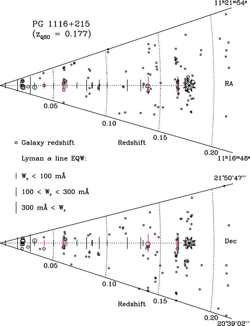
Figure 22: Comparison of the galaxy distribution within 50′ of PG 1116+215 to the redshifts of the Ly$\alpha$ and O VI absorbers measured in the STIS and FUSE spectra presented in this paper. Galaxies are indicated with open circles in a right ascension slice (top) and a declination slice (bottom). The size of the circle indicates proximity to the sight line; the largest circles show galaxies with projected distance $\rho\leq 500$ kpc, intermediate-size circles represent galaxies at 500 $<\rho\leq 1$ Mpc, and the smallest circles indicate galaxies at $\rho>1$ Mpc. Redshifts of Ly$\alpha$ lines are plotted with vertical lines on the sight line, and the length of the vertical line reflects the H I Ly$\alpha$ equivalent width as indicated in the key. The redshifts of the Ly$\alpha$ absorbers with corresponding O VI are highlighted in red.

Figures 21 and 22 compare the redshift distributions of the Ly$\alpha$ and O VI absorbers (including the weaker O VI lines identified at $z=0.04125$, 0.05895, 0.05928, and 0.06244) to the distribution of the galaxies along the line-of-sight to PG1116+215. Figure 21 presents histograms of the number of galaxies within 50′ and 30′ of the sight line as a function of redshift. Figure 22 shows the locations of the galaxies in right ascension and declination slices versus galaxy redshift (circles), as well as the redshifts of the Ly$\alpha$ and O VI absorption lines. The vertical lines of varying size plotted on the sight line in each slice of Figure 22 show the Ly$\alpha$ redshifts; the line size indicates the Ly$\alpha$ equivalent width following the legend in the figure. The redshifts of the Ly$\alpha$ absorbers containing O VI are highlighted in red. The largest circles in Figure 22 represent galaxies within 500 kpc in projection from the sight line, intermediate-size circles indicate galaxies with projected distances ($\rho$) ranging from 500 kpc to 1 Mpc, and small circles show galaxies at $\rho>$ 1 Mpc. For the O VI absorbers, Table 11 lists the galaxy with the smallest projected distance to the sight line and smallest velocity difference from the absorber.

Tripp et al. (1998) have shown that Ly$\alpha$ absorption-line systems are significantly correlated with galaxies in the direction of PG1116+215. Visual inspection of Figures 21 - 22 and Table 11 suggests that the O VI absorbers are strongly correlated with galaxies as well. For each of the seven O VI absorption lines identified in the PG1116+215 spectrum, we find at least one galaxy within $\rho\leq$ 750 kpc and $\Delta v\leq 600$ km s^-1; six out of the seven O VI systems have $\Delta v\leq$ 320 km s^-1. In addition, most of the O VI absorbers are found close to the peaks in the galaxy distribution. It is interesting that no O VI is positively identified near the prominent group of galaxies at $z\approx$ 0.0212; however, O VI at this redshift falls in a region of the FUSE spectrum that is heavily blocked by unrelated lines (see Figure 2), so it remains possible that O VI is simply hidden by blending in this case.

We have considered the possibility that our visual impression is just coincidental and that the O VI absorbers are actually randomly distributed with respect to the galaxies in the direction of PG 11116+215. To quantitatively assess this probability, we performed the following simple Monte Carlo statistical test. We carried out a large number of simulations in which we randomly distributed a number of absorbers along the sight line equal to the observed number of O VI systems, and then we determined the number of instances in which the simulations by chance showed the same number of absorbers as observed with $\rho\leq$ 750 kpc and $\Delta v\leq$ 350  km s^-1. Since associated absorption systems with $z\approx z_{\rm QSO}$ sometimes show strong evidence that the gas is close to the central engine of the QSO (e.g., Hamann & Ferland 1999; Yuan et al. 2002; Ganguly et al. 2003) and therefore is unrelated to the intervening absorbers, we excluded the two O VI absorbers observed toward PG1116+215 within 5000  km s^-1 of the QSO redshift from our first Monte Carlo analysis, and we set the maximum redshift for the random simulations to 5000  km s^-1 less than $z_{\rm QSO}$. We also treated the O VI lines at $z=$ 0.05895 and 0.05928 as a single “absorber” since these lines are separated by only $\sim$90  km s^-1 and therefore could easily arise in a single absorbering entity (e.g., a single galaxy). Finally, we required all of the random absorbers in the simulations to have $z\geq 0.02430$ because below that redshift, the FUSE spectrum is strongly blanketed with unrelated lines (which could easily hide weak O VI systems) and the physical radius covered by the galaxy redshift surveys is limited. With these exclusions, we have four intervening O VI absorbers in the PG 1116+215 spectrum (at $z$ = 0.04125, 0.059, 0.06244, and 0.13847). After running a total of $4\times 10^{5}$ Monte Carlo trials, we found 81 trials in which the randomly distributed systems showed the same number of absorbers within $\rho=$ 750 kpc and $\Delta v$ = 350 km s^-1 as the actually observed number. This indicates that the probability that the observed intervening O VI absorbers toward PG 1116+215 are randomly distributed with respect to the galaxies is 81/($4\times 10^{5})=2.0\times 10^{-4}$. We conclude that it is highly unlikely that the intervening O VI absorbers are randomly distributed with respect to galaxies in the direction of PG1116+215.

However, it is striking how well the two “associated” O VI lines toward PG 1116+215 line up with two of the most pronounced peaks in the galaxy distribution, so one might reasonably argue that the O VI absorbers at $z=0.16548$ and $z=0.17340$, despite their proximity to the QSO redshift, are also intervening. Consequently we have also carried out a Monte Carlo calculation in which the O VI lines within 5000 km s^-1 of $z_{\rm QSO}$ were included in the count, and the random distributions were allowed to extend all of the way to the QSO redshift. In this second set of Monte Carlo trials we found that the probability that the O VI lines are randomly distributed was even slightly smaller, $1.3\times 10^{-4}$. Therefore, our conclusion holds with this set of assumptions as well, and as we shall see in the next section our conclusions about baryonic content of the absorbers do not depend strongly on whether the velocity interval near the QSO is included in our calculations of the redshift path or $\Omega_{b}$(O VI).

Finally, we note that most of the Ly$\alpha$ absorbers along the sight line also occur at redshifts where there are peaks in the galaxy redshift distribution. Notable exceptions include the somce of the closer Ly$\alpha$ absorbers at $z=0.00493$, $0.01635$, and $0.04996$. At these lower redshifts, the galaxy redshift surveys cover a smaller volume of space than at higher redshifts, so the absence of galaxies at these redshifts will need to be tested more thoroughly. The generally good correlation of both Ly$\alpha$ and O VI with galaxy redshifts is a strong indication that the absorbers are truly intervening material rather than material ejected from QSOs at high velocities (e.g., Richards et al. 1999).

11 Baryonic Content of the Warm-Hot Intergalactic Medium

The detection of broad Ly$\alpha$ lines and O VI in the IGM demonstrates that there may be multiple baryon reservoirs in the low-redshift universe. Previous investigations have found that (d$N$/d$z$)${}_{\rm O\,VI}\approx 14\pm^{9}_{6}$ for absorbers with $W_{r}>50$ mÅ over an unblocked redshift path of 0.43 (Savage et al.  2002, and references therein). Toward PG 1116+215, we expect two and detect two O VI absorbers with $W_{r}>50$ mÅ over an unblocked redshift interval of $\Delta X_{\rm O\,{\sc VI}}=0.117$, which corresponds to (d$N$/d$z$)${}_{\rm O\,VI}\approx 17$. Adding in the weaker O VI absorbers along the sight line increases (d$N$/d$z$)${}_{\rm O\,VI}$ to $\sim 60$ for an equivalent width threshold $W_{r}\geq 30$ mÅ. The relatively high $S/N$ observations of H 1821+643 (Tripp et al. 2000) similarly indicate that d$N$/d$z$ increases significantly with increasing sensitivity to weak lines.

The baryonic content of the O VI systems is given by

$$\Omega_{b}({\rm O\,VI})=\frac{\mu_{H}~{}m_{\rm H}~{}H_{0}}{\rho_{c}~{}c}~{}\sum~{}\frac{{\rm N}_{i}{\rm(O\,VI)}}{f_{{}_{i}{\rm O\,VI}}~{}\Delta X_{i}~{}({\rm O/H})_{i}}~{}.$$ (7)

In this equation, $\Omega_{b}({\rm O\,VI})$ is inversely proportional to the ionization fraction of O VI and the metallicity of the gas. Savage et al. (2002) derived a value of $\Omega_{b}$(O VI) $>0.002h^{-1}_{75}$ assuming $f_{\rm O\,VI}<0.2$ and a metallicity of 0.1 solar for systems with $W_{r}>50$ mÅ. This estimate is comparable to the baryonic mass contained in stars and gas inside galaxies, $\Omega_{b}({\rm*,gas})\approx 0.0032\,h^{-1}_{75}$ (Fukugita 2003; Fukugita et al. 1998), and may rival the amount contained in the broad Ly$\alpha$ absorbers (see §9.2). While we cannot rule out a metallicity of 0.1 solar for the two stronger O VI absorbers toward PG 1116+215, the observational constraints are more readily satisfied for metallicities greater than $\sim 0.5$ solar. As a result, the baryonic estimate might decrease slightly if the O VI systems along other sight lines have similar metallicities. We note that Savage et al. (2002) favor a metallicity of $\sim 0.4$ solar for the $z=0.06807$ O VI absorber toward PG 0953+415. The ionization fraction of O VI rarely exceeds 0.2 (see Tripp & Savage 2000; Sembach et al. 2003), so the above estimate for $\Omega_{b}$(O VI) also has a strong dependence on the value of $f_{\rm O\,VI}$.

A summary of the baryonic content of the broad Ly$\alpha$ and O VI absorbers can be found in Table 12. For both types of absorbers, we list values of $\Omega_{b}$ and $\Omega_{b}^{\prime}$. The baryonic content does not depend strongly on whether or not the 5000  km s^-1 interval nearest PG 1116+215 is included in the calculations. For the Ly$\alpha$ absorbers, we list the values of $\Omega_{b}$(BLy$\alpha$) for all of the broad lines observed (${\rm b}\gtrsim 40$  km s^-1) as well as the values for the more restricted line width interval of $40\lesssim{\rm b}\lesssim 100$  km s^-1 considered in §9.2. O VI values for two limiting equivalent widths ($W_{r}\geq 30$ and 50 mÅ) are given. We also tabulate an average value of $\Omega_{b}$(O VI) $\gtrsim 0.0027h_{75}^{-1}$ for 13 absorbers with $W_{r}\geq 50$ mÅ along 6 lines of sight assuming a metallicity of 0.1 solar and an O VI ionization fraction $f_{\rm O\,VI}<0.2$. References for the other lines of sight used in this summary can be found in the notes for the table.

Different types of O VI systems may have different physical properties. The two primary O VI absorbers toward PG 1116+215 at $z=0.13847$ and $z=0.16548$ clearly have very different ionization structures. Photoionization may play a role in the production of O VI in these systems, though it cannot be the primary ionization mechanism if the O VI and lower ionization stages observed are co-spatial as implied by the similarities in their kinematics. The O VI absorption associated with the broad Ly$\alpha$ absorbers at $z=0.04125$ and $0.06244$ may trace yet another type of environment. For these systems, the Ly$\alpha$ and O VI line shapes are consistent with thermal broadening in hot gas. It is particularly interesting that the O VI line widths in the $z=0.06244$ system and in the $z=0.31978$ absorber toward PG 1259+593 are narrow and in roughly the right proportion to the H I line widths to be due to thermal broadening in hot, collisionally ionized gas. If instead the lines had been produced by photoinization, the cloud sizes required to reproduce the O VI columns would have been large ($\gtrsim 0.5$ Mpc), and the lines would have been broadened considerably by the Hubble flow. The detection of H I in high temperature gas has profound implications for the baryonic content of the gas since the amount of related ionized gas implied is very large indeed (see §9.2).

Obtaining high quality data of the type used in this study for other sight lines is essential for revealing weak features like the O VI absorption in these broad Ly$\alpha$ systems. Quantifying the baryonic content of the O VI and broad Ly$\alpha$ absorbers more precisely will require estimates of the O VI ionization fractions ($f_{i}$) and gas metallicities (O/H) in the different types of systems rather than assuming common values for all cases. There are two measurements that are particularly valuable for determinations of the O VI absorber properties and constraining the value of $(f_{\rm O\,VI})~{}({\rm O/H})$. The first is an accurate assessment of the strength and kinematics of C IV absorption in these systems. The ratio N(O VI)/N(C IV) is a powerful diagnostic of the primary ionization mechanism for the highly ionized gas. When the kinematical information in the profiles indicate that a direct comparison of column densities of the two species is meaningful, the ratio can be used to discriminate between collisional ionization and photoionization. For PG 1116+215, the existing HST/STIS E230M spectrum does not cover the C IV absorption associated with the two strong O VI absorbers at $z=0.13847$ and $z=0.16548$. The STIS/E140M covers some of the lower redshift absorbers but the data are not of sufficient $S/N$ to detect the C IV lines in most cases. In the one case where C IV is possibly detected (e.g., $z=0.05928$), the comparable strengths of the O VI and C IV lines supports photoionization as the preferred ionization mechanism (see §8.2). The second type of measurement is an observation of the extreme-ultraviolet lines of O III $\lambda 832.927$ and O IV $\lambda 787.711$, and O V $\lambda 629.730$ for those O VI absorbers at redshifts sufficiently high to place the lines in the wavelength range covered by FUSE ($\lambda>912$ Å, $z\gtrsim 0.2-0.4$). Having access to several stages of ionization may allow determinations of both the ionization and metallicity of the gas. Additional extreme-ultraviolet diagnostics such as Ne VIII $\lambda\lambda 770.409,780.324$ and Mg X $\lambda\lambda 609.790,624.950$ are also valuable in assessing whether the gas is collisionally ionized at high temperatures (see Savage et al. 2004). Unfortunately, none of the O VI absorbers toward PG 1116+215 occur at redshifts high enough to observe the EUV lines with the FUSE LiF channels or with STIS.

Many of the low-redshift O VI absorption systems are clearly multi-phase in nature. This conclusion holds for the $z=0.13847$ absorber toward PG 1116+215 as well as absorbers toward H 1821+643, (Tripp et al. 2000), PG 1259+593 (Richter et al. 2004), and possibly PG 0953+415 (Savage et al. 2002). Multiple ionization mechanisms are required to explain the observed amounts of O VI and lower ionization stages in the gas. The PG 1116+215 $z=0.13847$ absorber is particularly interesting in this regard since it has the highest H I content of the low-redshift O VI absorbers studied to date and yet has an O VI column density comparable to those of many of the other systems. As mentioned in §6.3, its ionization properties bears some resemblance to those of ionized high-velocity clouds near the Milky Way. Gnat & Sternberg (2004) have modeled the ionization pattern expected for photoionized dark matter dominated mini-halos in the Local Group (see also Kepner et al. 1999) and have suggested that some of the ionized high velocity gas near the Milky Way could occur in the outer envelopes of low surface brightness dwarf galaxies. Their model does not produce significant amounts of O VI, which must still be produced by other means. Locally, the O VI could occur in warm-hot gas interfaces caused by interactions of the high-velocity gas with a hot ($T\sim 10^{6}$ K) low-density ($n\lesssim 10^{-4}$ cm^-3) Galactic corona or Local Group medium (Sembach et al. 2003). Similar interactions of warm and hot gases are expected to occur as the IGM evolves, especially in regions where galaxies have formed.

We conclude by noting that our results demonstrate that broad Ly$\alpha$ and O VI absorbers could be substantial reservoirs of baryons in the low-redshift universe. In some cases, these may be one and the same. Narrow Ly$\alpha$ absorbers also contribute significantly to the total baryon budget. For example, Penton et al. (2004) have estimated that the baryonic content of the Ly$\alpha$ clouds in the low-redshift universe is $\approx 40\pm 10$% of the total baryonic mass, under the assumption that the Ly$\alpha$ clouds are photoionized. Understanding the ionization of the Ly$\alpha$ and O VI clouds will lead to a more rigorous accounting of the baryon content of the clouds. Comsological hydrodynamic simulations predict that stronger Ly$\alpha$ absorbers should be more strongly correlated with galaxies than weaker absorbers, and that there should be both photoionized and collisionally ionized systems (Davé et al. 1999). Quantifying these statements both observationally and theoretically will be a major challenge for astronomers in the coming years.

12 Summary

The results of our HST/STIS and FUSE study of the Ly$\alpha$ and O VI absorption systems along the PG 1116+215 sight line are as follows.

1) We detect 25 Ly$\alpha$ absorbers along the sight line at rest-frame equivalent widths $W_{r}\gtrsim 30$ mÅ, yielding (d$N$/d$z$)${}_{{\rm Ly}\alpha}=154\pm 18$ over an unblocked redshift path $\Delta X_{{\rm Ly}\alpha}=0.162$. We also detect two weak Ly$\alpha$ features with $W_{r}=15-20$ mÅ. Most, if not all, of these are intergalactic systems. The metal-line absorption systems at $z\approx 0.166$ and $z=0.17340-0.17360$ could be associated with the quasar, but we believe that it is just as likely that they are truly intervening systems since they occur at redshifts corresponding to peaks in the galaxy redshift distribution along the sight line.

2) Some of the Ly$\alpha$ absorbers have broad line widths (b $\gtrsim 40$  km s^-1). The detection of narrow O VI absorption in at least one broad Ly$\alpha$ absorber along the sight line ($z=0.06244$) supports the idea that thermal broadening in hot gas could account for much of the breadth of the H I lines. If the H I line widths are dominated by thermal broadening at $T>10^{5}$ K, the amount of baryonic material in these absorbers is enormous because the ionization corrections required to account for the observed H I columns are large.

3) We find d$N$/d$z$ $\approx 50$ for broad Ly$\alpha$ absorbers with $W_{r}\gtrsim 30$ mÅ and ${\rm b}\geq 40$  km s^-1. This number drops to d$N$/d$z$ $\approx 37$ if the line widths are restricted to $40\leq{\rm b}\leq 100$  km s^-1. As much as half the baryonic mass in the low-redshift universe could be contained in broad collisionally-ionized Ly$\alpha$ systems.

4) We detect O VI absorption in several of the Ly$\alpha$ clouds along the sight line. Two detections at $z=0.13847$ and $z=0.16548$ are confirmed by the presence of other ions at these redshifts, while the detections at $z=0.04125$, $0.05895$, $0.05928$, and $0.06244$ are based upon the Ly$\alpha$ and O VI detections alone. We find (d$N$/d$z$)${}_{\rm O\,VI}\approx 17$ for O VI absorbers line with $W_{r}>50$ mÅ toward PG 1116+215.

5) Compiling the information available for 13 low-redshift O VI absorbers with $W_{r}\geq 50$ mÅ along 5 sight lines yields (d$N$/d$z$)${}_{\rm O\,VI}\approx 14$ and $\Omega_{b}$(O VI) $\gtrsim 0.0027h_{75}^{-1}$, assuming a metallicity of 0.1 solar and an O VI ionization fraction $f_{\rm O\,VI}\leq 0.2$. The implied baryonic content of the O VI absorbers is comparable to the baryonic mass contained in stars and gas inside galaxies.

6) We detect metal-line absorption in the $z=0.13847$ system. Species detected include H I, C II-III, N II-III, N V, O I, O VI, and Si II-IV. The numerous Lyman-series lines and weak Lyman limit allow us to estimate N(H I) = $(1.57\pm^{0.18}_{0.14})\times 10^{16}$ cm^-2 in this system. Investigation of the ionization of this system indicates that the absorber is multi-phase in nature. The presence of O VI likely requires collisional ionization, while the ionization pattern seen in the lower ionization stages can be explained in part by photoionization in a low-density plasma. Regardless of the ionization mechanism, the absorber is composed mainly of ionized gas.

7) We detect a group of Ly$\alpha$ lines near $z=0.166$. Three absorbers within a velocity interval of 500  km s^-1 contribute to the majority of the overall Ly$\alpha$ absorption. Additional weak Ly$\alpha$ components are also present in this velocity interval.

8) The $z=0.16548$ Ly$\alpha$ absorber contains O VI and possibly N V. The O VI absorption appears to consist of at least three components, two of which are narrow (b $<10$  km s^-1). If the gas is photoionized, a high ionization parameter is required ($\log U\approx-0.5$, $n_{\rm H}\sim 10^{-6}$ cm^-3) and the cloud must be large ($L\sim 1$ Mpc). If collisional processes also contribute to the ionization of the cloud, these constraints can be relaxed. This absorber resembles the $z=0.14232$ absorber toward PG 0953+415. Observations of C IV would help to solidify statements about the ionization properties of this absorber.

9) The $z=0.16610$ Ly$\alpha$ absorber contains C II, C III, and Si II. Its ionization properties are marginally consistent with photoionization in a moderate ionization plasma ($\log U\approx-2.63$, $n_{\rm H}\sim 1.6\times 10^{-4}$ cm^-3). Increasing the relative abundance of silicon to carbon compared to the solar ratio would improve the agreement of the observed and predicted column densities of C II and Si II.

10) We find a strong correlation of the redshifts of the Ly$\alpha$ and O VI absorbers with the redshifts of galaxies along the sight line. Monte-Carlo simulations indicate that the probability of a random distribution of O VI absorbers is $<2\times 10^{-4}$. None of the intervening O VI absorbers is nearer than $\sim 100\,h_{75}^{-1}$ kpc to a known galaxy, and most are farther than $\sim 600\,h_{75}^{-1}$. This suggests that the O VI arises in intragroup gas rather than in the extended halos of large galaxies.

11) A few Ly$\alpha$ clouds along the sight line lie at redshifts where no galaxies have yet been detected ($z=0.00493$, $0.01635$, $0.04996$). Deeper galaxy searches at these and other redshifts would help to further elucidate the relationship (or lack thereof) of the absorbers to galaxies.

Figure 1: FUSE and STIS ultraviolet spectra of PG 1116+215 obtained for this study. The data have been binned into 0.2 Å samples for this illustration. The FUSE data segments plotted in the top panel are indicated above the spectrum. The flux levels implied by the FUSE data are about 30% higher than those in the STIS spectrum (see text); the flux discrepancy does not affect the line analyses in this study. The flux level sag in the FUSE LiF2A data between 1110 and 1150 Å is caused in part by an uncalibrated shadow cast by grid wires above the FUSE detector. Asterisks mark the locations of small gaps in wavelength coverage between the STIS echelle orders at longer wavelengths.

Figure 2: See caption at end of figure.

Figure 2 (continued): See caption at end of figure.

Figure 2 (continued): See caption at end of figure.

Figure 2 (continued): See caption at end of figure.

Figure 2 (continued): Fully reduced FUSE spectra of PG 1116+215 as a function of heliocentric wavelength between 915 and 1187 Å. Data from two channels are shown at most wavelengths, with SiC data shown at $\lambda\lesssim 1000$ Å, and LiF data shown at $\lambda\gtrsim 1000$ Å. SiC data are also shown in the LiF coverage gap near 1070–1090 Å. The detector segments shown are identified in the lower corners of each panel. The data have a spectral resolution of $\approx 20-25$  km s^-1 (FWHM). Line detections are denoted by tick marks above the spectra. Line identifications for these detections are listed at the right hand side of each panel. Redshifts (in parentheses) are indicated for intergalactic lines. Rest wavelengths are indicated for interstellar lines. Interstellar molecular hydrogen lines are labeled according to their rotational and vibrational levels as described in the text. In cases where the +184  km s^-1 high-velocity interstellar feature is present, an offset tick mark is attached to the primary tick mark at the rest wavelength of the line. Several fixed-pattern noise (FPN) and unidentified (UID) features are also labeled. The dashed horizontal line in panel g illustrates the continuum placement longward of the Lyman-limit system at $z=0.13847$.

Figure 3: See caption at end of figure.

Figure 3 (continued): See caption at end of figure.

Figure 3 (continued): See caption at end of figure.

Figure 3 (continued): See caption on next page.

Figure 3 (continued): Fully reduced HST/STIS E140M spectra of PG 1116+215 as a function of heliocentric wavelength between 1167 and 1709 Å. The data have a 2-pixel (FWHM) spectral resolution of $\approx 6.5$  km s^-1. We have binned the data into two pixel bins for clarity, but all measurements were conducted on the fully sampled data. Labels are similar to those in Figure 2.

Figure 4: See caption on next page.

Fig. 4. — Portions of the fully reduced HST/STIS E230M spectra of PG 1116+215 as a function of heliocentric wavelength between 2250 and 2851 Å. The data have a 2-pixel (FWHM) spectral resolution of $\approx 10$  km s^-1. The unbinned data are plotted at the nominal sampling interval of $\approx 5$  km s^-1. Labels are similar to those in Figure 2.

Figure 5: A comparison of the HST/STIS E140M and GHRS G140L spectra of PG 1116+215 between 1220 and 1500 Å. Top: GHRS G140L spectra obtained with FP-SPLIT procedures by Tripp et al. (1998). The spectra have a total exposure time of 3.5 hours and a spectral resolution of $\approx 160$  km s^-1 (FWHM). Middle: STIS E140M spectra of PG 1116+215 convolved with a Gaussian smoothing kernel having FWHM = 160  km s^-1 and resampled to the GHRS wavelength vector. The resulting spectrum looks very similar to the GHRS G140L spectrum. Bottom: Full-resolution STIS E140M spectra of PG 1116+215 binned by 2 pixels. Expanded regions of this plot can be found in Figure 3.

Figure 6: A portion of the FUSE SiC2 spectrum of PG 1116+215 in the wavelength region covering the redshifted lines of O II $\lambda\lambda 832.757,833.329,834.466$ and O III $\lambda 832.927$ in the $z=0.13847$ metal-line system. The heliocentric wavelengths of the redshifted oxygen lines are indicated with tick marks at the top of the figure. Galactic lines of H I $\lambda 949.743$, O I $\lambda 948.468$, and several H₂ lines in the Lyman series 14-0 and Werner series 3-0 vibrational bands are labeled immediately above the spectrum. For the Galactic O I line, the three ticks indicate components at negative intermediate velocity ($-44$  km s^-1), zero velocity, and high positive velocity (+184  km s^-1). The H₂ lines indicated include $\lambda\lambda 946.978$ (14-0) R(1), 947.111 (3-0) R(2), 947.421 (3-0) Q(1), 947.513 (14-0) P(1), 948.419 (3-0) R(3), and 948.468 (14-0) R(2), all of which occur in the $-44$  km s^-1 interstellar component along the sight line. The expected absorption due to the two interstellar H₂ lines near 948.3 Å is shown as a heavy smooth curve overplotted on the spectrum. Terrestrial airglow emission between 949.5 and 949.9 Å is indicated with a crossed circle below the spectrum.

Figure 7: See caption on next page.

Fig. 7. — Ly$\alpha$ absorbers toward PG 1116+215. The redshifts of Ly$\alpha$ features are indicated for the main absorption and for the “satellite” absorbers at $z=0.05928$, 0.16548, 0.16580, 0.16686, and 0.17340. Other ISM and IGM features are identified by species. A portion of the spectrum containing Galactic Si II $\lambda 1304.370$ absorption near the $z=0.07188$ absorber has been omitted for clarity. Gaussian components fit to each intervening Ly$\alpha$ line are overplotted as smooth curves. See text for details.

Figure 8: Normalized absorption profiles for the $z=0.04125$ absorption-line system. The vertical dashed line indicates the systemic velocity of the Ly$\alpha$ line.

Figure 9: Normalized absorption profiles for the $z=0.05895,0.05928$ absorption-line system. The velocity scale is centered on the systemic velocity of the Ly$\alpha$ absorber at $z=0.05895$. The second vertical line indicates the velocity of the system at $z=0.05928$.

Figure 10: Normalized absorption profiles for the $z=0.06244$ absorption-line system. The vertical dashed line indicates the systemic velocity of the Ly$\alpha$ line.

Figure 11: Continuum-normalized absorption profiles for lines in the absorption-line system at $z=0.17340-0.17360$.

Figure 12: Continuum-normalized H I lines in the $z=0.13847$ absorber. The Ly$\alpha$ profile is from HST/STIS. All others are from the FUSE LiF1 channel.

Figure 13: Single-component curve of growth for the H I Lyman-series lines in the $z=0.13847$ metal-line system. The STIS Ly$\alpha$ measurement is shown as a filled square data point. The FUSE measurements for the other lines are represented by either filled circles (LiF1, SiC1) or open circles (LiF2, SiC2). Error bars are $1\sigma$ estimates. The Ly$\theta$ line was not used in the fit because it is partially blended with a Galactic H₂ line (see Table 5). The best fit COG has N(H I) = $(1.57\pm^{0.18}_{0.14})\times 10^{16}$ cm^-2 (log N = $16.20\pm^{0.05}_{0.04}$) and b = $22.4\pm 0.3$  km s^-1.

Figure 14: See caption on next page

Fig. 14. — Continuum-normalized metal lines in the $z=0.13847$ absorber. Both FUSE and STIS data are shown. The FUSE data are from the SiC2 or LiF1 channels. The three detections of O VI $\lambda 1031.926$ are shown at the bottom of the right hand panel. The STIS data for the O VI line has been binned into 2-pixel samples since the spectrum is noisy at these wavelengths (see Figure 3).

Figure 15: Predicted column densities for the photoionization model of the $z=0.13847$ system. Relevant quantities for the physical conditions in this plane-parallel, uniform density slab of gas (pressure, temperature, density, ionization parameter, total hydrogen column density, and cloud thickness) are plotted along the x axes. See text for details.

Figure 16: Absorption lines in the $z\approx 0.166$ absorbers. Three Ly$\alpha$ absorbers are located within 400  km s^-1 of each other at $z=0.16548$, 0.16610, and 0.16686. These redshifts are indicated by the vertical dotted lines.

Figure 17: Single-component curve of growth for the H I Lyman-series lines in the $z=0.16610$ absorber. The STIS Ly$\alpha$ and Ly$\beta$ measurements are shown as filled square data points. The FUSE LiF2 measurement for the Ly$\epsilon$ line is represented by the open circle. Error bars are $1\sigma$ estimates. A small residual amount of Ly$\alpha$ absorption ($\sim$60 mÅ) was not included in the fit since it is outside the velocity range of the Ly$\beta$ absorption (see text and Figure 7). The best fit COG has N(H I) = $(4.17\pm^{0.59}_{0.48})\times 10^{14}$ cm^-2 (log N = $14.62\pm^{0.06}_{0.05}$) and b = $22.0\pm 0.9$  km s^-1.

Figure 18: Apparent column density profiles for the two O VI lines and the H I Ly$\alpha$ line in the $z=0.16548$ absorber constructed from the STIS absorption-line data shown in Figure 16. Error bars are $1\sigma$ estimates. Top: Data points for the $\lambda 1031.926$ line are filled circles. Data points for the $\lambda 1037.617$ line are open circles. To reduce confusion, the $\lambda 1031.926$ data points have been connected with straight lines. Bottom: The Ly$\alpha$ line.

Figure 19: Predicted column densities for the photoionization model of the $z=0.16610$ system. Relevant quantities for the physical conditions in this plane-parallel, uniform density slab of gas (pressure, temperature, density, ionization parameter, total hydrogen column density, and cloud thickness) are plotted along the x axes. Observed values for N(C III) and N(Si III) are shown with the filled points. The errors on the observed column densities are comparable to the size of the symbols. See text for details.

Figure 20: Line width versus H I column density for the Ly$\alpha$ absorbers identified along the PG 1116+215 and PG 1259+593 sight lines. The corresponding temperature for a single, thermally-broadened line is shown on the right side of the plot. The PG 1116+215 data are shown as filled squares with $1\sigma$ error bars; in some cases the error bars are smaller than the symbol size. The PG 1259+593 data from Richter et al. (2004) are shown as circles; open circles indicate less reliable values. The solid curve indicates the relation between b-value and column density for a Gaussian line with a central optical depth of 10%. Weak, broad Ly$\alpha$ lines in the region to the left of this curve would be difficult to detect in the data used for this study.

Figure 21: Histogram of 103 galaxy redshifts within 50′ of PG 1116+215 at $z<0.1765$. The histogram bins have a width $\Delta z=0.001$. Galaxies within 30′ are highlighted with filled bins. The redshifts of the Ly$\alpha$ and O VI absorption systems observed along the sight line are indicated by vertical tick marks above the histogram. The Ly$\alpha$ absorbers are separated into narrow (${\rm b}\lesssim 40$  km s^-1) and broad (${\rm b}\gtrsim 40$  km s^-1) absorbers. The tick marks for the $z=0.05895,0.05928$ and $z=0.17340,0.17360$ pairs of lines blend together.

Table 1: FUSE Observations of PG 1116+215

Dataset	Date	# Exp.	LiF1 / SiC1		LiF2 / SiC2		Aperture
	(U.T. Start)		Ttot	Tngt	Ttot	Tngt
			(ksec)	(ksec)	(ksec)	(ksec)
P1013101	2000-Apr-28	07	11.0	11.0	11.0	11.0	$30\arcsec\times 30\arcsec$
P1013102	2001-Apr-22	05	11.1	09.4	11.1	09.4	$30\arcsec\times 30\arcsec$
P1013103	2001-Apr-22	06	08.4	06.3	08.4	06.3	$30\arcsec\times 30\arcsec$
P1013104	2001-Apr-23	05	11.2	09.5	11.2	09.5	$30\arcsec\times 30\arcsec$
P1013105	2001-Apr-23	20	35.0	27.8	35.1	27.8	$30\arcsec\times 30\arcsec$

Table 2: HST/STIS E140M and E230M Observations of PG 1116+215

Program	Grating/Tilt	Dataset	Date	# Exp.	Ttot	Slit
			(U.T. Start)		(ksec)
GO-8097	E140M/1425	O5A301010–O5A301020	2000-May-20	9	12.6	$0.2\arcsec\times 0.06\arcsec$
GO-8097	E140M/1425	O5A302010–O5A302020	2000-May-15	5	07.3	$0.2\arcsec\times 0.06\arcsec$
GO-8165	E140M/1425	O5E701010–O5E701070	2000-Jun-22	7	10.0	$0.2\arcsec\times 0.06\arcsec$
GO-8165	E140M/1425	O5E702010–O5E702070	2000-Jun-30	7	10.0	$0.2\arcsec\times 0.06\arcsec$
GO-8097	E230M/2415	O5A302030–O5A302050	2000-May-15	4	05.6	$0.2\arcsec\times 0.06\arcsec$

Table 3: Interstellar Line Cross Reference for Lines

Species	$\lambda$(Å)	$\log f\lambda$	ID	Comments
H I	0917.181	$-0.178$	2a-1	Additional H I blanketing at $\lambda<917$ Å
H I	0918.129	$-0.072$	2a-2	HVC component at +184  km s-1
H I	0919.351	0.043	2a-3	HVC component at +184  km s-1
H I	0920.963	0.170	2a-4	HVC component at +184  km s-1
O I	0921.857	$-0.001$	2a-5
H I	0923.150	0.135	2a-6	HVC component at +184  km s-1
H2 L17R7	0924.641	0.574	2a-7
O I	0924.950	0.155	2a-8
O I	0925.446	$-0.484$	2a-9
H I	0926.226	0.294	2a-10	HVC component at +184  km s-1
O I	0929.517	0.329	2a-11
H I	0930.748	0.475	2a-12	HVC component at +184  km s-1
H2 L16R1	0931.730	0.850	2a-13
H2 L16R3	0935.573	0.789	2a-14
O I	0936.630	0.534	2a-15
H I	0937.803	0.688	2a-16	HVC component at +184  km s-1
H2 L15R1	0939.122	0.793	2a-17
H2 L15P1	0939.706	0.437	2b-1
H2 W3R1	0946.384	1.082	2b-2	Blend with H2 W3R0
H2 W3R0	0946.423	1.757	2b-2	Blend with H2 W3R1
H2 L14R1	0946.978	1.271	2b-3	Blend with H2 W3R2
H2 W3R2	0947.111	1.103	2b-3	Blend with H2 L14R1
H2 W3Q1	0947.421	1.406	2b-4	Blend with H2 L14P1
H2 L14P1	0947.513	0.521	2b-4	Blend with H2 W3Q1
H2 W3R3	0948.419	1.085	2b-5
O I	0948.685	0.778	2b-6	HVC component at +184  km s-1?
H I	0949.743	0.946	2b-7	HVC component at +184  km s-1
O I	0950.885	0.176	2b-8	HVC component at +184  km s-1
N I	0952.303	0.338	2b-9	Blend with N I $\lambda\lambda 952.415,952.532$
N I	0953.415	1.091	2b-10
N I	0953.655	1.372	2b-11
N I	0953.970	1.499	2b-12
N I	0954.104	0.582	2b-13
H2 L13R1	0955.064	0.974	2b-14
H2 L13P1	0955.708	0.608	2b-15
H2 L13R2	0956.578	0.945	2b-16
H2 L13P2	0957.650	0.661	2b-17
H2 L12R0	0962.976	1.109	2c-1
H2 L12R1	0963.607	0.841	2c-2
P II	0963.801	3.148	2c-3	HVC component at +184  km s-1
H2 W2R0	0964.981	0.870	2c-4	Blend with H2 L12R2 and W2R1
H2 L12R2	0965.045	0.189	2c-4	Blend with H2 W2R0 and W2R1
H2 W2R1	0965.062	1.528	2c-4	Blend with H2 W2R0 and L12R2
H2 W2R2	0965.791	1.481	2c-5
H2 W2Q1	0966.094	1.529	2c-6
H2 W2R3	0966.779	0.864	2c-7
H2 W2Q2	0967.278	1.530	2c-8
H2 L12R3	0966.673	1.356	2c-9
H2 W2P2	0968.292	0.847	2c-10
H2 W2Q3	0969.047	1.533	2c-11
O I	0971.738	1.052	2c-12
H I	0972.537	1.450	2c-13
H2 L11R2	0974.156	1.108	2c-14
O I	0976.448	0.509	2c-15
C III	0977.020	2.869	2c-16
H2 L11P3	0978.217	0.821	2c-17
H2 L10R0	0981.437	1.310	2d-1
H2 L10R1	0982.073	1.130	2d-2
H2 L10P1	0982.835	0.822	2d-3
H2 L10R2	0983.589	1.056	2d-4
H2 L10P2	0984.862	0.907	2d-5
H2 W1R0	0985.632	1.838	2d-6	Blend with H2 W1R1
H2 W1R1	0985.642	1.525	2d-6	Blend with H2 W1R0
H2 W1R2	0986.241	1.418	2d-7
H2 W1Q1	0986.796	1.557	2d-8
H2 W1R3	0987.445	1.415	2d-9
H2 L10P3	0987.767	0.943	2d-10
H2 W1Q2	0987.972	1.558	2d-11
O I	0988.773	1.662	2d-12
N III	0989.799	2.085	2d-13
Si II	0989.873	2.228	2d-14
H2 L9R0	0991.376	1.413	2d-15	Blend with H2 W1P3
H2 W1P3	0991.378	1.060	2d-15	Blend with H2 L9R0
H2 L9R1	0992.014	1.257	2d-16
H2 L9P1	0992.808	0.893	2d-17
H2 L9R2	0993.547	1.227	2d-18
H2 L9P2	0994.871	0.934	2d-19
H2 L9R3	0995.970	1.219	2d-20
H2 L8R0	1001.821	1.426	2e-1
H2 L8R1	1002.449	1.264	2e-2
H2 L8P1	1003.294	0.933	2e-3
H2 L8R2	1003.982	1.225	2e-4
H2 L8P2	1005.390	1.002	2e-5
H2 L8R3	1006.411	1.202	2e-6
H2 W0R1	1008.498	1.317	2e-7	Blend with H2 W0R0
H2 W0R0	1008.552	1.646	2e-7	Blend with H2 W0R1
H2 W0R2	1009.024	1.197	2e-8
H2 W0Q1	1009.771	1.393	2e-9
H2 W0R3	1010.129	1.143	2e-10	$W_{\lambda}=30$ mÅ; used for comparison with H2 W3R3 in Figure 6
H2 W0Q2	1010.938	1.394	2e-11
H2 W0P2	1012.169	0.748	2e-12
S III	1012.495	1.647	2e-13
H2 L7R0	1012.810	1.476	2e-14	Blend with H2 W0Q3
H2 W0Q3	1012.680	1.396	2e-14	Blend with H2 L7R0
H2 L7R1	1013.435	1.318	2e-15
H2 L7P1	1014.326	0.948	2e-16
H2 W0P3	1014.504	0.924	2e-16
H2 L7R2	1014.974	1.286	2e-17
H2 L7P2	1016.458	1.017	2e-18
H2 L7R3	1017.422	1.271	2e-19
Si II	1020.699	1.234	2f-1
H2 L6R0	1024.372	1.470	2f-2
H2 L6R1	1024.987	1.305	2f-3
H I Ly$\beta$	1025.722	1.909	2f-4	$\oplus$ airglow emission present
H2 L6P2	1028.104	1.032	2f-5
H2 L6P3	1031.191	1.061	2f-8	$W_{\lambda}=30$ mÅ; used for comparison with H2 W3R3 in Figure 6
O VI	1031.926	2.136	2f-9	HVC component at +184  km s-1
C II	1036.337	2.088	2f-10	HVC at +184  km s-1 blends with C II∗ $\lambda 1037.018$
H2 L5R0	1036.545	1.448	2f-11
C II∗	1037.018	2.088	2f-12	Blend with C II $\lambda 1036.337$ HVC at +184  km s-1
H2 L5R1	1037.149	1.271	2f-13
O VI	1037.617	1.834	2f-14	HVC component at +184  km s-1
H2 L5P1	1038.157	0.952	2f-15
H2 L5R2	1038.689	1.235	2f-16
O I	1039.230	0.974	2f-17
H2 L5P2	1040.366	1.006	2f-18
H2 L5P3	1043.502	1.049	2g-3	Blended with H I Ly$\nu$ at $z=0.13847$
Ar I	1048.220	2.440	2g-7
H2 L4R0	1049.367	1.388	2g-9
H2 L4R1	1049.960	1.210	2g-10
H2 L4P1	1051.033	0.910	2g-11	Blend with H I Ly$\theta$ at $z=0.13847$
H2 L4R2	1051.498	1.165	2g-12	$W_{\lambda}=40$ mÅ; used for comparison with H2 L14R2 in Figure 6
H2 L4P2	1053.284	0.976	2g-13
H2 L4R3	1053.976	1.146	2g-14
Fe II	1055.262	0.812	2g-17
H2 L4P3	1056.472	1.004	2g-18	Weak line
H2 L3R0	1062.882	1.276	2h-2
Fe II	1063.176	1.765	2h-3
H2 L3R1	1063.460	1.101	2h-4
Fe II	1063.972	0.704	2h-5
H2 L3P1	1064.606	0.780	2h-6
H2 L3R2	1064.996	1.057	2h-7	$W_{\lambda}=37$ mÅ; used for comparison with H2 L14R2 in Figure 6
Ar I	1066.660	1.857	2h-8
H2 L3P2	1066.905	0.877	2h-9
H2 L3R3	1067.479	1.033	2h-10
H2 L2R0	1077.140	1.092	2h-13
H2 L2R1	1077.700	0.927	2h-14
H2 L2P1	1078.927	0.624	2h-15
H2 L2R2	1079.226	0.868	2h-16
Fe II	1081.875	1.134	2i-2
N II	1083.994	2.079	2i-3	HVC component at +184  km s-1
H2 L1R0	1092.195	0.809	2i-4
H2 L1R1	1092.732	0.627	2i-5
H2 L1P1	1094.052	0.334	2i-9
H2 L1R2	1094.244	0.553	2i-10
Fe II	1096.877	1.554	2i-12	HVC component at +184  km s-1 ?
H2 L0R0	1108.127	0.264	2j-2
H2 L0R1	1108.633	0.076	2j-3
H2 L0P1	1110.063	–0.197	2j-4
H2 L0R2	1110.120	0.014	2j-5
Fe II	1112.048	0.695	2j-6
Fe II	1121.975	1.512	2k-1
Fe III	1122.524	1.786	2k-2
Fe II	1125.448	1.244	2k-3
Fe II	1127.098	0.102	2k-5	May blend with N III at $z=0.13847$
Fe II	1133.665	0.728	2k-6
N I	1134.165	1.219	2k-7
N I	1134.415	1.512	2k-8
N I	1134.980	1.674	2k-9
Fe II	1142.366	0.661	2l-2
Fe II	1143.226	1.342	2l-3	HVC component at +184  km s-1 ?
Fe II	1144.938	1.978	2l-4	HVC component at +184  km s-1
P II	1152.818	2.451	2l-7
Si II	1190.416	2.541	3b-1	HVC component at +184  km s-1
Si II	1193.290	2.842	3b-2	Blend with S III $\lambda 1193.208$, HVC at +184  km s-1
Mn II	1197.184	2.414	3b-4	Tentative identification
N I	1199.550	2.199	3b-5
N I	1200.223	2.018	3b-6
N I	1200.710	1.715	3b-7
Si III	1206.500	3.293	3b-10	HVC component at +184  km s-1
H I Ly$\alpha$	1215.670	2.704	3c-3	$\oplus$ airglow emission present
Mg II	1239.925	–0.106	3d-4	Weak line, Mg II $\lambda 1240.395$ absent
S II	1250.584	0.832	3e-2
S II	1253.805	1.136	3e-3	HVC at +184  km s-1 blends with Ly$\alpha$ at $z=0.03223$
S II	1259.518	1.320	3e-5	HVC at +184  km s-1 blends with Si II $\lambda 1260.422$
Si II	1260.422	3.171	3e-6
C I	1277.245	2.037	3f-2
O I	1302.168	1.796	3g-3
Si II	1304.370	2.052	3g-4
Ni II	1317.217	2.284	3h-3	HVC component at +184  km s-1?
C I	1328.833	2.003	3i-2	Weak line
C II	1334.532	2.234	3i-3	HVC component blends with C II${}^{*}\lambda 1335.708$
C II∗	1335.708	2.188	3i-4	No HVC component visible
Ni II	1370.132	2.023	3k-1
Si IV	1393.755	2.854	3l-1	HVC component at +184  km s-1
Si IV	1402.770	2.552	3l-2	HVC component at +184  km s-1
Ni II	1454.842	1.672	3o-1	Tentative identification
Si II	1526.707	2.307	3r-2	HVC component at +184  km s-1
C IV	1548.195	2.468	3t-1	HVC component at +184  km s-1
C IV	1550.770	2.167	3t-2	HVC component at +184  km s-1
Fe II	1608.451	1.968	3w-1	HVC component at +184  km s-1
C I	1656.928	2.392	3y-1	Weak line
Al II	1670.789	3.463	3z-1	HVC at +184  km s-1 falls between orders
Fe II	2260.780	0.742	4a-1
Fe II	2344.214	2.427	4b-1	HVC component at +184  km s-1
Fe II	2374.461	1.889	4c-1	HVC component at +184  km s-1
Fe II	2382.765	2.882	4c-2	HVC component at +184  km s-1
Mn II	2576.877	2.969	4d-1
Fe II	2586.650	2.252	4d-2	HVC component at +184  km s-1
Mn II	2594.499	2.860	4e-1
Fe II	2600.173	2.793	4e-2	HVC component at +184  km s-1
Mn III	2606.462	2.712	4e-3	HVC component at +184  km s-1
Mg II	2796.354	3.234	4f-1	HVC component at +184  km s-1
Mg II	2803.531	2.933	4f-2	HVC component at +184  km s-1

Table 4: Ly$\alpha$ Absorber Summary

$\lambda$	$z$	$W_{\lambda}$(Ly$\alpha$)	b(H I)	N(H I)	b(O VI)	N(O VI)	$\frac{N({\rm H\,I})}{N({\rm O\,VI})}$	Note
(Å)		(mÅ)	( km s-1)	(cm-2)	( km s-1)	(cm-2)
1221.66	0.00493	$\phantom{0}95\pm 11$	$34.2\pm 3.6$	$(2.28\pm 0.32)\times 10^{13}$	$\cdots$	$<2.35\times 10^{13}$	$>1.0$
1235.55	0.01635	$113\pm 10$	$48.5\pm 5.1$	$(2.45\pm 0.34)\times 10^{13}$	$\cdots$	$<2.36\times 10^{13}$	$>1.0$
1239.05	0.01923	$\phantom{0}40\pm 14$	$\cdots$	$(7.21\pm 2.52)\times 10^{12}$	$\cdots$	$\cdots$	$\cdots$	1
1250.04	0.02827	$219\pm 07$	$31.4\pm 1.1$	$(6.31\pm 0.32)\times 10^{13}$	$\cdots$	$<2.56\times 10^{13}$	$>2.5$
1254.85	0.03223	$\phantom{0}93\pm 09$	$31.6\pm 2.9$	$(2.12\pm 0.27)\times 10^{13}$	$\cdots$	$<2.78\times 10^{13}$	$>0.8$	2
1265.82	0.04125	$\phantom{0}81\pm 17$	$105\pm 18$	$(1.77\pm 0.40)\times 10^{13}$	$35\pm 15$	$(2.15:\pm 0.80)\times 10^{13}$	$0.8\pm 0.4$	3
1276.31	0.04996	$\phantom{0}30\pm 06$	$16.5\pm 3.2$	$(5.25\pm 1.05)\times 10^{12}$	$\cdots$	$<9.98\times 10^{13}$	$>0.05$	4
1287.33	0.05895	$172\pm 11$	$21,30$	$(3.63\pm 0.42)\times 10^{13}$	$27\pm 09$	$(3.54\pm 0.98)\times 10^{13}$	$1.0\pm 0.3$	5
1287.69	0.05928	$15\pm 05$	$10$	$(2.60\pm 0.87)\times 10^{12}$	0$5\pm 05$	$(2.45\pm 0.78)\times 10^{13}$	$0.11\pm 0.05$	6
1289.49	0.06072	$\phantom{0}85\pm 09$	$55.4\pm 5.8$	$(1.89\pm 0.25)\times 10^{13}$	$\cdots$	$<2.94\times 10^{13}$	$>0.6$
1291.58	0.06244	$\phantom{0}79\pm 10$	$77.3\pm 9.0$	$(1.53\pm 0.23)\times 10^{13}$	$\phantom{0}8\pm 07$	$(1.39\pm 0.56)\times 10^{13}$	$1.1\pm 0.5$	7
1303.05	0.07188	$\phantom{0}36\pm 06$	$\phantom{0}9.6\pm 2.0$	$(6.17\pm 1.03)\times 10^{12}$	$\cdots$	$<1.86\times 10^{13}$	$>0.3$	8
1314.09	0.08096	$124\pm 06$	$24.9\pm 1.0$	$(2.79\pm 0.16)\times 10^{13}$	$\cdots$	$<2.22\times 10^{13}$	$>1.3$
1320.06	0.08587	$\phantom{0}39\pm 10$	$52\pm 14$	$(7.92\pm 2.76)\times 10^{12}$	$\cdots$	$<2.65\times 10^{13}$	$>0.4$	9
1320.61	0.08632	$\phantom{0}20\pm 08$	$36\pm 15$	$(4.54\pm 2.37)\times 10^{12}$	$\cdots$	$<2.20\times 10^{13}$	$>0.2$	9
1328.47	0.09279	$121\pm 15$	$133\pm 17$	$(2.48\pm 0.47)\times 10^{13}$	$\cdots$	$<4.38\times 10^{13}$	$>0.6$	10
1337.27	0.10003	$\phantom{0}32\pm 05$	$23.2\pm 2.2$	$(5.34\pm 0.83)\times 10^{12}$	$\cdots$	$\cdots$	$\cdots$	11
1360.27	0.11895	$138\pm 09$	$31.5\pm 1.8$	$(2.76\pm 0.22)\times 10^{13}$	$\cdots$	$<2.78\times 10^{13}$	$>1.0$
1375.54	0.13151	$132\pm 08$	$28.8\pm 1.3$	$(2.55\pm 0.16)\times 10^{13}$	$\cdots$	$<4.63\times 10^{13}$	$>0.6$
1378.21	0.13370	$\phantom{0}97\pm 12$	$83.6\pm 10.4$	$(1.86\pm 0.31)\times 10^{13}$	$\cdots$	$<3.17\times 10^{13}$	$>0.6$	12
1384.00	0.13847	$535\pm 12$	$22.4\pm 0.3$	$(1.57\pm^{0.18}_{0.14})\times 10^{16}$	$30\pm 06$	$(4.79\pm^{1.26}_{0.77})\times 10^{13}$	$328\pm^{62}_{92}$	13
1416.84	0.16548	$128\pm 07$	$29.9\pm 1.4$	$(2.48\pm 0.15)\times 10^{13}$	20, 8, 8	$(1.21\pm 0.15)\times 10^{14}$	$0.20\pm 0.03$	14
1417.23	0.16580	$\phantom{0}57\pm 05$	$33\pm 6$	$(9.00\pm 1.00)\times 10^{12}$	$\cdots$	$<2.55\times 10^{13}$	$>0.3$
1417.59	0.16610	$368\pm 08$	$22.0\pm 0.9$	$(4.17\pm^{0.59}_{0.48})\times 10^{14}$	$\cdots$	$<3.90\times 10^{13}$	$>10.7$	15
1418.44	0.16686	$209\pm 10$	$38.5\pm 1.2$	$(4.75\pm 0.20)\times 10^{13}$	$\cdots$	$<3.08\times 10^{13}$	$>1.5$	16
1426.47	0.17340	$\phantom{0}66\pm 03$	$13.5\pm 0.8$	$(1.24\pm 0.09)\times 10^{13}$	$43\pm 09$	$(2.72:\pm 0.54)\times 10^{13}$	$0.5\pm 0.1$	17
1426.71	0.17360	$233\pm 05$	$16.8\pm^{1.5}_{0.9}$	$(1.28\pm^{0.26}_{0.23})\times 10^{14}$	$\cdots$	$<2.04\times 10^{13}$	$>6.3$	18

Notes – (1) No known ISM feature occurs at the wavelength of this H I line. N V $\lambda 1238.821$ in the main Galactic absorption would be $\approx 100$  km s^-1 blueward of this position. Tripp et al. (1998) identified a strong Ly$\alpha$ absorber at 1239.4 Å ($z=0.01950$) with $W_{obs}=127\pm 24$ mÅ, but that feature is not detected in our spectrum. (2) H I integration cut off at –60  km s^-1 to avoid contamination from high-velocity Galactic S II $\lambda 1253.811$ absorption. (3) Broad Ly$\alpha$ line, H I integration range of –175 to +175  km s^-1. The tentative O VI detection is based on the assumption of a linear COG fit to only one line. b(O VI) is based on a single-component fit to this $\lambda 1031.926$ line. (4) No ISM or IGM lines are expected at the wavelengths of this H I feature. Galactic C I $\lambda 1276.482$ ($\log f\lambda=0.876$) is excluded since it is expected to be a factor of 4.5 weaker than C I $\lambda 1280.135$ ($\log f\lambda=1.527$, $W_{\lambda}<15$ mÅ) and factors of 13 and 16 times weaker than C I $\lambda 1328.833$ ($\log f\lambda=2.003$, $18\pm 6$ mÅ) and $\lambda 1560.309$ ($\log f\lambda=2.082$, $19\pm 6$ mÅ). See Morton (2003) for C I $f$-values. The redshifted O VI $\lambda 1031.926$ line falls very close to Galactic N II $\lambda 1083.990$ absorption, so the O VI limit is based on the non-detection of the $\lambda 1037.617$ line in the SiC channels. (5) Asymmetric Ly$\alpha$ line with at least two components, including a negative velocity wing. Listed H I b-values are for the wing and main absorption, respectively. The O VI column density is an estimate after removal of a nearby contaminating interstellar H₂ line. b(O VI) is based on a single-component fit to the $\lambda 1031.926$ line after removal of the interstellar H₂ line. The true O VI b-value could be larger if this H₂ line is weaker than expected. (6) “Satellite” absorber at +93  km s^-1 relative to the $z=0.05895$ absorber rest frame. The O VI column density is based on a linear COG fit to both lines of doublet. The O VI is offset $\sim 10$  km s^-1 blueward of the corresponding Ly$\alpha$ absorption. The value of b(O VI) is highly uncertain because the line is narrower than the FUSE instrumental width. (7) Broad Ly$\alpha$ line, H I integration range of –150 to +150  km s^-1. The tentative O VI detection is based on the assumption of a linear COG fit to only one line. (8) H I blends with high-velocity Galactic O I $\lambda 1302.168$ absorption near v${}_{LSR}\approx 205$  km s^-1. The Galactic O I line shape at high velocities is inconsistent with other strong metal-line (e.g., Si II and perhaps C II) absorption at similar velocities. See Ganguly et al. (2004) for a discussion of the Galactic O I profile. (9) Weak, broad Ly$\alpha$ line, which may have two components separated by about 125  km s^-1. The listed values for these two components assume that the recovery between components is real. The integration ranges were –80 to +80  km s^-1 ($z=0.08587$) and –50 to +50  km s^-1 ($z=0.08632$). (10) Broad Ly$\alpha$ line, H I integration range of –150 to +125  km s^-1. A narrow Galactic C I absorption feature is present within the Ly$\alpha$ profile; this Galactic feature is not included in the Ly$\alpha$ strength estimate. (11) The O VI lines in this system blend with Galactic ISM lines or other IGM lines. (12) Broad Ly$\alpha$ line, H I integration range of –100 to +185  km s^-1. (13) N(H I) and H I b-value are based on COG fit to the numerous Lyman-series absorption lines present in this system. Ly$\theta$ was excluded from the fit since it is contaminated. b(O VI) is based on a weighted average of the FUSE and STIS results for a single-component fit to the $\lambda 1031.926$ line. (14) H I integration range truncated at +55 to avoid main Ly$\alpha$ component at $z=0.16610$. Ly$\alpha$ fit yields same results for N and b-value as COG fit to the Ly$\alpha$ and Ly$\beta$ lines. The O VI b-values are estimates made by decomposing the line into three components (see text). (15) H I integration truncated at -40  km s^-1. N and b-value are based on a COG fit to the Ly$\alpha$, Ly$\beta$, and Ly$\epsilon$ lines. (16) H I integration does not include weak ($W_{obs}=27$ mÅ, $N=4.4\times 10^{12}$ cm^-2) absorption wing from +65 to +145  km s^-1. (17) O VI column density is based on the $\lambda 1031.926$ line, which falls in the damping wing of Galactic H I Ly$\beta$. The O VI b-value is based on a single-component fit to the $\lambda 1031.926$ line. (18) H I column density is based on a COG fit to the Ly$\alpha$ and Ly$\beta$ lines observed by STIS. The O VI column density limit is based on the $\lambda 1031.926$ line, which falls in the damping wing of Galactic H I Ly$\beta$.

Table 5: Equivalent Widths of Intergalactic Absorption Lines at $z=0.13847$

Species	$\lambda$	$\lambda_{obs}$	$\log f\lambda$	Wobs		Comments
	(Å)	(Å)		(mÅ)	(mÅ)
H I Ly$\alpha$	1215.670	1384.004	02.704	535$\pm$12
H I Ly$\beta$	1025.722	1167.754	01.909	350$\pm$14	344$\pm$17
H I Ly$\gamma$	0972.537	1107.204	01.450	342$\pm$12	337$\pm$12	Positive velocity wing?
H I Ly$\delta$	0949.743	1081.254	01.122	263$\pm$18	250$\pm$26	$W_{\lambda}$(SiC1)=277$\pm$25 mÅ
H I Ly$\epsilon$	0937.804	1067.662	00.864	234$\pm$12	213$\pm$15
H I Ly$\zeta$	0930.748	1059.629	00.652	180$\pm$10	190$\pm 15$
H I Ly$\eta$	0926.226	1054.481	00.470	175$\pm$10	186$\pm$15
H I Ly$\theta$	0923.150	1050.979	00.311	184$\pm$10	210$\pm$18	Blend with H2 L4P1
H I Ly$\iota$	0920.963	1048.489	00.170	140$\pm$10	135$\pm$16
H I Ly$\kappa$	0919.351	1046.654	00.043	097$\pm$10	127$\pm$16
H I Ly$\lambda$	0918.129	1045.262	–0.073	097$\pm$12	080$\pm$15
H I Ly$\mu$	0917.181	1044.183	–0.179	069$\pm$10	075$\pm$14
H I Ly$\nu$	0916.428	1043.326	–0.283	$\cdots$	$\cdots$	Blend with H2 L5P3
C II	0903.624	1028.749	02.181	096$\pm 10$	064$\pm$14	Possible FPN in LiF1
C II	0903.962	1029.134	02.482	072$\pm 11$	066$\pm$10
C II	1036.337	1179.839	02.106	052$\pm 10$	053$\pm$10
C II	1334.532	1519.325	02.232	87$\pm$8
C III	0977.020	1112.388	02.872	118$\pm 09$	129$\pm$10
N II	1083.990	1234.090	02.048	48$\pm$6
N III	0989.799	1126.857	02.023	067$\pm$11	072$\pm$8	$W_{\lambda}$(Si II $\lambda 989.873$) $\lesssim 10$ mÅ
N V	1242.804	1414.895	01.988	5$\pm$5
N V	1238.821	1410.361	02.289	15$\pm$5
O I	1302.168	1482.479	01.804	$<21$
O II	0832.757	0948.069	01.568	026$\pm$17	045$\pm$12	Line blended in SiC1 data
O VI	1031.926	1174.817	02.137	054$\pm$13	078$\pm$15
				84$\pm$21		STIS E140M value
O VI	1037.617	1181.296	01.836	$<48$	070$\pm$30	At edge of detector 2
				$<60$		STIS E140M value
Si II	1260.422	1434.953	03.148	63$\pm$6
Si II	1193.290	1358.525	02.775	40$\pm$8
Si II	1190.416	1355.253	02.474	28$\pm$10		Excludes broad absorption nearby
Si II	1304.370	1484.872	02.086	18$\pm$9		Marginal detection
Si III	1206.500	1373.564	03.304	98$\pm$6
Si IV	1393.755	1586.748	02.855	41$\pm$12
Si IV	1402.770	1597.012	02.554	$<30$
S II	1259.519	1433.925	01.311	$<12$
S III	1012.502	1152.703	01.556	$\cdots$	$\cdots$	Blends with Galactic P II $\lambda 1152.818$
Fe II	2382.765	2712.707	02.855	38$\pm$19		STIS E230M measurement

Table 6: Column Densities for the $z=0.13847$ Absorber

Species	b	N	Method	Note
	( km s-1)	(cm-2)
H I	$22.4\pm 0.3$	$(1.57\pm^{0.18}_{0.14})\times 10^{16}$	COG, LL	1
C II	$9.6\pm 0.7$	$>6.24\times 10^{13}$	AOD limit	2
C III	$<13.8$	$>3.05\times 10^{13}$	AOD limit	3
N II	$11.1\pm 1.4$	$>5.64\times 10^{13}$	AOD limit	4
N III	$<17.3$	$>9.16\times 10^{13}$	AOD limit	5
N V	$\cdots$	$(6.04\pm 2.01)\times 10^{12}$	AOD, LC
O I	$\cdots$	$<2.52\times 10^{13}$	LC
O II	$\cdots$	$(2.16\pm 0.44)\times 10^{14}$	LC	6
O VI	$25\pm 5$	$(4.79\pm^{1.26}_{0.77})\times 10^{13}$	AOD	7
Si II	$5.4\pm^{1.8}_{1.2}$	$(7.94\pm^{4.36}_{1.92})\times 10^{12}$	COG	8
		$(8.6\pm 2.3)\times 10^{12}$	PF	9
		$(1.11\pm^{0.14}_{0.27})\times 10^{13}$	AOD	10
Si III	$8.6\pm 0.4$	$>8.38\times 10^{12}$	AOD limit	11
Si IV	$7.8\pm 2.0$	$(6.73\pm 1.88)\times 10^{12}$	AOD	12
S II	$\cdots$	$<4.62\times 10^{13}$	LC
Fe II	$\cdots$	$<3.32\times 10^{12}$	LC

^cNotes: (1) Lyman-limit optical depth and COG yield consistent values of N(H I). (2) Limit on N(C II) derived from AOD method applied to $\lambda 1334.532$ line observed by STIS. b-value derived from a single-component fit to the $\lambda 1334.532$ line. (3) b-value limit set by single-component fit to $\lambda 977.020$ line in FUSE band. (4) b-value derived from single-component fit to $\lambda 1083.990$ line in STIS band. (5) b-value limit set by single-component fit to $\lambda 989.799$ line in FUSE band. (6) Value for N(O II) is somewhat uncertain due to complexity of spectrum near line (see Figure 6). Value quoted is based on SiC2 data. (7) N(O VI) is a weighted average of the apparent column densities derived for the $\lambda 1031.926$ line in the STIS E140M data and the FUSE LiF1B and LiF2A data. The O VI b-value is from the fit to the $\lambda 1031.926$ line in the FUSE LiF1 channel. The b-value derived from a fit to the STIS data for the $\lambda 1031.926$ line is $37\pm 7$  km s^-1. (8) Column density and b-value are from Si II COG fit to the $\lambda\lambda$1260.422, 1193.290, 1190.416, and 1304.370 equivalent widths listed in Table 5. (9) PF value based on simultaneous two- or three-component fits to the $\lambda\lambda 1260.422,1192.290,1190.416,1304.370$ lines. The fit parameters could be varied widely and are poorly constrained. The uncertainty in N(Si II) reflects a wide range of possible fits. (10) AOD value based on direct integration of the $\lambda 1190.416$ and $\lambda 1193.290$ lines. This value is somewhat larger than the COG value, which is more heavily weighted by the stronger $\lambda 1260.422$ line. (11) b-value derived from a single-component fit to the $\lambda 1206.500$ line. (12) AOD column density and b-value provided by the stronger Si IV $\lambda 1393.755$ line.

Table 7: Photoionization Constraints for the $z=0.13847$ Absorber

Species	log [N(cm-2)]	$\log U$
		$\log Z=-1.0$	$\log Z=-0.5$	$\log Z=0.0$
C II	$>13.79$	None	$[-2.8,-2.4]$	$[-3.5,-1.6]$
C III	$>13.48$	$>-3.3$	$>-3.5$	$>-3.5$
N II	$>13.75$	None	None	None
N III	$>13.96$	$>-2.5$	$>-2.9$	$>-3.2$
N V	$12.60-12.91$	$[-2.3,-2.2]$	$[-2.5,-2.4]$	$[-2.6,-2.5]$
O I	$<13.40$	All	All	All
O II	$14.24-14.42$	None	None	$[-2.5,-2.2]$
O VI	$13.60-13.78$	$[-2.0,-1.9]$	$-2.0$	$[-2.2,-2.1]$
Si II	$12.92-13.10$	None	None	$[-2.4,-2.2]$
Si III	$>12.92$	$[-3.1,-1.8]$	$[-3.4,-1.5]$	$[-3.4,-1.3]$
Si IV	$12.69-12.94$	$[-2.6,-1.6]$	$[-3.0,-2.8]$	$[-3.1,-3.0]$
S II	$<13.66$	All	All	All
Fe II	$<12.52$	All	All	All

Table 8: Equivalent Widths of Intergalactic Absorption Lines at $z\approx 0.166$

Species	$\lambda$	$\lambda_{obs}$	$\log f\lambda$	Wobs			Comments
		[0.16610]		[0.166548]	[0.16610]	[0.16686]
	(Å)	(Å)		(mÅ)	(mÅ)	(mÅ)
H I Ly$\alpha$	1215.670	1417.593	2.704	128$\pm$07	428$\pm$08	239$\pm$10
H I Ly$\beta$	1025.722	1196.094	1.909	016$\pm$12	185$\pm 09$	$<68$
H I Ly$\gamma$	0972.537	1134.075	1.450	$\cdots$	$\cdots$	$\cdots$	Blended with Galactic N I
H I Ly$\delta$	0949.743	1107.495	1.122	$\cdots$	$\cdots$	$\cdots$	Blended with other lines
H I Ly$\epsilon$	0937.804	1093.573	0.864	$\cdots$	029$\pm$12	$\cdots$	Blended with Galactic H2
C II	1334.532	1556.198	2.232	$<42$	042$\pm$19	$<52$
C III	0977.020	1139.303	2.872	$<36$	068$\pm$14	$<48$	FUSE LiF1B values
				$<28$	072$\pm$12	$<33$	FUSE LiF2A values
N V	1242.804	1449.234	1.988	$<20$	$<27$	$<24$
N V	1238.821	1444.589	2.289	015$\pm$07	$<36$	$<30$
O VI	1031.926	1203.329	2.137	124$\pm$12	$<57$	$<45$
O VI	1037.617	1209.965	1.836	072$\pm 10$	$<52$	$<45$
Si II	1260.422	1469.778	3.148	$<24$	$<33$	$<30$
Si III	1206.500	1406.900	3.304	$<18$	029$\pm$09	$<27$
Si IV	1393.755	1625.258	2.855	$<48$	$<66$	$<57$
Si IV	1402.770	1635.770	2.554	$<48$	$<72$	$<63$

Table 9: Column Densities for the $z\approx 0.166$ Absorbers

Species	Column Density			Method
	[$z=0.16548$]	[$z=0.16610$]	[$z=0.16686$]
	(cm-2)	(cm-2)	(cm-2)
H I	$(2.48\pm 0.15)\times 10^{13}$	$(4.17\pm^{0.59}_{0.48})\times 10^{14}$	$(4.75\pm 0.20)\times 10^{13}$	PF, COG, PF
C II	$<1.79\times 10^{13}$	$(1.79\pm 0.81)\times 10^{13}$	$<2.21\times 10^{13}$	LC, LC, LC
C III	$<3.73\times 10^{12}$	$(1.61\pm 0.22)\times 10^{13}$	$<4.40\times 10^{12}$	LC, AOD, LC
N V	$(6.03\pm 2.82)\times 10^{12}$	$<1.45\times 10^{13}$	$<1.21\times 10^{13}$	LC, LC, LC
O VI	$(1.21\pm 0.15)\times 10^{14}$	$<3.90\times 10^{13}$	$<3.08\times 10^{13}$	AOD, LC, LC
Si II	$<9.22\times 10^{11}$	$<1.27\times 10^{12}$	$<1.15\times 10^{12}$	LC, LC, LC
Si III	$<5.04\times 10^{11}$	$(1.29\pm 0.21)\times 10^{12}$	$<7.56\times 10^{11}$	LC, AOD, LC
Si IV	$<3.27\times 10^{12}$	$<4.50\times 10^{12}$	$<3.88\times 10^{12}$	LC, LC, LC

Table 10: Broad Ly$\alpha$ Absorbers Toward PG 1116+215

$z$	$\lambda$	log N(H I)	b(H I)	$T$	log $f_{\rm H}$	log N(H I+H II)	O VI
	(Å)		( km s-1)	(K)			Detect?
0.01635	1235.55	$13.39\pm^{0.06}_{0.06}$	$48.5\pm 5.1$	$\leq 1.4\times 10^{5}$	$\leq 5.16$	$\leq 18.55$	No
0.04125	1265.82	$13.24\pm^{0.88}_{0.11}$	$105\pm 18$	$\leq 6.6\times 10^{5}$	$\leq 6.35$	$\leq 19.60$	Yes
0.06072	1289.49	$13.28\pm^{0.05}_{0.06}$	$55.4\pm 5.8$	$\leq 1.8\times 10^{5}$	$\leq 5.38$	$\leq 18.66$	No
0.06244	1291.58	$13.18\pm^{0.06}_{0.07}$	$77.3\pm 9.0$	$\leq 3.6\times 10^{5}$	$\leq 5.91$	$\leq 19.10$	Yes
0.08587	1320.06	$12.90\pm^{0.13}_{0.19}$	$52\pm 14$	$\leq 1.6\times 10^{5}$	$\leq 5.28$	$\leq 18.18$	No
0.09279	1328.47	$13.39\pm^{0.08}_{0.09}$	$133\pm 17$	$\leq 1.1\times 10^{6}$	$\leq 6.66$	$\leq 20.05$	No
0.13370	1378.21	$13.27\pm^{0.07}_{0.08}$	$83.6\pm 10.4$	$\leq 4.2\times 10^{5}$	$\leq 6.03$	$\leq 19.30$	No
0.16686	1418.44	$13.67\pm^{0.02}_{0.02}$	$38.5\pm 1.2$	$\leq 8.9\times 10^{4}$	$\leq 4.74$	$\leq 18.42$	No

Table 11: Nearest Galaxies to O VI Absorption-Line Systems

O VI Absorber${}_{\ }$			Nearest Galaxy
$z_{\rm abs}$	log N(O VI)	log N(H I)	$\alpha_{2000}$	$\delta_{2000}$	$z_{\rm galaxy}$	$\mid\Delta v\mid$	$\rho$
			(h  m   s)	($\arcdeg\ \ \ \arcmin\ \ \ \arcsec$)		(km s-1)	($h_{75}^{-1}$ kpc)
0.04125	$13.33\pm^{0.14}_{0.20}$	$13.25\pm^{0.09}_{0.11}$	11 19 09.67	21 02 43.2	0.04108	049	746
0.05895	$13.55\pm^{0.11}_{0.14}$	$13.56\pm^{0.05}_{0.05}$	11 19 24.29	21 10 30.3	0.05916	059	601
0.05928	$13.39\pm^{0.12}_{0.17}$	$12.42\pm^{0.13}_{0.18}$	11 19 24.29	21 10 30.3	0.05916	059	601
0.06244	$13.14\pm^{0.15}_{0.22}$	$13.18\pm^{0.06}_{0.07}$	11 19 42.06	21 26 10.7	0.06134	311	677
0.13847	$13.68\pm^{0.10}_{0.08}$	$16.20\pm^{0.05}_{0.04}$	11 19 06.67	21 18 28.3	0.13814	087	127
0.16548	$14.08\pm^{0.05}_{0.06}$	$13.39\pm^{0.03}_{0.03}$	11 19 18.07	21 15 03.5	0.16581	085	733
0.17340	$13.43\pm^{0.08}_{0.10}$	$13.09\pm^{0.03}_{0.03}$	11 19 06.50	21 19 08.0	0.17570	587	088

Table 12: Warm-Hot IGM Baryon Content Summary

		Available Path				Reduced Path
System Type	$W_{r}^{min}$	$N$	$\Delta X$	$(\frac{{\rm d}N}{{\rm d}z})$	$\Omega_{b}$	$N^{\prime}$	$\Delta X^{\prime}$	$(\frac{{\rm d}N}{{\rm d}z})^{\prime}$	$\Omega_{b}^{\prime}$
	(mÅ)				($h_{75}^{-1}$)				($h_{75}^{-1}$)
Broad H I	30	8	0.161	50	$\lesssim 0.020$	7	0.143	49	$\lesssim 0.023$
(${\rm b}\geq 40$  km s-1)
Broad H I	30	6	0.161	37	$\lesssim 0.0046$	5	0.143	35	$\lesssim 0.0049$
($40\leq{\rm b}\leq 100$  km s-1)
O VI	30	7	0.117	60	$\gtrsim 0.0045$	5	0.098	51	$\gtrsim 0.0026$
O VI	50	2	0.117	17	$\gtrsim 0.0026$	1	0.098	10	$\gtrsim 0.0009$
O VI (Survey of 6 l.o.s.)	50	13	0.905	14	$\gtrsim 0.0027$	$\cdots$	$\cdots$	$\cdots$	$\cdots$

References

- (1) Abgrall, H, Roueff, E., Launay, F., Roncin, J.Y., & Subtil, J.L. 1993a, A&AS, 101, 273
- (2) Abgrall, H, Roueff, E., Launay, F., Roncin, J.Y., & Subtil, J.L. 1993b, A&AS, 101, 323
- (3) Allende Prieto, C., Lambert, D.L., Asplund, M. 2002, ApJ, 573, L137
- (4) Anders, E., & Grevesse, N. 1989, Geochim. Cosmochim. Acta., 53, 197
- (5) Bowers, C.W., et al. 1998, Proc. SPIE, 3356, 401
- (6) Cen, R. & Ostriker, J.P. 1999a, ApJ, 514, 1
- (7) Cen, R. & Ostriker, J.P. 1999b, ApJ, 519, L109
- (8) Collins, J.A., Shull, J.M., & Giroux, M.L. 2004, ApJ, in press [astro-ph/0312105]
- (9) Davé, R., Hernquist, L., Katz, N., & Weinberg, D.H. 1999, ApJ, 511, 521
- (10) Davé, R., et al. 2001, ApJ, 552, 473
- (11) Donahue, M., Aldering, G., & Stocke, J.T. 1995, ApJ, 450, L45
- (12) Ellingson, E., Green, R.F., & Yee, H.K.C. 1991, ApJ, 378, 476
- (13) Fang, T., Sembach, K.R., & Canizares, C.R. 2003, ApJ, 586, L49
- (14) Ferland, G.J. 1996, Hazy, a Brief Introduction to CLOUDY 90, University of Kentucky Physics Department Internal Report
- (15) Fukugita, M. 2003, astro-ph/0312517
- (16) Fukugita, M., Hogan, C.J., & Peebles, P.J.E. 1998, ApJ, 503, 518
- (17) Ganguly, R., Masiero, J., Charlton, J.C., & Sembach, K.R. 2003, ApJ, 598, 922
- (18) Ganguly, R., Sembach, K.R., Tripp, T.M., & Savage, B.D. 2004, ApJ, in prep.
- (19) Gnat, O., & Sternberg, A. 2004, ApJ, in press [astro-ph/0402382]
- (20) Haardt, F., & Madau, P. 1996, ApJ, 461, 20
- (21) Hamann, F., & Ferland, G. 1999, ARA&A, 37, 487
- (22) Heckman, T.M., Norman, C., Strickland, D.K., & Sembach, K.R. 2002, ApJ, 577, 691
- (23) Holweger, H. 2001, in Solar and Galactic Composition, AIP Conf. Proc. 598, ed. R.F. Wimmer-Schweingruber, 23 (astro-ph/0107426)
- (24) Kepner, J., Tripp, T.M., Abel, T., & Spergel, D. 1999, AJ, 117, 2063
- (25) Kimble, R.A., et al. 1998, ApJ, 492, L83
- (26) Kirkman, D., Tytler, D., Suzuki, N., O’Meara, J.M., & Lubin, D. 2003, ApJS, 149, 1
- (27) Landsman, W., & Bowers, C.W. 1997, in HST Calibration Workshop with a New Generation of Instruments, ed. S. Casertano, R. Jedrzejewski, C.D. Keyes, & M. Stevens (Baltimore: STScI), 132
- (28) Marziani, P., Sulentic, J.W., Dultzin-Hacyan, D., Calvani, M., & Moles, M. 1996, ApJS, 104, 37
- (29) Mathur, S., Weinberg, D.H., & Chen, X. 2003, ApJ, 582, 82
- (30) Moos, H.W., et al. 2000, ApJ, 538, L1
- (31) Morton, D.C. 1991, ApJS, 77, 119
- (32) Morton, D.C. 2003, ApJS, 149, 205
- (33) Nicastro, F., et al. 2002, ApJ, 573, 157
- (34) Oegerle, W.R. et al. 2000, ApJ, 538, L23
- (35) Penton, S.V., Shull, J.M., & Stocke, J.T. 2000, ApJ, 544, 150
- (36) Penton, S.V., Stocke, J.T., & Shull, J.M. 2004, ApJS, 152, 29
- (37) Proffitt, C., et al. 2002, STIS Instrument Handbook, v6.0, (Baltimore: STScI)
- (38) Rasmussen, A., Kahn, S.M., & Paerels, F. 2003, astro-ph/0301183
- (39) Richards, G., York, D.G., Yanny, B., Kollgaard, R.I., Laurent-Meuhleisen, S.A., & vanden Berk, D.E. 1999, ApJ, 513, 576
- (40) Richter, P., Savage, B.D., Tripp, T.M., & Sembach, K.R. 2004, ApJS,in press
- (41) Richter, P., Savage, B.D., Wakker, B.P., Sembach, K.R., & Kalberla, P.M.W. 2001, ApJ, 549, 281
- (42) Richter, P., Wakker, B.P., Savage, B.D., & Sembach, K.R. 2003, ApJ, 586, 230
- (43) Sahnow, D.S., Moos, H.W., Ake, T., et al. 2000, ApJ, 538, L7
- (44) Savage, B.D., & Sembach, K.R. 1991, ApJ, 379, 245
- (45) Savage, B.D., Sembach, K.R., Tripp, T.M., & Richter, P. 2002, ApJ, 564, 631
- (46) Savage, B.D., et al. 2004, in preparation
- (47) Sembach, K.R., in the Proceedings of the Stromlo Workshop on High-Velocity Clouds, eds. B.K. Gibson and M.E. Putman, ASP Conference series Vol. 166, (San Francisco, ASP), 243
- (48) Sembach, K.R., Howk, J.C., Savage, B.D., Shull, J.M., & Oegerle, W.R. 2001, ApJ, 561, 573
- (49) Sembach, K.R., & Savage, B.D. 1992, ApJS, 83, 147
- (50) Sembach, K.R., et al. 2000, ApJ, 538, L31
- (51) Sembach, K.R., et al. 2003, ApJS, 146, 165
- (52) Sembach, K.R., et al. 2004, ApJS, 150, 387
- (53) Shull, J.M., Roberts, D., Giroux, M., Penton, S.V., & Fardal, M.A. 1999, AJ, 118, 1450
- (54) Spergel, D.N., et al. 2003, ApJS, 148, 175
- (55) Spitzer, L. 1978, Physical Processes in the Interstellar Medium (Wiley: New York)
- (56) Sutherland, R.S., & Dopita, M.A. 1993, ApJS, 88, 253
- (57) Tripp, T.M., et al. 2002, ApJ, 575, 697
- (58) Tripp, T.M., et al. 2003, AJ, 125, 3122
- (59) Tripp, T.M., Giroux, M.L., Stocke, J.T., Tumlinson, J.& Oegerle, W.R. 2001, ApJ, 563, 724
- (60) Tripp, T.M., Lu, L., & Savage, B.D. 1998, ApJ, 508, 200
- (61) Tripp, T.M., & Savage, B.D. 2000, ApJ, 542, 42
- (62) Tripp, T.M., Savage, B.D., & Jenkins, E.B. 2000, ApJ, 534, L1
- (63) Verner, D., Barthel, P., & Tytler, D. 1994, A&AS, 108, 287
- (64) Wakker, B.P., Savage, B.D., Sembach, K.R., et al. 2003, ApJS, 146, 165
- (65) Weymann, R.J., Vogel, S.N., Veilleux, S., & Epps, H.W. 2001, ApJ, 561, 559
- (66) Woodgate, B.E., et al. 1998, PASP, 110, 1183
- (67) Yuan, Q., Green, R.F., Brotherton, M., Tripp, T.M., Kaiser, M.E., & Kriss, G.A. 2002, ApJ, 575, 687