Assessment of a high-resolution central scheme for the solution of the relativistic hydrodynamics equations

We assess the suitability of a recent high-resolution central scheme developed by Kurganov & Tadmor (2000) for the solution of the relativistic hydrodynamic equations. The novelty of this approach relies on the absence of Riemann solvers in the solution procedure. The computations we present are performed in one and two spatial dimensions in Minkowski spacetime. Standard numerical experiments such as shock tubes and the relativistic flat-faced step test are performed. As an astrophysical application the article includes two-dimensional simulations of the propagation of relativistic jets using both Cartesian and cylindrical coordinates. The simulations reported clearly show the capabilities of the numerical scheme to yield satisfactory results, with an accuracy comparable to that obtained by the so-called high-resolution shock-capturing schemes based upon Riemann solvers (Godunov-type schemes), even well inside the ultrarelativistic regime. Such central scheme can be straightforwardly applied to hyperbolic systems of conservation laws for which the characteristic structure is not explicitly known, or in cases where the exact solution of the Riemann problem is prohibitively expensive to compute numerically. Finally, we present comparisons with results obtained using various Godunov-type schemes as well as with those obtained using other high-resolution central schemes which have recently been reported in the literature.

1 Introduction

Relativistic (magneto) hydrodynamical flows are present in many astrophysical scenarios involving compact objects such as neutron stars or black holes. The production of relativistic radio jets in active galactic nuclei, with flow velocities as large as 99% of the speed of light, involves an accretion disk around a rotating black hole (Begelman et al. 1984). The explosive collapse of the core of a massive star to a neutron star in type II/Ib/Ic supernovae contains fluid moving at relativistic speeds and strong shocks (see e.g. Müller (1998) and references therein). Scenarios such as the collapse of massive stars to black holes in collapsars, or coalescing neutron star binaries have been proposed as possible candidates to power $\gamma$-ray bursts, with bulk Lorentz factors larger than about 100 (see e.g. Piran (1999); Aloy et al. (2000) and references therein).

A powerful way to improve our understanding of the physical mechanisms which operate in those astrophysical systems is through (magneto) hydrodynamical relativistic simulations. Numerical simulations of relativistic flows, both in Minkowski spacetime as in strong gravitational field scenarios, have received considerable attention in recent years (for a comprehensive list of references the reader is addressed to the recent reviews of Martí & Müller (2003) and Font (2003)). A consensus that has slowly emerged is that a class of conservative finite-difference schemes based upon Riemann solvers is particularly well-suited to solve the hyperbolic system of the general relativistic hydrodynamic equations. Such schemes are commonly known as Godunov-type schemes, a class of the so-called high-resolution shock-capturing (HRSC) schemes (Toro 1997). The knowledge of the characteristic speeds of the system of equations, i.e., the eigenvalues of the Jacobian matrices associated with the fluxes of the equations, together with, in most cases, the corresponding eigenvectors, is the key building block of any Riemann solver. A hydrodynamics code must be able, in particular, to resolve complex flows in which strong interacting shocks could arise. HRSC schemes written in conservation form have proven to fulfill the important requirement of capturing the profiles of strong discontinuities in a few numerical zones without introducing spurious oscillations.

The extension of HRSC schemes based on Riemann solvers from Newtonian hydrodynamics to general relativity was first discussed by Martí et al. (1991) where one-dimensional test simulations were performed. Further contributions towards completely multidimensional formulations either adopting the 3+1 splitting of the spacetime or fully covariant formalisms followed (Eulderink & Mellema 1995; Banyuls et al. 1997; Font et al. 2000; Papadopoulos & Font 2000; Ibáñez et al. 2001). Nowadays, many of the astrophysical scenarios mentioned above have been investigated numerically using the equations of relativistic hydrodynamics and state-of-the-art HRSC schemes (see, e.g. references in Martí & Müller (2003) and Font (2003)). Furthermore, there is an increasing list of relativistic Riemann solvers available in the literature (Martí & Müller 2003), including the exact Riemann solver in the special relativistic limit (Martí & Müller 1994; Pons et al. 2000).

The knowledge of the characteristic structure of a hyperbolic system of conservation laws is recommendable, irrespective of the particular algorithm to solve it numerically. From the theoretical point of view such knowledge allows to prescribe physically consistent boundary conditions and helps to understand the physical properties of the system. By knowing the characteristic structure of the relativistic hydrodynamics equations it was possible to find the exact solution to the Riemann problem, both one-dimensional (Martí & Müller 1994) and multidimensional (Pons et al. 2000). As a result, it was possible to know how the tangential velocities modify the flow solution in relativity in comparison with the Newtonian case (Pons et al. 2000; Rezzolla & Zanotti 2002; Rezzolla et al. 2003).

On the other hand, an alternative approach to upwind methods for solving hyperbolic systems of conservation laws by means of non-oscillatory high-order symmetric total-variation diminishing (TVD) schemes emerged in the mid 1980s (Davis 1984; Roe 1984; Yee 1987; Nessyahu & Tadmor 1990) (see also Yee (1989) and Toro (1997) and references therein). Broadly speaking these approaches are based either on Lax-Wendroff second-order scheme with additional dissipative terms (Davis 1984; Roe 1984; Yee 1987) or on non-oscillatory high-order extensions of Lax-Friedrichs first-order central scheme (Nessyahu & Tadmor 1990). One of the nicest properties of this approach is that it exploits the conservation form of the Lax-Wendroff or Lax-Friedrichs schemes to yield the correct propagation speeds of all nonlinear waves appearing in the solution. Furthermore, this procedure sidesteps the use of Riemann solvers, which results in enhanced computational efficiency in multidimensional problems. Its use is, therefore, not limited to only those systems of equations where the characteristic information is explicitly known or to systems where the solution of the Riemann problem is prohibitively expensive to compute. This approach has rapidly developed during the last decade to reach a mature status where a number of straightforward central schemes of high order can be applied to any nonlinear hyperbolic system of conservation laws. In particular, the typical results obtained for the Euler equations of Newtonian hydrodynamics show a quality comparable to that of HRSC schemes at the expense of a small loss of sharpness of the solution at discontinuities (Toro 1997). An up-to-date summary of the status and applications of this approach is discussed in Toro (1997); Kurganov & Tadmor (2000); Tadmor (2001).

In recent years there have been various successful attempts at applying high-order central schemes to solve the relativistic (magneto) hydrodynamics equations (Koide et al. 1996; Del Zanna & Bucciantini 2002; Anninos & Fragile 2003). In the context of special and general relativistic magnetohydrodynamics (MHD), Koide and coworkers (Koide et al. 1998, 2002) applied a second-order central scheme with nonlinear dissipation developed by Davis (1984) to the study of black hole accretion and formation of relativistic jets. More recently Del Zanna & Bucciantini (2002) assessed a third-order convex essentially non-oscillatory central scheme in multidimensional special relativistic hydrodynamics, later extended to relativistic MHD in Del Zanna et al. (2003). These authors obtained results as accurate as those of upwind HRSC schemes in standard tests (shock tubes, shock reflection test). Yet another central scheme has been lately considered by Anninos & Fragile (2003) in one-dimensional special and general relativistic hydrodynamics, where similar results to those reported by Del Zanna & Bucciantini (2002) are discussed.

The aim of this paper is to assess, as a proof of principle and motivated by the recent stir of activity on this topic, the validity of a particularly efficient finite-difference central scheme written in conservation form for the solution of the relativistic hydrodynamic equations. This scheme was developed by Kurganov & Tadmor (2000) and has proven very accurate for solving different hyperbolic systems of conservation laws, including the Newtonian hydrodynamics equations. To reach our aim we perform a number of one- and two-dimensional standard numerical experiments in flat spacetime, such as shock tubes and the relativistic version of the so-called flat-faced step test (Emery 1968). We also present an astrophysical application of our adopted central scheme, namely the propagation of a relativistic jet. The simulations show the remarkable capabilities of the numerical scheme to yield satisfactory results, comparable to those obtained by HRSC schemes based on Riemann solvers, even well inside the ultrarelativistic regime.

The organization of the paper is as follows: in Section 2 we remind the reader of the form of the system of equations of special relativistic hydrodynamics. Section 3 describes briefly the numerical scheme we use. Next, in Sections 4 and 5 we present the results of our one- and two-dimensional simulations, respectively. Section 6 contains a quantitative comparison between the central scheme and various of the most widely used Riemann solver-based HRSC schemes available. Finally, the summary of our investigation is given in Section 7. In all simulations presented we choose units such that the speed of light $c$ is unity.

2 Relativistic Hydrodynamic Equations

In Minkowski spacetime and Cartesian coordinates $(t,x^{i})$, the local conservation laws describing the motion of a relativistic fluid can be cast as a first-order flux-conservative system of the form

$$\frac{\partial{\bf U}({\bf w})}{\partial t}+\frac{\partial{\bf f}^{i}({\bf w})}{\partial x^{i}}=0.$$ (1)

(Latin indices run from 1 to 3.) In the above equations ${\bf U}$ and ${\bf f}^{i}$ are, respectively, the state vector and the flux vector along direction $x^{i}$ and are defined as

$${\bf U}({\bf w}) = (D,S^{i},\tau),$$ (2)

$${\bf f}^{i}({\bf w}) = (Dv^{i},S^{j}v^{i}+p\delta^{ij},S^{i}-Dv^{i}).$$ (3)

Here, $\delta^{ij}$ is the Kronecker delta, $p$ is the fluid thermal pressure related to the rest-mass density $\rho$ and specific internal energy density $\varepsilon$ via an equation of state, $p=p(\rho,\varepsilon)$, and $v^{i}$ is the 3-velocity. The definitions of the evolved quantities (relativistic densities of mass, momentum and energy) in terms of the primitive variables ${\bf w}=(\rho,v_{i},\varepsilon)$ are

$$D = \rho W,$$ (4)

$$S^{i} = \rho hW^{2}v^{i},$$ (5)

$$\tau = \rho hW^{2}-p-D,$$ (6)

where $h$ is the specific enthalpy, $h=1+\varepsilon+p/\rho$, and $W$ is the Lorentz factor satisfying $W\equiv u^{0}=1/\sqrt{1-v^{2}}$ with $v^{2}=v^{i}v_{i}$. The 3-velocity components are obtained from the spatial components of the 4-velocity as $v^{i}={u^{i}}/{u^{0}}$.

3 Numerical Scheme

The time update of system (1) from $t^{n}$ to $t^{n+1}$ is done using an algorithm written in conservation form

$${\bf U}^{n+1}_{i}={\bf U}^{n}_{i}+\frac{\Delta t}{\Delta x}({\bf F}_{i-1/2}-{\bf F}_{i+1/2}),$$ (7)

where index $i$ labels the numerical cells. The quantities ${\bf F}_{i-1/2}$ and ${\bf F}_{i+1/2}$ are the numerical fluxes at the cell interfaces $i-1/2$ and $i+1/2$, respectively. In Riemann solver-based HRSC schemes those numerical fluxes are computed by solving a family of local Riemann problems. Central schemes such as Lax-Friedrichs or Richtmyer avoid this.

In Kurganov & Tadmor (2000), the authors first construct a fully-discrete central scheme, by building an intermediate mesh of variable cell length, making use of the local speed of propagation at each cell interface $a_{i+1/2}$, defined by

$$a_{i+1/2}=\max\left\{\rho\left(\frac{\partial{\bf f}}{\partial{\bf U}}({\bf U}_{i+1}^{L})\right),\rho\left(\frac{\partial{\bf f}}{\partial{\bf U}}({\bf U}_{i}^{R})\right)\right\},$$ (8)

where $\rho(A)=\max_{i}(|\lambda_{i}(A)|)$, $\lambda_{i}(A)$ being the eigenvalues of the Jacobian matrix $A\equiv\partial{\bf f}/\partial{\bf U}$. In addition, superscripts $L$ and $R$ in the above equation stand for the reconstructed values of ${\bf U}$ at the left and right sides of the corresponding numerical cell ($i+1$ and $i$, respectively). These are computed from the reconstructed values of the vector of primitive variables defined previously. In particular we have implemented in our numerical code the third-order reconstruction procedures provided by both, the PPM scheme (Colella & Woodward 1984) and the PHM scheme (Marquina 1999).

In order to avoid the computation of the Jacobian matrix of system (1), one can calculate the partial derivatives of the flux vector with respect to the state variables numerically (see Liu & Tadmor (1998); Jiang & Tadmor (1998)). The construction of the resulting method is not simple, and it is only second order accurate in space. Its extension to higher spatial order is quite involved and, for the equations of relativistic hydrodynamics, many intermediate calculations are necessary due to the root-finding procedure needed to recover the primitive variables from the conserved quantities after a time update (Martí & Müller 2003). The final numerical flux depends on $a_{i+1/2}$ and on the partial derivative of the flux vector with respect to $x_{i}$, which can be again calculated numerically (see Kurganov & Tadmor (2000) for details). Preliminary results in one-dimensional simple tests in Minkowski spacetime are far more inaccurate than the ones obtained when using approximate Riemann solvers.

However, this first version of the scheme admits a semi-discrete form, by setting $\Delta t\rightarrow 0$. All new variables constructed on the intermediate mesh of the original scheme vanish, resulting in a much simpler and robust scheme. Now, we can introduce time differencing again by applying a standard time discretization such as a Runge-Kutta one. In this way, one can obtain a fully-discrete, simple, robust, and characteristic-information-free central scheme. Hereafter, we will refer to this scheme as Tadmor’s scheme, with a numerical flux function given by

$${\bf F}_{i+1/2}=\frac{1}{2}\left[{\bf f}({\bf U}_{i+1}^{L})+{\bf f}({\bf U}_{i}^{R})\right]-\frac{a_{i+\frac{1}{2}}}{2}\left[{\bf U}_{i+1}^{L}-{\bf U}_{i}^{R}\right].$$ (9)

This numerical flux depends only on the local propagation speeds $a_{i+1/2}$ and, due to its simple form, it can be implemented and extended to any spatial order straightforwardly. The reader is addressed to the original article of Kurganov & Tadmor (2000) for a deeper description of the numerical scheme.

4 One-dimensional tests

4.1 Riemann problems

A shock tube problem is a particular Riemann problem in which the states at both sides of a given interface are at rest. The thermodynamical variables of the fluid are discontinuous. When the interface is removed the evolution results in four constant states separated by three elementary waves, a rarefaction, a contact discontinuity and a shock wave. The exact solution of the Riemann problem in relativistic hydrodynamics for vanishing tangential speeds can be found in Martí & Müller (1994). Compared to Newtonian hydrodynamics, in relativity the nonlinear velocity addition yields a curved velocity profile for the rarefaction wave, whereas the Lorentz contraction narrows the constant state in between the shock wave and the contact discontinuity. These effects become particularly strong in the ultrarelativistic regime, especially the latter. Shock tube experiments in relativistic hydrodynamics have been considered by many authors to calibrate numerical codes. An up-to-date summary of these efforts is presented in Martí & Müller (2003).

We present simulations of four Riemann problems: cases (a) and (c) in Martí & Müller (1994), with the formation of two shocks and two rarefaction waves, respectively, and the shock tube problems 1 and 2 of Martí & Müller (1996), for which the solution consists of a rarefaction wave moving to the left and a shock wave moving to the right, with a contact discontinuity in between. The one-dimensional computational domain extends from $x=0$ to $x=1$. At $t=0$ the interface is located at $x=0.5$. We use an ideal fluid equation of state, $p=(\Gamma-1)\rho\varepsilon$, with $\Gamma=4/3$ for the first problem and $\Gamma=5/3$ for the rest.

We show results obtained using Tadmor’s scheme together with a third order Runge-Kutta time discretization and the spatial cell reconstruction with which we obtain the best results, alternatively, the parabolic reconstruction used in the PPM scheme (Colella & Woodward (1984); Martí & Müller (1996)), or the hyperbolic one used in the PHM scheme (Marquina (1994)). The particular PPM parameters we choose for the various tests are reported in Table 1 (see the original article by Colella & Woodward (1984) for information on the meaning of these parameters). For an effective comparison with HRSC methods based on (approximate) Riemann solvers, we perform the same tests with three of them (HLLE, Roe, and Marquina), implementing them together in our code in the way explained in Aloy et al. (1999). The basic algorithms of each of these schemes can e.g. be found in Martí & Müller (2003). We note that while we employ throughout the term “Roe” we are actually referring to a Roe-type scheme, in the sense that we use arithmetic averaging in the numerical flux computation instead of Roe-averaging. Finally, in all figures presented in this section the solid lines indicate the exact solution and the different symbols (plus signs, crosses, and circles) indicate the numerical solution for the pressure, density and velocity, respectively.

Table 1: Values of the PPM reconstruction parameters used in some of the simulations presented in Sections 4 and 5.

Test	$K_{0}$	$\eta^{(1)}$	$\eta^{(2)}$	$\epsilon^{(1)}$	$\omega^{(1)}$	$\omega^{(2)}$	$\epsilon^{(2)}$
Problem 2	1.0	5.0	0.05	0.1	0.52	10.0	0.5
Problem 3	1.0	50.0	0.05	0.1	0.52	10.0	0.5
Problem 4	1.0	50.0	0.05	0.1	0.52	10.0	0.5
Problem 5	1.0	5.0	0.05	0.1	0.52	10.0	0.0001
Problem 6	1.0	5.0	0.1	0.1	0.52	10.0	0.5
Jet	1.0	1.0	0.05	0.1	0.52	5.0	0.1

4.1.1 Problem 1

Figure 1: Tadmor’s scheme (upper panel) and HLLE (lower) in the relativistic shock tube problem 1 at $t=0.4$ using CFL=0.5 and PHM spatial reconstruction. Normalized profiles of density, pressure and velocity for the computed and exact (solid lines) solutions on an equally spaced grid of 400 zones.

The initial states are $p_{\rm L}=1.0,\rho_{\rm L}=1.0,v_{\rm L}=0.9$ (left) and $p_{\rm R}=10.0,\rho_{\rm R}=1.0,v_{\rm R}=0.0$ (right). Figure 1 shows the normalized profiles of the pressure, density and velocity at time $t=0.4$ on an equally spaced grid of 400 zones. The top panel corresponds to Tadmor’s scheme and the bottom panel to the HLLE Riemann solver. In both cases we use PHM reconstruction and a CFL number of 0.5. At $t=0.4$ the left shock wave is located at $x=0.465$, the contact discontinuity at $x=0.6$ and the right shock is located at $x=0.76$.

The conservative central scheme we are using captures properly the location and propagation speeds of the different waves, with an accuracy comparable to the HLLE Riemann solver (results with other approximate Riemann solvers, not shown in the figure, are also similar). In particular it is worth mentioning the sharp resolution attained at the discontinuities, especially at the shocks which are resolved with the same number of points in either scheme, thanks to the use of the PHM third-order reconstruction. The small amplitude oscillations observed behind the left shock entirely disappear when lowering the value of the CFL parameter to 0.3.

4.1.2 Problem 2

Figure 2: Tadmor’s scheme (upper panel) and Roe (lower) in the relativistic shock tube problem 2 at $t=0.4$, using CFL=0.5 and PPM spatial reconstruction (see Table 1 for the specific values of the PPM parameters used). Normalized profiles of density, pressure and velocity for the computed and exact (solid lines) solutions on an equally spaced grid of 400 zones.

The initial states are $p_{\rm L}=10.0,\rho_{\rm L}=1.0,v_{\rm L}=-0.6$ (left) and $p_{\rm R}=20.0,\rho_{\rm R}=10.0,v_{\rm R}=0.5$ (right). Figure 2 shows the normalized profiles of the pressure, density and velocity at time $t=0.4$ on an equally spaced grid of 400 zones. The top panel corresponds to Tadmor’s scheme and the bottom one to Roe’s approximate Riemann solver. We use PPM cell reconstruction with specific parameters given in Table 1. Both schemes capture properly the location and propagation speeds of the different waves. It is worth pointing out in particular the fine performance of both methods at the contact discontinuity, a feature due to the use of the PPM reconstruction.

4.1.3 Problem 3

Figure 3: Tadmor’s scheme (upper panel) and Marquina’s flux formula (lower) in the relativistic shock tube problem 3 at $t=0.35$ using CFL=0.5 and PPM spatial reconstruction (see Table 1 for details). Normalized profiles of density, pressure and velocity for the computed and exact (solid lines) solutions on an equally spaced grid of 400 zones.

The initial states are $p_{\rm L}=13.3,\rho_{\rm L}=10.0$ (left) and $p_{\rm R}=0.0,\rho_{\rm R}=1.0$ (right). Figure 3 shows the normalized profiles of the pressure, density and velocity at time $t=0.35$ on an equally spaced grid of 400 zones for Tadmor’s scheme (top panel) and Marquina’s flux formula (bottom panel). At $t=0.35$ the shock wave is located at $x=0.79$, the contact discontinuity at $x=0.75$ and the left and right corners of the rarefaction wave are located at $x=0.25$ and $x=0.56$, respectively. The fluid velocity behind the shock is $0.714$. Fig. 3 clearly shows that the location and propagation speeds of the different waves appearing in the solution are well captured with both schemes. Furthermore, the jumps in the different variables, in particular the constant state visible in the density in between the shock and the contact discontinuity, are also well resolved.

The grid resolution employed in our simulations allows for a direct comparison with the results reported in Martí & Müller (1996), who used a relativistic extension of the PPM method (Colella & Woodward 1984) together with the exact relativistic Riemann solver, as well as with those of Donat et al. (1998), who employed a HRSC scheme based on Marquina’s flux formula (Donat & Marquina 1996) and different high-order cell-reconstruction schemes. In addition, we can also compare our results with those of Del Zanna & Bucciantini (2002) and Anninos & Fragile (2003) obtained with high-order central schemes different to the one we use. In all cases, the quality of our computed solution is similar to that obtained by those authors. In particular it is worth mentioning the sharp resolution attained at the discontinuities, especially at the contact discontinuity, thanks to the use of the PPM reconstruction with the specific parameters shown in Table 1. As a comparison the third-order ENO scheme used by Donat et al. (1998) shows more numerical diffusion than Tadmor’s scheme when resolving the contact discontinuity and a similar diffusion to the one we obtain for the case of the shock wave (see Fig. 4 in Donat et al. (1998)). Similarly, the capturing of the contact discontinuity with the central schemes of Del Zanna & Bucciantini (2002) (see their Fig. 1) and Anninos & Fragile (2003) (see their Fig. 2) appears also more diffused than in our case.

4.1.4 Problem 4

Figure 4: Tadmor’s scheme (upper panel) and HLLE (lower) in the relativistic shock tube problem 4 at $t=0.4$ using CFL=0.4 and PPM spatial reconstruction (see Table 1 for details). Normalized profiles of density, pressure and velocity for the computed and exact (solid lines) solutions on an equally spaced grid of 400 zones.

The initial states are now $p_{\rm L}=10^{3},\rho_{\rm L}=1.0$ (left) and $p_{\rm R}=10^{-2},\rho_{\rm R}=1.0$ (right). Figure 4 shows the normalized profiles of the pressure, density and velocity at time $t=0.4$ on an equidistant grid of 400 zones, obtained when using Tadmor’s scheme (top) and HLLE (bottom) together with the PPM spatial reconstruction (see parameters in Table 1). The flow pattern is similar to that of Problem 3 but the relativistic effects make its computation much more exigent. The initial pressure jump of five orders of magnitude leads to the formation of a thin and dense shell bounded by a leading shock front and a trailing contact discontinuity - a blast wave. The post-shock velocity is $0.96$ ($W\sim 3.5$) while the shock speed is $0.986$ ($W\sim 6$). Resolving the thin density plateau is a demanding test for any numerical scheme.

As in Problem 3 we see that the central scheme we use gives the correct propagation speeds of the different waves, with an accuracy comparable to that of HRSC schemes based on Riemann solvers for the same grid resolution. By direct comparison of our results with those reported in Martí & Müller (1996), Donat et al. (1998), Del Zanna & Bucciantini (2002) and Anninos & Fragile (2003) we see that the overall agreement is similar or better. In particular, by comparing the maximum value obtained for the density in the thin shell, our central scheme achieves a 76% of the exact result. The agreement found between a Godunov-type scheme such as HLLE and a central scheme such as Tadmor is remarkable. The diffusion observed in the shock wave is essentially identical to what is found in the previous references, while that of the contact discontinuity is now considerably smaller due to the steepening step included in the PPM routines. With a grid of 400 zones the constant state in between the shock and the constant discontinuity can not yet be achieved, as in Martí & Müller (1996), Donat et al. (1998), Del Zanna & Bucciantini (2002), and Anninos & Fragile (2003). In order to get fully converged results with Tadmor’s scheme one needs to use an equidistant grid of about 1400 zones, a smaller number than what is reported in Donat et al. (1998). The grid requirements can obviously be reduced by employing adaptive mesh refinement in the region around the dense shell.

4.2 Problem 5: Shock Reflection Test

In this test an ideal cold fluid ($\varepsilon_{1}=0$) with velocity $v_{1}$ hits a wall. The fluid is thus compressed and heats up, producing a shock which starts to propagate off the wall, leaving the fluid behind at rest ($v_{2}=0$). Subscripts 1 and 2 stand for the fluid states ahead and behind of the shock, respectively. The post-shock density is an increasing function of the initial flow velocity. The compression ratio $\sigma\equiv\rho_{2}/\rho_{1}$ satisfies

$$\sigma=\frac{\Gamma+1}{\Gamma-1}+\frac{\Gamma}{\Gamma-1}\varepsilon_{2},$$ (10)

where $\varepsilon_{2}=W_{1}-1$. In the Newtonian limit this compression ratio is independent of the inflow velocity. On the contrary, in the ultrarelativistic limit the density of the gas behind the shock is unbounded ($\sigma\sim W_{1}$).

In our setup the computational domain covers the interval [0,1] and the wall is placed at $x=0$. We use a computational grid with 100 zones and an ideal fluid equation of state with $\Gamma=4/3$. As usual in the simulations of this test the specific internal energy of the incoming fluid is set to a negligibly small initial value, $\varepsilon_{1}=10^{-10}$.

Figure 5: Tadmor’s scheme in the relativistic shock reflection test using PPM reconstruction (see Table 1 for details). Normalized profile of the pressure and the density for a time when the shock has propagated 0.5 units off the wall. The solid line is the exact solution. The symbols indicate the numerical solution obtained with a grid of 100 zones and CFL=0.4.

Figure 5 shows the normalized profiles of the pressure and the density at a time when the shock has propagated 0.5 units off the wall. The profiles shown correspond to an initial velocity $v_{1}=-0.99999$ ($W_{1}\sim 224$). The solid line is the exact solution and the crosses and circles indicate the numerical one for the pressure and the density, respectively. Tadmor’s scheme is capable of resolving accurately the shock location and the associated huge jump. In comparison with results obtained with HRSC schemes based on Riemann solvers (Martí & Müller 1996; Donat et al. 1998; Aloy et al. 1999) or other central schemes (Del Zanna & Bucciantini 2002; Anninos & Fragile 2003), the numerical diffusion at the shock present in our results is similar. In Fig. 8 of Donat et al. (1998) the shock is resolved in 5-6 zones, as in our central scheme, while in Fig. 2 of Martí & Müller (1996) it is captured in only 3 zones. In particular, in the results of Del Zanna & Bucciantini (2002), who only simulate a moderately “cold” gas ($p=0.01$) and use 250 zones, the corner of the shock wave is not as sharply resolved as in our simulation (see also Fig. 9 of Anninos & Fragile (2003)). In addition, the typical overheating error present in the density near the wall is $\sim 1\%$, somewhat lower than the one obtained in Donat et al. (1998) and Del Zanna & Bucciantini (2002). We note once again that our results are obtained using the PPM reconstruction procedure (see Table 1 for details).

Figure 6: Tadmor’s scheme (upper panel) and HLLE (lower) in the relativistic propagation of a blast-wave with nonzero tangential velocities at $t=0.4$ using CFL=0.5 and PPM spatial reconstruction (see Table 1 for details). Normalized profiles of density, pressure and velocity for the computed and exact (solid lines) solutions on an equally spaced grid of 400 zones.

As already shown in previous works (Del Zanna & Bucciantini 2002; Anninos & Fragile 2003), high-order central schemes are then indeed able to achieve results comparable to Riemann solver-based schemes in the ultrarelativistic limit (we can reach Lorentz factors arbitrarily large, e.g. $W_{1}\sim 7070$, corresponding to $v=-0.99999999c$). The most important property which allows for central schemes such as the one presented here to succeed in the ultrarelativistic regime seems to be, in retrospect, the conservation form of the scheme, something which was not taken into account in the pioneer investigations in (ultra) relativistic hydrodynamics (Norman & Winkler 1986).

4.3 Problem 6: Shock Tube Tests with non-zero tangential velocities

All shock tube problems we have considered so far involve only the velocity normal to the initial discontinuity. A higher level of complexity can be achieved by including the two other velocity components $v_{y}$ and $v_{z}$, which can be considered together as $v_{\bot}$, the velocity component defined on the perpendicular plane to the $x$-axis. As shown by Pons et al. (2000), where the exact solution of such a “multidimensional” Riemann problem was derived, the introduction of this new variable changes the final result of the initial Riemann problem.

Following the previous reference we have simulated the propagation of a relativistic blast wave (see §4.1.4). The final solution depends on the initial value of the tangential velocities, which can be taken as free parameters (see Pons et al. (2000) for details). In our particular case we choose $v_{\bot}^{L}=0$, $v_{\bot}^{R}=0.99$. We use the same configuration as in Section 4.1 for the spatial domain and the equation of state.

In Figure 6 we plot the results obtained using Tadmor’s scheme and HLLE approximate Riemann solver. As in the previous tests we use a third order Runge-Kutta time discretization and the PPM scheme for the spatial cell-reconstruction (see Table 1 for details on the PPM parameters). The solution plotted in Fig. 6 corresponds to time $t=0.40$, and it shows the distinctive material shell bounded by a contact discontinuity and a shock. The shell is now thicker than in the case with no tangential velocities (Problem 4) and the density jump is larger. We again find that Tadmor’s scheme captures successfully the correct wave patterns, with a very high accuracy at the discontinuities, due to the use of the PPM reconstruction. We note in particular that the contact discontinuity is similarly well resolved with both schemes, HLLE and Tadmor. It is worth emphasizing that despite the further complexity introduced by the presence of tangential velocities, the correct value for the density of the material shell is nevertheless computed very accurately.

5 2-dimensional Relativistic Hydrodynamics

The simplicity of Tadmor’s scheme allows to implement it in multidimensions in a straightforward way, by using, e.g. the so-called method of lines (see e.g. Toro (1997)). In this framework we have thus considered two different tests and an astrophysical application, namely a two-dimensional shock tube, the relativistic version of the so-called flat-faced step test, and the propagation of a relativistic jet. Our results can be directly compared with those of previous authors (Donat et al. 1998; Marquina 1999; Del Zanna & Bucciantini 2002).

Figure 7: Tadmor’s scheme with PHM reconstruction in a two-dimensional shock tube test. 30 iso-contours of the logarithm of the density are shown. $t=0.4$, CFL=0.5 and $\frac{1}{\Delta x}=\frac{1}{\Delta y}=\frac{1}{400}$.

5.1 Two-dimensional shock tube test

In this test the computational domain is a square of side-length unity divided in four quadrants of equal size with constant initial states each and outflowing boundary conditions. Lax & Liu (1998) studied the time evolution of all possible initial configurations within the framework of Newtonian hydrodynamics. A relativistic version of their particular configuration 12, where the four boundaries define two contact discontinuities and two shock waves, was proposed in Del Zanna & Bucciantini (2002). We simulate the same configuration in order to compare with their results. The initial setup is

$$\left\{\begin{aligned} (\rho,v_{x},v_{y},p)^{NE}=&(0.1,0.0,0.0,0.01),\\ (\rho,v_{x},v_{y},p)^{NW}=&(0.1,0.99,0.0,1.0),\\ (\rho,v_{x},v_{y},p)^{SW}=&(0.5,0.0,0.0,1.0),\\ (\rho,v_{x},v_{y},p)^{SE}=&(0.1,0.0,0.99,1.0).\\ \end{aligned}\right.$$ (11)

Figure 7 shows the result we obtain using Tadmor’s scheme with a 400$\times$400 grid at time $t=0.4$. We use PHM spatial reconstruction, a third order Runge-Kutta time discretization and a CFL number of 0.5. The solution shows two curved shock fronts evolving in the upper-right (NE) quadrant, and a more complicated wave pattern in the lower-left (SW) quadrant. The comparison with the results of Del Zanna & Bucciantini (2002) (see their Fig. 6) reveals that all expected features in the wave solution are also obtained with our central scheme. The capturing of the curved shocks in the upper-right quadrant is similarly well performed by both schemes. However, the elongated structure appearing along the diagonal within the two shocks is more pronounced in our result (in closer agreement with the Newtonian results by Lax & Liu (1998)). Correspondingly, concerning the wave structure in the lower-left quadrant we note that the location and resolution of the bow shock agrees in both schemes but, however, the contact discontinuity and the structure in front of the oblique shock differ, being perhaps better resolved with our scheme.

5.2 Relativistic flat-faced step test

A challenging test for two-dimensional hydrodynamical codes is the numerical simulation of a supersonic flow in a wind tunnel with a flat-faced step, a test originally introduced by Emery (1968) to compare various schemes in classical fluid dynamics. The initial configuration of this test is as follows: the tunnel is three units long and one unit wide. The step is 0.2 units high and it is located 0.6 units from the left-hand end of the tunnel. A Mach 3 flow (Newtonian definition) is injected through the left end of the tunnel. All the computational domain is initially filled with an ideal gas with $\gamma=7/5$ and constant density $\rho(x,y)=1.4$. The only non-vanishing initial velocity component is the horizontal ($x$) one, which we leave as a free parameter in order to consider different regimes, from low Lorentz factors up to ultrarelativistic situations. Reflecting boundary conditions are applied along the walls of the tunnel as well as on the boundary defined by the step. Correspondingly, outflow (zero gradient) boundary conditions are used on the right-hand end of the tunnel.

Figure 8: Tadmor’s scheme with PHM reconstruction in the flat-faced step test. 30 iso-contours of the logarithm of the density are shown. CFL=0.7 and $\frac{1}{\Delta x}=\frac{1}{\Delta y}=\frac{1}{40}$. From top to bottom: $v_{x}=0.1,0.9,0.99$, and $0.999$, and $t=55.1,6.0,4.45$, and $4.26$

The corner of the step is a singular point of the flow since it is the center of a rarefaction fan. It is well known that linearized Riemann solvers need an entropy fix in the vicinity of the corner (see Donat et al. (1998) for details) in order to minimize the numerical errors generated around it which may affect the entire flow globally. We note that central schemes such as the one we use do not need any further adjustment to pass this test without diminishing the quality of the results.

Figure 8 plots the results obtained by Tadmor’s scheme in a rectangular grid of 120 $x$-cells and 40 $y$-cells, using a third order Runge-Kutta time discretization and PHM spatial reconstruction. We note that the reconstruction is now made on the proper velocity components of the gas (which are unbounded), in order to avoid exceeding the speed of light during the recovery of the primitive quantities. From top to bottom Fig. 8 shows a snapshot in the evolution of the flow for the values of the initial velocity $v_{x}=0.1,0.9,0.99$, and $0.999$. The evolution of the fluid and the shock reflections pattern are similar to the one found in the Newtonian case, but the bow shock moves faster in the relativistic case, eventually leaving the computational domain, the sooner the larger the inflow velocities are. The results obtained with Tadmor’s scheme are very satisfactory, and again comparable to the ones obtained by Riemann solver-based methods which make use of the characteristic information of the system of equations (see e.g. the corresponding figures reported in Donat et al. (1998); Marquina (1999)). All special features (bow shock, rarefactions fan, etc.) are well resolved and correctly captured. We note that by refining the grid resolution we do not encounter the numerical pathologies commented in Marquina (1999), as we show in Figure 9 where a grid of 240 $x$-cells and 80 $y$-cells was used. It is worth commenting that when using a second order spatial reconstruction such as the MC limiter (see Toro (1997)) and a second order Runge-Kutta time discretization, the results are still acceptable, but with a lower resolution at the discontinuities.

5.3 An astrophysical application: propagation of relativistic jets

Figure 9: Tadmor’s scheme with PHM reconstruction in the flat-faced step test. 30 iso-contours of the logarithm of the density are shown. $v_{x}=0.99$, $t=4.5$, CFL=0.7 and $\frac{1}{\Delta x}=\frac{1}{\Delta y}=\frac{1}{80}$

The simulation of relativistic jets (a field of research that started about a decade ago; see e.g. Martí et al. (1994)) has now reached its maturity, gradually incorporating more elaborate ingredients such as three dimensional effects, magnetic fields, realistic equations of state, and emission processes (see Martí & Müller (2003) and references therein). As a sample of an astrophysical application of our central scheme, we present in this section numerical simulations, using both Cartesian and cylindrical coordinates, of the propagation of a relativistic jet in two spatial dimensions through a homogeneus environment, discussing briefly the main results. For the sake of comparison the initial data considered in our simulations are the same as those of Del Zanna & Bucciantini (2002). Hence, a light (jet-to-ambient density ratio, 0.01), relativistic (jet Lorentz factor, 7.1) jet with internal Mach number 17.9 (highly supersonic) is injected into a homogeneous, static external medium. The jet and the ambient medium are in pressure equilibrium. We use an ideal gas equation of state with $\gamma=5/3$ to represent both jet and ambient medium. Reflecting boundary conditions are used at the jet symmetry axis and a combination of outflow and reflection conditions at the boundary above the jet inlet (at the left corner of the numerical grid). Pure outflow boundary conditions are imposed in the remaining boundaries. The simulations are performed with a resolution of 20 cells per jet radius and with a CFL of 0.3.

Figure 10: Tadmor’s scheme with PPM reconstruction in a relativistic jet simulation. Snapshots of the rest mass density distribution (in logarithmic scale) showing, from top to bottom, the propagation of the jet at $t=20,40,60,80$. In the last snapshot, the terminal shock, the contact discontinuity and the bow shock are found at $z=29.0,31.2,32.6$, respectively.

Figure 10 shows a series of snapshots of the rest mass density distribution covering the evolution of the jet up to $t=80$. This simulation is performed using cylindrical coordinates $(r,z)$ to discretize the computational domain, which is 45 units long in the $z$-direction and 25 units wide in the $r$-direction. All structural features usually appearing in jet simulations are clearly identified in this figure. A supersonic beam extends from the jet nozzle to the point of impact with the ambient medium. At that point the jet ends up in a complex structure formed by a terminal planar shock (Mach shock), a contact discontinuity separating the jet material from the shocked ambient medium, and a bow shock. This shock forms due to the supersonic propagation of the jet with respect to the ambient, allowing for the jet to evolve in a cavity of hotter and lighter shocked ambient material. Finally, the beam material which stops at the jet end forms a cocoon sourrounding the beam. The coccon is separated from the shocked ambient medium by a contact discontinuity in which Kelvin-Helmholtz instabilities develop. The velocity of advance of the jet in the ambient medium is governed by the balance of momentum at the jet/ambient impact region (see e.g. Martí et al. (1997)). For the jet under consideration a theoretical advance speed of $0.44$ is expected (to be compared with a mean speed of 0.38 found in the simulation). The lateral expansion of the cavity as well as the evolution of pressure and density follows the theoretical model of Begelman & Ciofi (1989) with good accuracy.

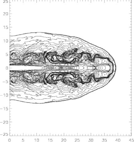
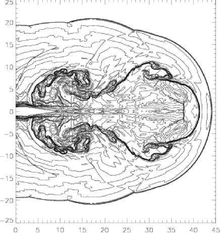
Figure 11: Tadmor’s scheme with PPM reconstruction in a relativistic jet simulation. Rest mass density distribution (in logarithmic scale) at $t=100$ for cylindrical (top panel) and planar (bottom panel) jets.

It is worth commenting on the absence of carbuncle ahead of the bow shock in the simulations reported in Fig. 10. The carbuncle is a numerical pathology well known from blunt body simulations in supersonic gas dynamics, which manifests itself in the form of a small unphysical protuberance in front of the bow shock. In this regard Tadmor’s scheme is able to cleanly resolve (carbuncle-free) the leading bow shock in the jet with an accuracy comparable to that of more sophisticated Godunov-type schemes such as Marquina, and clearly superior to that of Roe-type approximate solvers, which sometimes admit this kind of spurious solution as shown in Donat et al. (1998).

Figure 11 shows the last computed time of our model ($t=100$) in 2D cylindrical and planar coordinates. The morphological elements found in both cases are similar as well as the dynamics governing the jet propagation. The change in geometry is the responsible of the different aspect of the cavity (more elongated in the case of the cylindrical jet).

6 Quantitative comparison

In this section we present a quantitative comparison between Tadmor’s scheme and the HRSC methods based on (approximate) Riemann solvers we have used. To this aim we first compare the numerical and analytic solutions, and show the errors of the various methods for the shock tube problem 3 and problem 6 (propagation of a blast wave with non-zero tangential velocities). We also show in each case the CPU time per numerical cell and iteration (TCI) in order to highlight the computational efficiency of our central scheme.

The results of the comparison are shown in Table 2. This table reports the $L_{1}$ and $L_{\infty}$ norms for the density for Tadmor’s scheme, HLLE, and Roe’s approximate Riemann solvers. Results for both spatial reconstruction procedures (PPM and PHM) are also included. The $L_{1}$ norm errors are computed considering the entire computational domain, while the $L_{\infty}$ errors refer only to the part of the grid where the solution is smooth (i.e. the rarefaction wave). The largest errors occur in the postshock region. From this table we can quantify and confirm the quality of the results shown in the corresponding figures, i.e. that Tadmor’s scheme has an accuracy comparable to that of Riemann solvers based HRSC methods.

Table 2: Errors in the shock tube problems 3 and 6 for HLLE and Roe’s approximate Riemann solvers, and Tadmor’s central scheme using two different third order spatial reconstruction (CFL=0.5 and $N_{x}=400$).

Test	Scheme	$L_{1}$ ($10^{-2}$)		$L_{\infty}$ ($10^{-3}$)
		PPM	PHM	PPM	PHM
Problem 3	HLLE	3.37	2.81	2.87	0.67
	Roe	3.39	2.95	3.44	1.31
	Tadmor	3.41	3.41	2.58	1.04
Problem 6	HLLE	22.0	21.7	3.53	1.20
	Roe	21.7	21.6	2.63	1.20
	Tadmor	25.2	22.4	0.92	2.69

Correspondingly, Table 3 displays the TCI for Tadmor’s scheme and Marquina’s flux formula, which allows us to check their computational efficiency. We note first that when writing the numerical code we did not take special care in optimization issues other than in its most quite apparent aspects. Therefore, the numbers displayed in Table 3 have to be taken as approximate numbers for a standard implementation of a hydrodynamics code, amenable to be improved under code optimization. From this table we can see that Tadmor’s scheme, as expected, consumes less time in doing the calculations than a method based on the characteristic structure of the equations, roughly a factor of 2 for one-dimensional problems, a factor 4 for problem 6 where tangential flow velocities are also involved in the computation, and a factor 3 for a two-dimensional problem (namely, the flat-faced step test).

Table 3: CPU time per numerical cell and iteration for Tadmor’s central scheme and Marquina’s flux formula for the different regimes considered in the text, using third order schemes for the cell reconstruction and time update.

		TCI ($\mu$s)
Case	# Zones	Marquina	Tadmor
1D	400 x 1 x 1	17.0	8.0
1.5D	400 x 1 x 1	32.4	8.8
2D	120 x 40 x 1	72.1	22.7

Some additional comments are in order: firstly, the TCI for Tadmor’s scheme remains essentially unchanged when going from 1D to 1.5D (from 8.0 $\mu$s to 8.8 $\mu$s), which indicates the negligible impact of the computation of the numerical flux in the overall number of operations in the code. Correspondingly, the factor of two difference in Marquina’s flux formula (from 17.0 $\mu$s to 32.4 $\mu$s) is consistent with the large relative weight of the numerical flux step in the overall computation in this algorithm (notice, in particular, that the numerical viscosity matrix changes its dimension from $3\times 3$ to $5\times 5$). Secondly, when going from 1.5D to 2D the TCI in Marquina’s scheme increases by roughly a factor 2.2, while this factor is of the order of 2.5 in the case of Tadmor. A factor two can be easily understood due to the presence of the additional dimension in the code, which implies an additional “sweep” in the corresponding spatial dimension, the cell reconstruction and the numerical flux computation being also computed twice. This factor can be further modified by adding and subtracting two less important factors, namely the access to memory (which is slower as the arrays are larger) and the time update and recovery procedure which are done simultaneously for the two spatial dimensions.

Finally, we show in Table 4 the errors of the density under grid refinement using the discrete $L_{1}$ norm. The results reported in this table correspond to problem 4 at $t=0.4$, and they allow for a comparison of the various schemes (Marquina, HLLE, and Tadmor) and reconstruction procedures (PPM and PHM). The last two columns of the table indicate the convergence rate of the method. As the grid is refined it can be seen how the convergence rate reaches an order of accuracy of roughly one. This is the expected value for problems where discontinuities are present. Furthermore, our result is also in very good agreement with the results of Martí & Müller (1996) where a relativistic extension of PPM was used in conjunction with the exact Riemann solver (see their Table IV).

Table 4: $L_{1}$ norm errors of the density and convergence rate ($r$) under grid refinement for problem 4 at $t=0.4$. Results for three schemes (Marquina, HLLE, and Tadmor) and two reconstruction procedures (PPM and PHM) are shown.

Scheme	N	$L_{1}(10^{-2})$		r
		PPM	PHM	PPM	PHM
Marquina	50	14.8	23.2	—	—
	100	21.0	18.5	-0.50	0.30
	200	16.1	15.1	0.38	0.32
	400	8.99	11.4	0.84	0.41
	800	4.22	7.22	1.09	0.66
	1600	2.22	3.87	0.93	0.90
	3200	1.04	2.06	1.09	0.91
HLLE	50	14.8	23.3	—	—
	100	20.9	17.0	-0.50	0.29
	200	16.1	15.1	0.38	0.33
	400	8.99	11.4	0.84	0.41
	800	4.22	7.22	1.09	0.66
	1600	2.22	3.87	0.93	0.90
	3200	1.04	2.06	1.09	0.91
Tadmor	50	14.7	23.6	—	—
	100	20.7	19.1	-0.49	0.30
	200	16.0	15.2	0.37	0.33
	400	8.94	11.0	0.84	0.47
	800	4.19	7.26	1.09	0.60
	1600	2.21	3.89	0.92	0.90
	3200	1.04	2.07	1.09	0.91

Two important conclusions can be drawn from Table 4: firstly, the transition to the converged solution is faster with PPM than with PHM, especially for grid resolutions finer than $1/400$. The corresponding $L_{1}$ norm errors are also systematically smaller when using the PPM cell-reconstruction routines, roughly a factor of two better than PHM when the number of zones is $\geq 400$. Secondly, both the convergence rate and the errors are pretty much independent of the scheme (Marquina, HLLE, or Tadmor), and irrespective of the grid resolution employed. This result indicates that for a given scheme (either upwind or central) written in conservation form, it is the reconstruction what greatly helps in order to gain accuracy. These conclusions can also be inferred from Fig. 12 which shows the convergence rate in logarithmic scale. It is however important to stress that this result applies to the specific test we have considered (problem 4), for which the wave structure of the solution is particularly simple and the errors are dominated by the presence of discontinuities. It remains to be seen if our conclusion still holds in multidimensional problems involving more complex flows and wave interactions (not necessarily aligned with the computational grid) as those appearing, for instance, when simulating astrophysical jets.

Figure 12: $L_{1}$ norm errors of the density under grid refinement for problem 4 at $t=0.4$. Open (respectively, filled) symbols correspond to results obtained with PPM (respectively, PHM). Results for three schemes (Marquina (squares), HLLE (circles), and Tadmor (triangles)) are shown. For a given grid resolution the accuracy of the solution shows no dependence on the numerical scheme and a strong dependence on the cell-reconstruction.

7 Summary

In this paper we have assessed the validity of a particular finite-difference central scheme in conservation form developed by Kurganov & Tadmor (2000), for the solution of the relativistic hydrodynamic equations. The computations have been restricted to one and two spatial dimensions in flat spacetime. Standard numerical experiments such as shock tubes, the shock reflection test, and the relativistic version of the flat-faced step test have been performed. As an astrophysical application of the central scheme we use we have presented two-dimensional simulations of the propagation of relativistic jets using both Cartesian and cylindrical coordinates. The simulations have shown the capabilities of Tadmor’s scheme to yield satisfactory results, comparable to those obtained by HRSC schemes based on Riemann solvers, even well inside the ultrarelativistic regime. We have proposed to use high-order reconstruction procedures such as those provided by the PPM scheme (Colella & Woodward 1984) and the PHM scheme (Marquina 1999). This is essential to keep the inherent diffusion of central schemes at discontinuities at reasonably low levels.

The novelty of our approach (shared by recent earlier works in the literature (Del Zanna & Bucciantini 2002; Anninos & Fragile 2003)) relies on the absence of Riemann solvers in the solution procedure. Earlier pioneer approaches in the field of relativistic hydrodynamics (Norman & Winkler 1986; Centrella & Wilson 1984) used standard finite-difference schemes in conjunction with artificial viscosity terms to stabilize the solution across discontinuities. Those approaches, however, only succeeded in obtaining accurate results for moderate values of the Lorentz factor ($W\sim 2$). A key feature lacking in those earlier investigations was to write the system of equations and the numerical scheme in conservation form. To the light of our findings and, in addition, to the recent results reported by Anninos & Fragile (2003) where artificial techniques have also been considered in tandem with central schemes, it appears that this was the ultimate reason preventing the extension of the computations to the ultrarelativistic regime.

The use of high-order central schemes for nonlinear hyperbolic systems of conservation laws is increasing in recent years since the seminal work in the second half of the 1980s (Davis 1984; Roe 1984; Yee 1987; Nessyahu & Tadmor 1990). Anile and coworkers (Anile et al. 2000) applied the central scheme SLIC in the context of the time-dependent hydrodynamical semiconductor equations obtaining satisfactory results as well for a system whose characteristic information is not available. In the context of special and general relativistic MHD Koide et al. (1996, 1998) applied a second-order central scheme with nonlinear dissipation developed by Davis (1984) to the study of relativistic extragalactic jets and black hole accretion. This scheme has been lately applied by Mizuno et al. (2003) in general relativistic MHD simulations of the gravitational collapse of a magnetized rotating massive star as a model of gamma ray bursts. Also recently Del Zanna & Bucciantini (2002) and Anninos & Fragile (2003) have assessed two different high-order central schemes in relativistic hydrodynamics, obtaining results as accurate as those of upwind HRSC schemes in standard tests.

The theoretical knowledge of the characteristic information of any hyperbolic system of equations is the key ingredient guiding the construction of HRSC upwind schemes. The different Riemann solvers available in the literature, either exact or approximate (see Martí & Müller (2003) for an up-to-date list in relativistic hydrodynamics), all use in the solution procedure the eigenvalues (characteristic speeds) and/or the eigenvectors (characteristic fields) of the Jacobian matrices of the system. Such solvers provide a minute amount of diffusion across discontinuities while at the same time capture the jumps in a self-consistent way thanks to the implicit use of the Rankine-Hugoniot jump conditions (the so-called shock-capturing property). Having such information available is also very important for the issue of imposing boundary conditions in regions where a priori there could exist some ambiguity. The knowledge of the behavior of the characteristic speeds and, therefore, the local directionality of the flow, greatly simplifies this task.

Needless to say, the alternative of using high-order central schemes as the one discussed here instead of upwind HRSC schemes becomes apparent when the spectral decomposition of the hyperbolic system under consideration is not known. The straightforwardness of a central scheme makes its use very appealing, especially in multi-dimensions where computational efficiency is an issue. Perhaps the most important example in relativistic astrophysics is the system of (general) relativistic magnetohydrodynamic equations. Despite some recent progress has been accomplished in recent years (Romero et al. 1997; Balsara 2001; Komissarov 1999), much more work is certainly needed concerning their solution with HRSC schemes based upon Riemann solvers. Meanwhile, an obvious choice is the use of central schemes.