Pulsar Magnetosphere :
A General Relativistic Treatment

Abstract

A fully general relativistic description of the pulsar magnetosphere is provided. To be more concrete, a study of the pulsar magnetosphere is performed in the context of general relativistic magnetohydrodynamics (MHD) employing the so-called Grad-Shafranov approach. Not surprisingly, the resulting Grad-Shafranov equations and all the other related general relativistic MHD equations turn out to take essentially the same structures as those for the (rotating) black hole magnetosphere. Other different natures between the two cases including the structure of singular surfaces of MHD flows in each magnetosphere are essentially encoded in the different spacetime (metric) contents. In this way, the pulsar and the black hole magnetospheres can be described in an unified fashion. Particularly, the direction of poloidal currents circulating in the neutron star magnetosphere turns out to be the same as that of currents circulating in the black hole magnetosphere which, in turn, leads to the pulsar and the black hole spin-downs via the “magnetic braking”.

I. Introduction

Radio pulsars are perhaps the oldest-known and the least energetic among all of the pulsar categories. The thoretical study of these radio pulsars can be traced back to the 1969 work of Goldreich and Julian gj . In their pioneering work, Goldreich and Julian argued that pulsars, which are thought to be the rotating magnetized neutron stars, must have a magnetosphere with charge-separated plasma. They then demonstrated that an electric force which is much stronger than the gravitational force will be set up along the magnetic field and as a result, the surface charge layer cannot be in dynamical equilibrium. Then there appear steady current flows along the magnetic field lines which are taken to be uniformly rotating since they are firmly rooted in the crystalline crust of the pulsar surface. Although it was rather implicit in their original work, this model for the pulsar electrodynamics does indeed suggest that the luminosity of radio pulsars is due to the loss of their rotational energy (namely the spin-down) and its subsequent conversion into charged particle emission which eventually generates the radiation in the far zone.
Since the pioneering proposals by Gold gold and by Pacini pacini , it has by now been widely accepted that indeed pulsars might be rotating magnetized neutron stars. Nevertheless, since then nearly all the studies on the pulsar electrodynamics have been performed by simply treating the region surrounding the rotating neutron stars as being flat. This simplification may be sufficient just to gain some insight into rough understanding of the origin of the pulsars’ radiation. However, nearly over thirty years have passed of the study of pulsar electrodynamics and it seems to be that now we should treat the problem in a more careful and rigorous manner, namely, in a fully relativistic fashion. Here by relativistic treatment, we mean that we are dealing with the highly self-gravitating compact objects and of course we shall have the rotating neutron stars in mind. Thus we first begin by providing the rationale for treating the vicinity of spinning compact objects such as a rotating neutron star relativistically as a non-trivial curved spacetime. Indeed, we now have a considerable amount of observed data for various species from radio pulsars gj to (anomalous) X-ray pulsars x-ray . Even if we take the oldest-known radio pulsars for example, it is not hard to realize that these objects are compact enough which really should be treated in general relativistic manner. To be more concrete, note that the values of the parameters characterizing typical radio pulsars are ; $r_{0}({\rm radius})\sim 10^{6}(cm)$, $M({\rm mass})\sim 1.4M_{\odot}\sim 2\times 10^{33}(g)$, $\tau({\rm pulsation~{}period})\sim 10^{-3}-1(sec)$, $B({\rm magnetic~{}field~{}strength})\sim 10^{12}(G)$. Thus the Schwarzschild radius (gravitational radius) of a typical radio pulsar is estimated to be $r_{Sch}=2GM_{\odot}/c^{2}\sim 3\times 10^{5}(cm)$ (where $G$ and $c$ denote the Newton’s constant and the speed of light respectively) and hence one ends up with the ratio $r_{0}/r_{Sch}\sim 10^{6}(cm)/3\times 10^{5}(cm)\sim 3$. This simple argument indicates that indeed even the radio pulsar (which is perhaps the least energetic among all of its species) is a highly self-gravitating compact object that needs to be treated relativistically. Once again, the “relativistic” treatment here means that the region surrounding the pulsar, namely the pulsar magnetosphere has to be described by a curved spacetime rather than simply a flat one. Then the question now boils down to ; what would be the relevant metric to describe the vicinity of a rotating neutron star ? Although it does not seem to be well-known, fortunately we have such a metric of the region exterior to slowly-rotating relativistic stars such as neutron stars, white dwarfs and supermassive stars and it is the one constructed long ago by Hartle and Thorne ht . Thus the Hartle-Thorne metric is a stationary axisymmetric solution to the vacuum Einstein equation and in the present work, we shall take this Hartle-Thorne metric as a relevant one to represent the spacetime exterior to slowly-rotating neutron stars.
Having provided the rationale for treating the region surrounding a magnetized rotating neutron star, namely a pulsar fully relativistically as a curved spacetime, we now state our particular objective in this work. In the present work, we would like to study the pulsar magnetosphere in the context of general relativistic magnetohydrodynamics (MHD) by employing the so-called Grad-Shafranov approach gs . We shall consider both the force-free and full MHD situations and accordingly derive the Grad-Shafranov equations for each case, namely, the pulsar equation and the pulsar jet equation respectively. Not surprisingly, then, the resulting Grad-Shafranov equations and all the other related force-free equations or general relativistic MHD equations turn out to take essentially the same structures as those for the (rotating) black hole magnetosphere thorne ; okamoto ; beskin . The essential distinction between the two cases, however, is the spacetime (metric) contents. For the pulsar magnetosphere case, one needs to choose the Hartle-Thorne metric mentioned above whereas for the black hole magnetosphere case, one has to select the Kerr black hole metric kerr . Then as a consequence of this, the singular surfaces of MHD flows in the pulsar magnetosphere and those in the black hole magnetosphere exhibit substantially different nature. In this way, the pulsar and the black hole magnetospheres can be described in an unified fashion. This last point, namely, an unified picture of both the pulsar and the black hole electrodynamics is the key proposal of the present work. There is, however, as strong motive for the present work and it is the uncomfortable current state of affair that there still is no generally accepted standpoint about the structure of pulsar magnetosphere yet beskin2 . To be more concrete, there is yet no complete model for the structure of longitudinal (or poloidal) currents circulating in the neutron star magnetosphere that can provide the solution to the problem, say, of pulsar spin-down (namely, the “braking” of rotating neutron star). As we shall see shortly in the text, a partly satisfying solution to this problem will be provided by treating the region outside a magnetized rotating neutron star as a curved spacetime represented by the Hartle-Thorne metric. Namely it turns out that the structure of space charge-separation and the direction of poloidal current particularly in the force-free limit correctly lead to the magnetic braking torque that spins down the rotating neutron star. This implies that, particularly in the technical aspect, the mechanism of Blandford-Znajek type can be adopted to provide a model which takes the magnetized rotating neutron star as the central engine for some radio, X-ray and even (soft) gamma-ray astrophysical phenomena x-ray just as it has been employed to construct a model taking the rotating black hole as the central engine for active galactic nuclei (AGNs)/quasars bz or even gamma-ray bursts (GRBs) gamma . It, however, seems fair to say that this observation should not be taken as a new discovery but as something that has been expected to some extent. And it is due to the fact that historically the Blandford-Znajek mechanism has been strongly motivated by and thus constructed from the original pulsar model of Goldreich and Julian gj (and perhaps others) with the purpose to apply the main idea to the case of rotating black hole. We also note that there have been extensive critical examinations of the operational aspect of the Blandford-Znajek type mechanism carried out by Punsly punsly1 ; punsly2 .

II. Electrodynamics around the slowly-rotating neutron stars

1. The Hartle-Thorne metric for the region exterior to the slowly-rotating neutron stars
The Hartle-Thorne metric ht is given, in terms of the $(3+1)$-split form, by

$$ds^{2}=-\alpha^{2}dt^{2}+g_{rr}dr^{2}+g_{\theta\theta}d\theta^{2}+g_{\phi\phi}(d\phi+\beta^{\phi}dt)^{2}$$ (1)

where the lapse $\alpha$, (angular) shift $\beta^{\phi}$ and the metric components are

$$\alpha^{2} = \Delta R,~{}~{}~{}\beta^{\phi}=-\omega=-{2J\over r^{3}},$$

$$g_{rr} = {S\over\Delta},~{}~{}~{}g_{\theta\theta}=r^{2}A,~{}~{}~{}g_{\phi\phi}=\varpi^{2}=r^{2}A\sin^{2}\theta,$$ (2)

$$g_{tt} = -[\alpha^{2}-(\beta^{\phi})^{2}g_{\phi\phi}]=-[\Delta R-{4J^{2}\over r^{4}}A\sin^{2}\theta],$$

$$g_{t\phi} = \beta^{\phi}g_{\phi\phi}=-{2J\over r}A\sin^{2}\theta$$

and

$$\Delta = \left(1-{2M\over r}+{2J^{2}\over r^{4}}\right),$$

$$R = \left[1+2\left\{{J^{2}\over Mr^{3}}\left(1+{M\over r}\right)+{5\over 8}{Q-J^{2}/M\over M^{3}}Q^{2}_{2}({r\over M}-1)\right\}P_{2}(\cos\theta)\right],$$ (3)

$$S = \left[1-2\left\{{J^{2}\over Mr^{3}}\left(1-{5M\over r}\right)+{5\over 8}{Q-J^{2}/M\over M^{3}}Q^{2}_{2}({r\over M}-1)\right\}P_{2}(\cos\theta)\right],$$

$$A = 1+2\left[-{J^{2}\over Mr^{3}}\left(1+{2M\over r}\right)\right.$$

$$\left.+{5\over 8}{Q-J^{2}/M\over M^{3}}\left\{{2M\over[r^{2}(1-2M/r)]^{1/2}}Q^{1}_{2}({r\over M}-1)-Q^{2}_{2}({r\over M}-1)\right\}\right]P_{2}(\cos\theta)$$

with $M$, $J$ and $Q$ being the mass, the angular momentum and the mass quadrupole moment of the (slowly) rotating neutron star respectively, $P_{2}(\cos\theta)=(3\cos^{2}\theta-1)/2$ being the Legendre polynomial, and $Q^{m}_{n}$ being the associated Legendre polynomial, namely,

$$Q^{1}_{2}(z) = (z^{2}-1)^{1/2}\left[{3z^{2}-2\over z^{2}-1}-{3\over 2}z\log\left({z+1\over z-1}\right)\right],$$ (4)

$$Q^{2}_{2}(z) = \left[{3\over 2}(z^{2}-1)\log\left({z+1\over z-1}\right)-{3z^{3}-5z\over z^{2}-1}\right]$$

and hence

$$Q^{1}_{2}({r\over M}-1) = {r\over M}\left(1-{2M\over r}\right)^{1/2}\left[{3(r/M)^{2}(1-2M/r)+1\over(r/M)^{2}(1-2M/r)}+{3\over 2}{r\over M}\left(1-{M\over r}\right)\log\left(1-{2M\over r}\right)\right],$$ (5)

$$Q^{2}_{2}({r\over M}-1) = -\left[{3\over 2}\left({r\over M}\right)^{2}\left(1-{2M\over r}\right)\log\left(1-{2M\over r}\right)+{{M/r}(1-M/r)\left\{3(r/M)^{2}(1-2M/r)-2\right\}\over(1-2M/r)}\right].$$

As is well-known, the only known exact metric solution exterior to a rotating object is the Kerr metric kerr . Thus it would be worth clarifying the relation of the Hartle-Thorne metric for slowly-rotating relativistic stars given above to the Kerr metric. As Hartle and Thorne ht pointed out, take the Kerr metric given in Boyer-Lindquist coordinate and expand it to second order in angular velocity (namely, the angular shift $\beta^{\phi}$) followed by a coordinate transformation in the $(r,\theta)$-sector,

$$r\to r\left[1-{a^{2}\over 2r^{2}}\left\{(1+{2M\over r})(1-{M\over r})+\cos^{2}\theta(1-{2M\over r})(1+{3M\over r})\right\}\right],$$

$$\theta\to\theta-a^{2}\cos\theta\sin\theta{1\over 2r^{2}}(1+{2M\over r})$$ (6)

where $a=J/M$. Then one can realize that the resulting expanded Kerr metric coincides with the particular case $Q=J^{2}/M$ (with $Q$ being the mass quadrupole moment of the rotating object) of the Hartle-Thorne metric. Therefore, in general this Hartle-Thorne metric is not a slow-rotation limit of Kerr metric. Rather, the slow-rotation limit of Kerr metric is a special case of this more general Hartle-Thorne metric. As a result, the Hartle-Thorne metric with an arbitrary value of the mass quadrupole moment $Q$ can generally describe a (slowly-rotating) neutron star of any shape (as long as it retains the axisymmetry).
Next, since we shall employ in the present work the Hartle-Thorne metric to represent the spacetime exterior to slowly-rotating neutron stars, we would like to carefully distinguish between the horizon radius of the Hartle-Thorne metric and the actual radius of the neutron stars. Indeed, one of the obvious differences between the black hole case and the neutron star case is the fact that the black hole is characterized by its event horizon while the neutron star has a hard surface. Since this solid surface of a neutron star (which we shall henceforth denote by $r_{0}$) lies outside of its gravitational radius which amounts to the Killing horizon radius of the Hartle-Thorne metric, $r_{H}$ at which $\Delta=(1-2M/r+2J^{2}/r^{4})=0$ in eq.(3), we have $r_{0}>r_{H}$. In the present work, however, we shall never speak of the Killing horizon of the Hartle-Thorne metric as it is an irrelevant quantity playing no physical role.
Now we turn to the choice of an orthonormal tetrad frame. And we shall particularly choose the Zero-Angular-Momentum-Observer (ZAMO) zamo frame which is a sort of fiducial observer (FIDO) frame. Generally speaking, in order to represent a given background geometry, one needs to first choose a coordinate system in which the metric is to be given and next, in order to obtain physical components of a tensor (such as the electric and magnetic field values), one has to select a tetrad frame (in a given coordinate system) to which the tensor components are to be projected. As is well-known, the orthonormal tetrad is a set of four mutually orthogonal unit vectors at each point in a given spacetime which give the directions of the four axes of locally-Minkowskian coordinate system. Such an orthonormal tetrad associated with the Hartle-Thorne metric given above may be chosen as $e^{A}=e^{A}_{\mu}dx^{\mu}=(e^{0},e^{1},e^{2},e^{3})$,

$$e^{0} = \alpha dt=(\Delta R)^{1/2}dt,$$

$$e^{1} = g^{1/2}_{rr}dr=\left({S\over\Delta}\right)^{1/2}dr,$$ (7)

$$e^{2} = g^{1/2}_{\theta\theta}d\theta=rA^{1/2}d\theta,$$

$$e^{3} = g^{1/2}_{\phi\phi}(d\phi+\beta^{\phi}dt)=r\sin\theta A^{1/2}\left[d\phi-{2J\over r^{3}}dt\right]$$

and its dual basis is given by $e_{A}=e^{\mu}_{A}\partial_{\mu}=(e_{0}=e_{(t)},e_{1}=e_{(r)},e_{2}=e_{(\theta)},e_{3}=e_{(\phi)})$,

$$e_{0} = {1\over\alpha}(\partial_{t}-\beta^{\phi}\partial_{\phi})=(\Delta R)^{-1/2}\left[\partial_{t}+\frac{2J}{r^{3}}\partial_{\phi}\right],$$

$$e_{1} = g^{-1/2}_{rr}\partial_{r}=\left(\frac{\Delta}{S}\right)^{1/2}\partial_{r},$$ (8)

$$e_{2} = g^{-1/2}_{\theta\theta}\partial_{\theta}=\frac{1}{rA^{1/2}}\partial_{\theta},$$

$$e_{3} = g^{-1/2}_{\phi\phi}\partial_{\phi}=\frac{1}{rA^{1/2}\sin\theta}\partial_{\phi}.$$

The local, stationary observer at rest in this orthonormal tetrad frame $e^{A}$ has the worldline given by $\{dr=0,~{}d\theta=0,~{}(d\phi+\beta^{\phi}dt)=0\}$ which is orthogonal to spacelike hypersurfaces and has orbital angular velocity given by

$$\omega=\frac{d\phi}{dt}=-\beta^{\phi}=-\frac{g_{t\phi}}{g_{\phi\phi}}=\frac{2J}{r^{3}}.$$ (9)

This is the long-known Lense-Thirring precession lt angular velocity arising due to the “dragging of inertial frame” effect of a stationary axisymmetric spacetime. Indeed, it is straightforward to demonstrate that this orthonormal tetrad observer can be identified with a ZAMO carrying zero intrinsic angular momentum with it. To this end, recall that when a spacetime metric possesses a rotational (azimuthal) isometry, there exists associated rotational Killing field $m^{\mu}=\left(\partial/\partial\phi\right)^{\mu}=\delta^{\mu}_{\phi}$ such that the inner product of it with the tangent (velocity) vector $u^{\mu}=dx^{\mu}/d\tau$ (with $\tau$ denoting the particle’s proper time) of the geodesic of a test particle is constant along the geodesic, i.e.,

$$\tilde{L} = g_{\alpha\beta}m^{\alpha}u^{\beta}=g_{\phi t}m^{\phi}u^{t}+g_{\phi\phi}m^{\phi}u^{\phi}$$ (10)

$$= g_{\phi t}\frac{dt}{d\tau}+g_{\phi\phi}\frac{d\phi}{d\tau}.$$

Now, particularly when the local, stationary observer, which here is taken to be a test particle, carries zero angular momentum, $\tilde{L}=0$, its angular velocity becomes

$$\omega=\frac{d\phi}{dt}=\frac{(d\phi/d\tau)}{(dt/d\tau)}=-\frac{g_{t\phi}}{g_{\phi\phi}}=-\beta^{\phi}$$ (11)

and this confirms the identification of the local observer at rest in this orthonormal tetrad frame given above with a ZAMO.
2. Electrodynamics in curved spacetime : the $(3+1)$-split formalism
Generally speaking, when dealing with the electrodynamics in a curved spacetime, relativists prefer a geometric, covariant, frame-independent approach, representing, say, the electromagnetic field by the field strength tensor $F_{\mu\nu}$. The astrophysicists, on the other hand, would prefer to split this tensor into a 3-dimensional electric field $\mathbf{E}$ and magnetic field $\mathbf{B}$, sacrificing the general covariance of the theory in order to get some insight and achieve a comparison with the familiar flat spacetime electrodynamics. As has been first developed by Macdonald and Thorne thorne , fortunately in stationary curved spacetimes, such as those outside the rotating black holes (the Kerr metric) and the rotating neutron stars (the Hartle-Thorne metric discussed above), one can actually reformulate electrodynamics in terms of an absolute 3-dimensional space and an universal time. And the variables in this reformulation are the familiar electric and magnetic fields $(\mathbf{E},\mathbf{B})$, charge and current density $(\rho_{e},\mathbf{j})$. Indeed, this absolute-space/universal-time formulation of stationary curved spacetimes has deep roots in the so-called $(3+1)$-split formalism of general relativity which had originally been employed in the canonical (or Hamiltonian) quantization of gravity in the 1950s and is nowadays being used in the numerical relativity. Normally, however, such $(3+1)$-split formalism has not been welcome by most relativists due to the arbitrariness of the choice of fiducial reference frame. In the case of stationary black hole/neutron star electrodynamics, however, there is one set of fiducial observers preferred over all others : the Zero-Angular-Momentum-Observer (ZAMO) or Locally-Non-Rotating-Frame (LNRF) observer that we discussed in the above subsection. As is well-known and as we shall see in a moment, when one uses this ZAMO frames one realizes that the $(3+1)$ equations of black hole/neutron star electrodynamics are nearly identical to their counterparts in flat spacetime electrodynamics. For general formulations and more detailed discussions of this $(3+1)$-split formalism we refer the reader to thorne . As such, throughout this work, we shall also employ this space-plus-time formalism in which all the physical quantities are represented by 3-dimensional scalars and vectors as measured by ZAMO, the local observer. For instance, the physical electric and magnetic field components as measured by ZAMO can be read off as the projection of $F_{\mu\nu}$ onto the ZAMO orthonormal tetrad frame (eq.(8)), $F_{AB}=F_{\mu\nu}(e^{\mu}_{A}e^{\nu}_{B})$ and $F_{AB}=\{F_{i0},F_{ij}\}$ where

$$E_{i} = F_{i0},~{}~{}~{}\mathbf{E}=\{E_{i}\},$$

$$B_{i} = \frac{1}{2}\epsilon_{ijk}F^{jk},~{}~{}~{}\mathbf{B}=\{B_{i}\}.$$

III. Pulsar equation - The force-free limit of the Grad-Shafranov equation

The so-called Pulsar equation refers to the force-free limit of the more general Grad-Shafranov equation. The force-free condition essentially amounts to ignoring the (inertial) contributions of the plasma particles when the plasma energy density is assumed to be substantially smaller than that of the magnetic field.
1. Basic equations
(1) Force-free condition
In order eventually to describe the force-free pulsar magnetosphere, we start with the Maxwell equations in the background of the stationary axisymmetric rotating neutron star spacetime thorne

$$\mathbf{\nabla}\cdot\mathbf{E} = 4\pi\rho_{e},~{}~{}~{}\mathbf{\nabla}\cdot\mathbf{B}=0,$$

$$\mathbf{\nabla}\times(\alpha\mathbf{E}) = (\mathbf{B}\cdot\mathbf{\nabla}\omega)\mathbf{m},$$ (12)

$$\mathbf{\nabla}\times(\alpha\mathbf{B}) = 4\pi\alpha\mathbf{j}-(\mathbf{E}\cdot\mathbf{\nabla}\omega)\mathbf{m}$$

where we dropped the terms $\mathcal{L}_{\mathbf{k}}(...)=0$, $\mathcal{L}_{\mathbf{m}}(...)=0$ due to stationarity and axisymmetry. And here $\mathbf{k}=\left(\partial/\partial t\right)$ and $\mathbf{m}=\left(\partial/\partial\phi\right)$ denote the time-translational and the rotational Killing fields associated with the stationarity and the axisymmetry of the Hartle-Thorne metric, respectively and hence $\mathbf{m}\cdot\mathbf{m}=g_{\phi\phi}=\varpi^{2}$ and $\mathbf{m}=\varpi e_{\hat{\phi}}=(g_{\phi\phi})^{1/2}e_{\hat{\phi}}$. Note also that since all the measurements are made by ZAMO, the lapse function $\alpha$ is introduced to convert the ZAMO’s proper time $d\tau$ over to the global time $dt$. Throughout in this section, the force-free condition is assumed to hold, i.e.,

$$\rho_{e}\mathbf{E}+\mathbf{j}\times\mathbf{B}=0,~{}~{}~{}\mathbf{B}=\mathbf{B}_{T}+\mathbf{B}_{P}$$ (13)

which also implies the degeneracy condition $\mathbf{E}\cdot\mathbf{B}=0$. Then this force-free condition indicates that the charged particles are flowing along the magnetic field lines and hence the toroidal (angular) velocity of magnetic field lines (which are frozen into plasma) relative to ZAMO is given by

$$\mathbf{v}_{F}=\left[\frac{\Omega_{F}-\omega}{\alpha}\right]\varpi e_{\hat{\phi}}=\left[\frac{\Omega_{F}-\omega}{\alpha}\right]\mathbf{m}$$ (14)

and then $\mathbf{j}=\mathbf{j}_{T}+\mathbf{j}_{P}$ with $\mathbf{j}_{T}=\rho_{e}\mathbf{v}_{T}$ where $\mathbf{v}_{T}$ consists of $\mathbf{v}_{F}$ given above and the streaming velocity along the toroidal magnetic field lines. Then from the force-free condition above, it follows that

$$\mathbf{E}=\mathbf{E}_{P}=-\frac{1}{\rho_{e}}\mathbf{j}_{T}\times\mathbf{B}_{P}.$$ (15)

(2) Poloidal field components
Consider a magnetic flux through an area $A$ whose boundary is a $\mathbf{m}$-loop,

$$\Psi=\int_{A}\mathbf{B}\cdot d\mathbf{S}.$$ (16)

Then from $d\Psi=\mathbf{\nabla}\Psi\cdot d\mathbf{r}$ and alternatively $d\Psi=\mathbf{B}\cdot(d\mathbf{r}\times 2\pi\varpi e_{\hat{\phi}})=(2\pi\varpi e_{\hat{\phi}}\times\mathbf{B})\cdot d\mathbf{r}$, we get

$$\mathbf{B}_{P}=\frac{\mathbf{\nabla}\Psi\times e_{\hat{\phi}}}{2\pi\varpi}=\frac{\mathbf{\nabla}\Psi\times\mathbf{m}}{2\pi\varpi^{2}}$$ (17)

where we used $\mathbf{m}\cdot\mathbf{m}=g_{\phi\phi}=\varpi^{2}$ and hence

$$\mathbf{E}_{P}=-\mathbf{v}_{F}\times\mathbf{B}_{P}=-\left[\frac{\Omega_{F}-\omega}{2\pi\alpha}\right]\mathbf{\nabla}\Psi.$$ (18)

(3) Poloidal current and toroidal magnetic field
Consider a poloidal current through the same area whose boundary is a $\mathbf{m}$-loop,

$$I=-\int_{A}\alpha\mathbf{j}\cdot d\mathbf{S}$$ (19)

then similarly to the case of poloidal magnetic field, $\mathbf{\nabla}I=-2\pi\varpi e_{\hat{\phi}}\times(\alpha\mathbf{j}_{P})$, we get

$$\alpha\mathbf{j}_{P}=-\frac{\mathbf{\nabla}I\times e_{\hat{\phi}}}{2\pi\varpi}=-\frac{\mathbf{\nabla}I\times\mathbf{m}}{2\pi\varpi^{2}}$$ (20)

and then from eqs(17), (20),

$$\mathbf{j}_{P}=-{1\over\alpha}\frac{dI}{d\Psi}\mathbf{B}_{P}.$$ (21)

Next, consider the Ampere’s law in Maxwell equations

$$\int_{A}\mathbf{\nabla}\times(\alpha\mathbf{B})\cdot d\mathbf{S}=4\pi\int_{A}\alpha\mathbf{j}\cdot d\mathbf{S}-\int_{A}(\mathbf{E}\cdot\mathbf{\nabla}\omega)\mathbf{m}\cdot d\mathbf{S}$$ (22)

which, upon using the Stoke’s theorem and $\mathbf{m}\cdot d\mathbf{S}=\mathbf{m}\cdot(d\mathbf{r}\times 2\pi\mathbf{m})=0$, becomes $2\pi\varpi\alpha|\mathbf{B}_{T}|=-4\pi I$ and hence

$$\mathbf{B}_{T}=-\frac{2I}{\alpha\varpi}e_{\hat{\phi}}=-\frac{2I}{\alpha\varpi^{2}}\mathbf{m}.$$ (23)

Next, using eqs.(12) and (18), one gets the Gauss law equation

$$\rho_{e}={1\over 4\pi}\mathbf{\nabla}\cdot\mathbf{E}_{P}=-{1\over 8\pi^{2}}\mathbf{\nabla}\cdot\left[\frac{\Omega_{F}-\omega}{\alpha}\mathbf{\nabla}\Psi\right]$$ (24)

while the Ampere’s law in eq.(12) yields

$$j_{T} = {1\over 4\pi\alpha}\left\{[\mathbf{\nabla}\times(\alpha\mathbf{B})]_{T}+\varpi(\mathbf{E}\cdot\mathbf{\nabla}\omega)\right\}$$

$$= -\frac{\varpi}{8\pi^{2}\alpha}\left\{\mathbf{\nabla}\cdot\left(\frac{\alpha}{\varpi^{2}}\mathbf{\nabla}\Psi\right)+\left(\frac{\Omega_{F}-\omega}{\alpha}\right)\mathbf{\nabla}\Psi\cdot\mathbf{\nabla}\omega\right\}.$$

Alternatively, by combining eqs.(24) and (25), one gets okamoto

$$\rho_{e} = \left(\frac{\Omega_{F}-\omega}{\alpha}\right)\varpi\left[j_{T}-\frac{1}{4\pi^{2}\varpi}\mathbf{G}\cdot\mathbf{\nabla}\Psi\right]$$ (26)

$${\rm where}~{}~{}~{}\mathbf{G} \equiv {1\over 2}\left[\mathbf{\nabla}\ln\frac{(\Omega_{F}-\omega)\varpi^{2}}{\alpha^{2}}-\frac{(\Omega_{F}-\omega)\varpi^{2}}{\alpha^{2}}\mathbf{\nabla}\omega\right].$$

2. The Grad-Shafranov approach
(1) The Grad-Shafranov equation
Consider the force-free condition $\rho_{e}\mathbf{E}+\mathbf{j}\times\mathbf{B}=0$, and focus on its “poloidal component” equation,

$$-\rho_{e}(\mathbf{v}_{F}\times\mathbf{B})|_{P}+\mathbf{j}\times\mathbf{B}|_{P}=0$$

which yields,

$$-\rho_{e}\left(\frac{\Omega_{F}-\omega}{\alpha}\right)\varpi+j_{T}+{1\over\alpha}\frac{dI}{d\Psi}B_{T}=0.$$ (27)

Now by plugging eqs.(24) and (25) in (27) above and using eq.(23), one arrives at thorne ; okamoto ; beskin

$$\mathbf{\nabla}\cdot\left[\frac{\alpha}{\varpi^{2}}\left\{1-\frac{(\Omega_{F}-\omega)^{2}\varpi^{2}}{\alpha^{2}}\right\}\mathbf{\nabla}\Psi\right]+\frac{(\Omega_{F}-\omega)}{\alpha}\frac{d\Omega_{F}}{d\Psi}|\mathbf{\nabla}\Psi|^{2}+\frac{16\pi^{2}I}{\alpha\varpi^{2}}\frac{dI}{d\Psi}=0$$ (28)

where we assumed a general situation in which the magnetic field lines are, although rooted in the pulsar surface, allowed to have differential rotation. This is the stream equation to determine the field structure of the force-free pulsar magnetosphere.
(2) Electric charge and toroidal current density
From eqs.(26) and (27), one gets the expressions for the charge and toroidal current density okamoto

$$\rho_{e} = \left(\frac{\Omega_{F}-\omega}{4\pi^{2}\alpha}\right)\frac{\frac{8\pi^{2}I}{\alpha^{2}}\frac{dI}{d\Psi}-\mathbf{G}\cdot\mathbf{\nabla}\Psi}{1-\left[\frac{(\Omega_{F}-\omega)\varpi}{\alpha}\right]^{2}},$$ (29)

$$j_{T} = \left(\frac{1}{4\pi^{2}\varpi}\right)\frac{\frac{8\pi^{2}I}{\alpha^{2}}\frac{dI}{d\Psi}-\left[\frac{(\Omega_{F}-\omega)\varpi}{\alpha}\right]^{2}\mathbf{G}\cdot\mathbf{\nabla}\Psi}{1-\left[\frac{(\Omega_{F}-\omega)\varpi}{\alpha}\right]^{2}}.$$

(3) Singular surfaces
In order to distinguish the singular surfaces in the pulsar magnetosphere from those in the (rotating) black hole magnetosphere, we first note the generic distinction between the black hole magnetosphere and the pulsar magnetosphere.
(Black hole magnetosphere)
In this case, the field angular velocity $\Omega_{F}$ is generally in no way connected with the angular velocity of the black hole $\omega(r_{H})=\Omega_{H}$. Indeed, $(\Omega_{F}-\omega)$ changes sign from minus to plus as one moves away from the symmetry axis (recall that $\omega$ denotes the angular velocity of ZAMO).
(Pulsar magnetosphere)
In this case, all the magnetic field lines are firmely rooted in the crystalline crust of the pulsar surface, namely $\Omega_{F}=\Omega_{NS}>\omega$. Thus $(\Omega_{F}-\omega)>0$ namely, since $\Omega_{F}=\Omega_{NS}$, the field angular velocity should be greater than that of ZAMO, $\omega$, everywhere.
To summarize, the spinning black hole rotates the “surrounding” magnetic field lines (generated, say, by currents in the accretions disc) essentially via the frame dragging effect whereas the neutron star rotates “its own dipole” magnetic field lines via its spin motion itself.
We start with the light cylinder. When treating the region exterior to the rotating neutron star as a flat spacetime, there was a single light cylinder at $\varpi=c/\Omega_{F}$. For the case at hand where the region outside of the rotating neutron star is described by a generic curved spacetime, there still is a single light cylinder where the denominators of $\rho_{e}$ and $j_{T}$ vanish, namely at

$$\varpi_{L}=\frac{\alpha c}{(\Omega_{F}-\omega)}.$$ (30)

The only change from the flat spacetime treatment to the curved spacetime one is the notion of relative angular velocity with respect to ZAMO since now all the measurements are made by a local fiducial observer which is ZAMO. Particularly note that in the present case of rotating neutron star, there is only one zero for the denominators of $\rho_{e}$ and $j_{T}$ in eq.(29) instead of two since the field angular velocity should be greater than that of ZAMO, $\omega$ everywhere as we explained above. Certainly, this is in contrast to what happens in the case of rotating black hole magnetosphere when there are two light cylinders where the denominators of $\rho_{e}$ and $j_{T}$ vanish, namely at

$$\varpi_{IL}=\frac{\alpha c}{(\omega-\Omega_{F})},~{}~{}~{}\varpi_{OL}=\frac{\alpha c}{(\Omega_{F}-\omega)}.$$

On the light cylinder, the numerators should vanish in order to have finite $\rho_{e}$ and $j_{T}$ there, i.e.,

$$\frac{4\pi^{2}}{\alpha^{2}}\left(\frac{dI^{2}}{d\Psi}\right)=\mathbf{G}\cdot\mathbf{\nabla}\Psi$$ (31)

which is called the “critical condition”.
We now point out the implication of this distinction between the single light cylinder in the pulsar magnetosphere and the double light cylinders in the black hole magnetosphere.
In the case of rotating black hole magnetosphere, the source or origin of the plasma that will fill the magnetosphere is understood as follows. Note that as one moves from the inner light cylinder toward the outer one, the angular velocity of the magnetic field lines grows, namely $(\Omega_{F}<\omega)\to(\Omega_{F}>\omega)$. Thus somewhere between the two light cylinders, there should be the null surface where

$$\Omega_{F}=\omega~{}~{}~{}{\rm or}~{}~{}~{}\mathbf{v}_{F}=\left[\frac{\Omega_{F}-\omega}{\alpha}\right]\mathbf{m}=0$$ (32)

and hence $\mathbf{E}_{P}=-\mathbf{v}_{F}\times\mathbf{B}_{P}=0$. Then on this null surface,

$$\rho_{e} = -\frac{1}{8\pi^{2}}\mathbf{\nabla}\cdot\left[\frac{\Omega_{F}-\omega}{\alpha}\mathbf{\nabla}\Psi\right]=-\frac{1}{8\pi^{2}\alpha}\mathbf{\nabla}\Psi\cdot\mathbf{\nabla}(\Omega_{F}-\omega),$$

$$j_{T} = \frac{2I}{\alpha^{2}\varpi}\frac{dI}{d\Psi}$$ (33)

and this null surface occurs at $\varpi=\varpi_{N}$ $(\varpi_{IL}<\varpi_{N}<\varpi_{OL})$. Indeed we refer to it as the “null surface” since there must be the spark gaps or the creation zone of nearly neutral plasma situated in its neighborhood. The velocity of the magnetic field lines relative to ZAMO

$$|\mathbf{v}_{F}|=\left[\frac{\Omega_{F}-\omega}{\alpha}\right]\varpi$$

begins to increase from zero at $\varpi=\varpi_{N}$ toward $c$ at $\varpi=\varpi_{OL}$ and then further to infinity as one moves far away from the outer light cylinder where $\omega\to 0$, $\alpha\to 1$. As one moves inward, on the other hand, it begins to increase in magnitude (upon changing sign) from zero at $\varpi=\varpi_{N}$ toward $-c$ at $\varpi=\varpi_{IL}$ and then again further to (negative) infinity at the horizon $r_{H}$ as $\alpha=\alpha(r_{H})=0$ there. Thus ZAMOs in the outer region of the magnetosphere $\varpi>\varpi_{N}$ see the centrifugal “magnetic slingshot wind” blowing outward from the vicinity of the null surface to the acceleration zone and ZAMOs in the inner region of the magnetosphere $\varpi<\varpi_{N}$ see the centrifugal magnetic slingshot wind blowing inward to the horizon.
To summarize, the global structure of the pulsar magnetosphere associated with the singular surfaces is indeed quite different from that of rotating black hole magnetosphere. And it indeed is related to the fact that the black hole is characterized by its event horizon while the neutron star has a hard surface.
3. Poloidal current in the neutron star magnetosphere and the pulsar spin-down
As advertized earlier in the introduction, we now address the issue of pulsar spin-down essentially due to the magnetic braking torque in terms of the structure of longitudinal (or poloidal) currents circulating in the neutron star magnetosphere. To this end, we should start with the space charge-separation in the force-free limit. The presentation that will be given below for the present case of pulsar (which is being treated in a fully general relativistic manner) essentially follows that for the case of rotating black hole okamoto in the context of Blandford-Znajek mechanism.
Recall the definitions for the poloidal magnetic flux (or stream function) $\Psi$ and for the poloidal current $I$ given, respectively, by

$$\Psi=\int_{A}\mathbf{B}\cdot d\mathbf{S},~{}~{}~{}I=-\int_{A}\alpha\mathbf{j}\cdot d\mathbf{S}.$$

First, we consider the case when the angular momentum $J_{NS}$ and the (asymptotic) direction of the magnetic field $B$ are parallel. We begin by noting that the magnetic flux (and $\mathbf{B}$) is defined to be positive when it directs upward while the poloidal current is defined to be positive when it directs downward. Normally one imposes the condition of no net loss of charge from the pulsar. This amounts to demanding that the net current flowing into and out of the neutron star surface $A_{NS}$ vanishes, namely

$$\int_{A_{NS}}\alpha\mathbf{j}\cdot d\mathbf{S}=\int_{A_{NS}}\left(-\frac{dI}{d\Psi}\right)\mathbf{B}_{P}\cdot d\mathbf{S}=-[I(\Psi_{eq})-I(\Psi_{0})]=0$$ (34)

where we used $\mathbf{j}=\mathbf{j}_{T}+\mathbf{j}_{P}$, $\mathbf{j}_{T}\cdot d\mathbf{S}=0$ and $d\Psi=\mathbf{B}\cdot d\mathbf{S}=\mathbf{B}_{P}\cdot d\mathbf{S}$. And for the expression for the poloidal current density $\mathbf{j}_{P}$, we used eq.(21). Here, the surface integral is taken only over the (nothern) hemisphere of the neutron star surface from the (north) pole where $\Psi=\Psi_{0}$ to the equator where $\Psi=\Psi_{eq}$ as the pulsar’s intrinsic dipole moment would generate dipole magnetic fields. This condition indeed implies the presence of some “critical” magnetic surface $\Psi=\Psi_{c}$ such that

$$\frac{dI}{d\Psi}=\left\{\begin{array}[]{ll}>0&\hbox{({\rm for} $\Psi_{0}<\Psi<\Psi_{c}$) : ~{}{\rm Region ~{}I}, }\\ 0&\hbox{({\rm for} $\Psi=\Psi_{c}$),}\\ <0&\hbox{({\rm for} $\Psi_{c}<\Psi<\Psi_{eq}$) : ~{}{\rm Region ~{}II}.}\\ \end{array}\right.$$ (38)

Then one can realize from eqs.(35) and (21) that the electric current flows inwardly along the magnetic field lines for $\Psi_{0}<\Psi<\Psi_{c}$ from the acceleration region to the neutron star surface while it flows outwardly for $\Psi_{c}<\Psi<\Psi_{eq}$ from the surface to the acceleration region. And on the critical magnetic surface $\Psi=\Psi_{c}$, the net current is zero (i.e., inflowing current $=$ outflowing current) but the charge density there may not be exactly zero and hence the critical magnetic surface may not serve as exactly a “charge-separating” surface. This point can be envisaged from the expression for the charge density $\rho_{e}$ in eq.(29) where one can notice that $dI/d\Psi$ is zero but $\mathbf{G}\cdot\mathbf{\nabla}\Psi$ is not necessarily zero along $\Psi=\Psi_{c}$. Indeed, this last quantity can roughly be identified with the vertical component of the magnetic field (i.e., $B_{z}$). In the Goldreich-Julian (GJ) model gj of purely charge-separated magnetosphere, the critical magnetic surface has been defined as the one on which $B_{z}=0$ all the way. In our model of pulsar magnetosphere with infinite supply of quasi-neutral plasma, on the other hand, it is being defined as the one on which $dI/d\Psi=0$. As such, generally the critical magnetic surfaces in the two models may not coincide and as a result, in our model the critical magnetic surface may not act as precisely a charge-separating surface. The origin of different predictions of these two models shall be discussed in detail later on in the subsection 5 of the present section.
Next, in the case when the angular momentum $J_{NS}$ and the (asymptotic) direction of the magnetic field $B$ are antiparallel, all the quantities involved would carry flipped signs, namely

$$\frac{dI}{d\Psi}=\left\{\begin{array}[]{ll}<0&\hbox{({\rm for} $\Psi_{0}<\Psi<\Psi_{c}$) : ~{}{\rm Region ~{}I}, }\\ 0&\hbox{({\rm for} $\Psi=\Psi_{c}$),}\\ >0&\hbox{({\rm for} $\Psi_{c}<\Psi<\Psi_{eq}$) : ~{}{\rm Region ~{}II}.}\\ \end{array}\right.$$ (42)

This second case when $J_{NS}$ (or $J_{BH}$ that we shall also discuss shortly) and $B$ are antiparallel is indeed likely to happen. First for the pulsar case, its spin angular momentum $J_{NS}$ and its intrinsic magnetic dipole moment may well be aligned and pointing the opposite directions at the same time to yield the antiparallel configuration of this type. For the rotating black hole case, on the other hand, consider, for instance, that the poloidal magnetic fields come from the toroidal currents in the accretion disc around the hole. Clearly, the hole and the disc would be corotating but if the excess charge is due to that of ions, the spin of the hole $J_{BH}$ and the magnetic field would be parallel whereas if it is due to that of electrons, the two would be antiparallel instead.
With this preparation, we now turn to the determination of the structure of space charge-separation and the direction of the poloidal current in the neutron star (and the rotating black hole for comparison) magnetosphere. Consider the charge density in the neutron star magnetosphere given earlier in eq.(29) (note that its structure remains the same even in the rotating black hole magnetosphere except that the associated spacetime metric content is distinct between the two cases),

$$\rho_{e}=\left(\frac{\Omega_{F}-\omega}{4\pi^{2}\alpha}\right)\frac{\left(\frac{8\pi^{2}I}{\alpha^{2}}\right)\frac{dI}{d\Psi}-\mathbf{G}\cdot\mathbf{\nabla}\Psi}{\left[1-\frac{(\Omega_{F}-\omega)\varpi}{\alpha}\right]\left[1+\frac{(\Omega_{F}-\omega)\varpi}{\alpha}\right]}.$$ (43)

Now using this expression for the charge density along with eqs.(35) and (36), one can, in principle determine the sign of the separated charges in different domains of the neutron star magnetosphere. The directions of poloidal current densities are determined using basically the eq.(21) accordingly. The resulting charge-separation and the poloidal current direction are depicted in FIG.1.

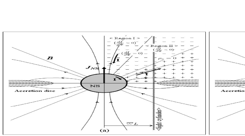
Figure 1:  Pulsar magnetosphere - a general relativistic treatment. The presence of accretion disc disc here is not mandatory but is assumed for parallel comparison with the case of black hole magnetosphere. The star’s intrinsic dipole moments are not drawn in the figures.
(a) When $J_{NS}$ and $B$ are parallel, (b) when $J_{NS}$ and $B$ are antiparallel.

It is indeed quite instructive to compare the present case of pulsar magnetosphere structure with that of rotating black hole magnetosphere structure. The latter had been studied in detail in the literature bz ; thorne ; tomimatsu ; okamoto ; beskin and here in the present work, we have elaborated on it by further considering the case when the spin of the hole and the (asymptotic) direction of the magnetic field are antiparallel - see FIG.2.
In practice, however, determining the sign of the separated charges in different domains of the neutron star/black hole magnetosphere using eqs.(35), (36) and (37) is by no means a straightforward job. Technically, the associated difficulty arises from the fact that we need to figure out which term, between $|(8\pi^{2}I/\alpha^{2})(dI/d\Psi)|$ and $|\mathbf{G}\cdot\mathbf{\nabla}\Psi|$ in the numerator of eq.(37), is greater than the other in different domains of the magnetosphere. By contrast, the determination of the structure of charge separation (i.e., the sign of separated charges) in the GJ model (but only inside the light cylinder) that we shall discuss shortly and summarized in FIG.3 using eq.(38) below is rather straightforward. Fortunately, however, there is a guiding principle that allows us to determine the sign of separated charges in different domains with confidence. And that is just the insightful realization that the different domains of the magnetosphere around the compact object such as the rotating neutron star or black hole should rotate in the same direction as the compact object itself (“corotation”) if they rotate faster than ZAMO, the local inertial observer carryng out all the observations, whereas they should rotate in the opposite direction (“counter-rotation”) provided they rotate slower than ZAMO. In order to work out this guiding principle and determine the structure of charge separation as a result, we begin by defining the angular momentum of the magnetosphere. The pulsar magnetosphere consists of the poloidal magnetic field generated essentially by the intrinsic dipole moment of the neutron star and the poloidal electric field generated both by the toroidal current-poloidal magnetic field in the force-free limit (see eqs.(14) and (18)) and by the separated space charge. And particularly these two sources of the poloidal electric field are closely related since the toroidal current arises as a result of the angular motion of the poloidal magnetic field lines (being dragged along by the spin of the neutron star) along which the plasma flows (in the force-free limit). Therefore if one can determine the direction of the poloidal electric field, the structure of charge separation can be determined accordingly. Besides, since the motion of the plasma eventually generates the poloidal electric field, the angular momentum of the magnetosphere can be defined in terms of its poloidal electromagnetic field. In general, the angular momentum of an electromagnetic field is defined by $\mathbf{J}_{em}=\int d^{3}x[\mathbf{r}\times(\mathbf{E}_{P}\times\mathbf{B}_{P})]$. Thus we only need to determine the direction of this poloidal electric field $\mathbf{E}_{P}$ (for a given poloidal dipole magnetic field $\mathbf{B}_{P}$) that leads to either corotation or counter-rotation of the different domains of the magnetosphere (as measured by ZAMO, the local inertial observer) with the rotating neutron star/black hole, i.e., $\mathbf{J}_{em}\sim\pm\mathbf{J}_{NS,BH}$. This is how the structure of charge separation in different domains of the pulsar magnetosphere summarized in FIG.1 and that of the black hole magnetosphere summarized in FIG2. have been actually fixed. It is worthy of note that for the case of pulsar magnetosphere, the sign of separated charges in different domains such determined is the same as that in the original GJ model that we shall turn to in a moment except that now for our force-free treatment, it can be extrapolated outside the light cylinder. Next, for the case of black hole magnetosphere, the structure of charge separation such determined turns out to be exactly the same again as the result derived by Okamoto okamoto some time ago via different reasoning.

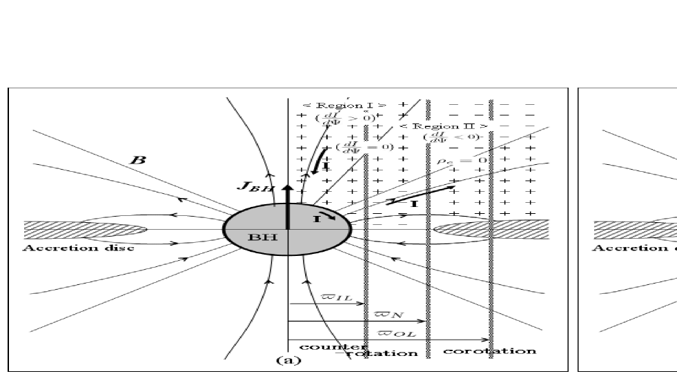
Figure 2:  Rotating black hole magnetosphere. Although the critical magnetic surfaces have been sketched more or less as straight lines in these figures, they would in fact be curved in actual situation.
(a) When $J_{BH}$ and $B$ are parallel, (b) when $J_{BH}$ and $B$ are antiparallel.

Then to summarize, it is not surprising (since it has been expected to some extent) but still interesting to realize that the structure of magnetosphere of the pulsar and the rotating black hole are not quite the same let alone the different structure of singular surfaces that we stressed earlier. If we emphasize it once again, this difference can be attributed to the fact that all the magnetic field lines are firmely rooted in the crystalline crust of the pulsar surface and hence $\Omega_{F}=\Omega_{NS}>\omega$ namely, the field angular velocity is greater than that of ZAMO, $\omega$, everywhere. Consequently, to the ZAMO of rotating neutron star, the whole pulsar magnetosphere looks corotating and thus the resulting direction of the poloidal electric field eventually determines the structure of space charge separation as given in FIG.1. In the black hole case, however, the field angular velocity $\Omega_{F}$ is generally in no way connected with the angular velocity of the black hole $\omega(r_{H})=\Omega_{H}$. Indeed, $(\Omega_{F}-\omega)$ changes sign from minus to plus as one moves away from the symmetry axis (recall that $\omega$ denotes the angular velocity of ZAMO). Namely, inside the “null surface” that we discussed earlier in subsection 2, ZAMO rotates faster than the magnetic field lines (and hence than the inner part of the magnetosphere) while outside of it, ZAMO rotates slower than the magnetic field lines (and thus the outer part of the magnetosphere). As a result, to the ZAMO of rotating black hole, the part of black hole magnetosphere outside the null surface looks corotating whereas its part inside the null surface appears to counter-rotating. From this one can realize the directions of the poloidal electric fields which, in turn, determines the structure of space charge separation as given in FIG.2. And for both pulsar and rotating black hole cases, it is rather straightforward to see that the structure of charge-separation and the direction of longitudinal (or poloidal) current (denoted in the figures by $I$) circulating in the magnetospheres actually lead to the magnetic braking torques, namely the Lorentz torques $\mathbf{N}=\int_{A_{NS(H)}}[\mathbf{r}\times(\mathbf{j}_{P}\times\mathbf{B})]d|\mathbf{S}|$, that spin down the rotating neutron star and the black hole as it is always directed opposite to the spins regardless of whether the spin and the (asymptotic) direction of the magnetic field are parallel or ntiparallel. Here, the surface area $A_{NS(H)}$ over which the integral of the non-vanishing Lorentz torque density is to be taken might need some careful clarification. For the case of rotating neutron star, this area obviously should be its surface where the poloidal current crosses the magnetic field lines and hence generates non-vanishing braking torque. For the case of black hole, however, the nature of this area might seem quite ambiguous but our suggestion here is to invoke the notion of “stretched horizon” as an incarnation of the so-called “membrane paradigm” membrane . Indeed, the philosophy that underlies the membrane paradigm is an attempt to have an intuitive picture of Blandford-Znajek mechanism by first assuming the appearance of stretched horizon (just outside the event horizon) and then introducing (fictitious) surface charge and current density on it. Then one of the most intriguing consequences of such assumption is that if we choose to do so, the (stretched) horizon behaves as if it is a conductor with finite resistivity. To be more specific, since there are now both current and resistivity on the horizon, one might naturally wonder what would happen to the Joule heat generated when those surface currents work against the resistance and how it would be related to the electromagnetic energy going down the hole through the horizon. Indeed, Znajek and independently Damour zd provided a simple and natural answer to this question. Namely, they showed in a consistent and elegant manner that the total electromagnetic energy flux (i.e., the Poynting flux) into the rotating Kerr hole through the horizon is indeed precisely the same as the amount of Joule heat produced by the surface currents when they work against the surface resistivity of $4\pi$. Therefore, motivated and encouraged by these ground works for the advent of the membrane paradigm, here we also assume that the surface area over which the integral of the non-vanishing Lorentz torque is to be taken is just this stretched horizon with surface current. Then the real poloidal current in the black hole magnetosphere and this surface current on the horizon together are supposed to complete the circuit.
Now to summarize, this unified picture can be thought of as a satisfying solution to both the magnetized rotating neutron star interpretation of radio/X-ray pulsars x-ray and the rotating supermassive black hole interpretation of AGNs/quasars bz or even GRBs gamma .
It is, however, the following point that is of great interest and has been the strong motive for the present study. And it is the difference in the nature of the origin/source of charges which get separated in the domains of the magnetosphere and of the resulting poloidal currents between the two pulsar models - ours and that of Goldreich-Julian’s. It goes as follows.
First, the original GJ model can be thought of as the purely charge-separated solution in which only one charge species can be assigned at a given point in space. As a result, the poloidal current in this charge-separated solution is directly proportional to charge density. Now, the origin/source of charges in this GJ model is basically the surface of the pulsar itself and the poloidal current flows only until these charges get separated (by the strong local electric field near the surface of the star) and then reach the equilibrium GJ charge density given by

$$\rho^{GJ}_{e}=-\frac{1}{2\pi c}\frac{\mathbf{B}\cdot\mathbf{\Omega}}{1-\left(\frac{\Omega r}{c}\right)^{2}\sin^{2}\theta}=-\frac{\Omega}{2\pi c}\frac{B_{z}}{1-\left(\frac{\varpi}{\varpi_{L}}\right)^{2}}$$ (44)

where we restored the speed of light $c$ and $\Omega$ denotes the angular velocity of the pulsar. Working with this expression for the pulsar charge density, the resulting charge-separation can be determined as depicted in FIG.3. By contrast, our force-free (and fully general relativistic) model may be referred to as the solution of quasi-neutral plasma in which two species of charges can coexist at a given point in space while allowing for still non-zero net space charge density. And non-trivial poloidal current can still exist as it can be defined in terms of the difference in velocities between the two charge species. Then the origin/source of charges in this force-free treatment is mainly the pair creation due to strong electromagnetic field in space which provides infinite supply of ample plasma and hence the continuous flow of poloidal current without end. This difference in the nature of charges and the resulting poloidal currents between the two model is indeed the key to understand why our force-free and general relativistic treatment of the pulsar magnetosphere presents more self-consistent and hence satisfying view of the pulsar spin-down mechanism in the sense that it is consistent with the mechanism of Blandford and Znajek bz employing the rotating black hole magnetosphere. This essential difference between the two pulsar models, however, do not necessarily mean that our force-free and general relativistic treatment is able to provide a successful mechanism for pulsar spin-down in terms of the magnetic braking torque while Goldreich-Julian’s original but non-general relativistic (GR) one fails to do so. And obviously in order to be convinced that both of the two models can successfully provide the mechanism for the pulsar’s magnetic spin-down, one needs to demonstrate that the directions of poloidal currents particularly at the surface of the neutron star are indeed the same correctly leading to the magnetic braking torque that we discussed earlier. Thus in the following, this last point shall be addressed. Indeed, the directions of the poloidal current (that closes globally in the magnetosphere) are defined differently in the two models. First in our force-free treatment, the direction of the poloidal current and the structure of the charge densities given in eqs.(21) and (29) respectively are determined simultaneously via the behavior of the quantity $(dI/d\Psi)$ as given in eqs.(35) or (36) just as it was the case with the rotating black hole magnetosphere thorne ; okamoto . Namely, one is not determined as a result of the other. Of course, this is because the continuous supply of ample plasma is assumed in our treatment as discussed above. And as depicted in FIG.1, the direction of poloidal current such determined particularly at the surface of the star correctly leads to the magnetic braking torque directed opposite to the star’s angular momentum.
In the original model of Goldreich-Julian’s gj ; punsly2 , on the other hand, the structure (i.e., the sign) of charge density is actually determined as a result of the direction of the poloidal current. That is, the strong local electric field near the surface of the neutron star first determines the direction of local poloidal current (i.e., the flow of local charge carriers) which, in turn, determines the sign of local charges in a given domain of space. To be more specific, Goldreich and Julian began their analysis by assuming that the neutron star with an aligned dipole magnetic field is surrounded first by vacuum. Then the longitudinal electric field at the neutron star surface turns out to have component parallel to the poloidal magnetic field given by $E_{||}\sim-\cos^{3}\theta$ and particularly at the equator the vacuum electric field is directed radially outward. Thus in the polar region, the vacuum longitudinal electric field drives a current towards the star (by pulling space ions if present or by ripping electrons off the pulsar surface) while at the equator it drives current away from the star (by pulling space electrons if present or by ripping ions off the surface). In this way, the vacuum longitudinal electric field causes charge emission, i.e., the flow of the poloidal current, only until the magnetosphere is filled with plasma with the charge density being given by the Goldreich-Julian’s equilibrium value given in eq.(38). Namely, the poloidal current cannot flow without end because once the charges get accumulated up to GJ’s equilibrium value in eq.(38), the emission of charges becomes electrostatically unfavorable. And if, particularly in the particle acceleration region, there appears the difference between the local plasma charge density and the equilibrium Goldreich-Julian density $\rho^{GJ}_{e}$ given in eq.(38), the longitudinal electric field arises and as a result, the plasma in the magnetosphere would be streaming out along open magnetic field lines past the light cylinder as a centrifugally slung, relativistic wind leading eventually to the observed radio emission. Note that if the current driven by the vacuum longitudinal electric field can close in a global current system, particularly the direction of the current flowing on the stellar surface again would exert the correct magnetic braking or spin-down torque on the neutron star. In this non-GR Goldreich-Julian model, therefore, the charge-separation depicted in FIG.3 does not really conflict with the spin-down process as the direction of the poloidal current is indeed the same as that of our force-free treatment discussed above correctly leading to essentially the same magnetic braking torque. Thus to summarize, regardless of the difference in the origin/source of the space charges and in the definition of the direction of poloidal current, both the Goldreich-Julian’s original model and our present force-free treatment provide the working mechanism for magnetic pulsar spin-down. Nevertheless, we would like to stress again that there indeed is a more desirable feature in our treatment that distinguishes it from the original model of Goldreich and Julian’s. And it is the fact that the force-free and fully general relativistic treatment of the problem of pulsar magnetosphere presented in this work appears to provide much upgraded and closer view of the pulsar spin-down mechanism in the sense that it is consistent with the mechanism of Blandford and Znajek bz ; thorne ; tomimatsu ; okamoto ; beskin employing the rotating black hole magnetosphere.
Thus far, we have been interested in the comparison between our force-free and general relativistic model and the Goldreich-Julian’s non-GR model of pulsar magnetosphere. And it has been realized that the main differences between the two arise not from the GR effect but from the different nature and source of the charges. Now this realization leads us to turn to another relevant comparison. That is, it seems equally relevant to consider the comparison of our force-free and general relativistic treatment with a force-free but non-GR treatment of pulsar magnetosphere and see if there is actually something generic in fully general relativistic treatment of the pulsar electrodynamics. Indeed such force-free but non-GR study of pulsar magnetosphere has been perfomed some time ago by Okamoto okamoto2 and by Contopoulos, Kazanas and Fendt ckf . Later on in the subsection 5 of the present section, the rigorous comparison of our present treatment with this second class of study shall be carried out and if we mention the essential result in advance, as far as the pulsar electrodynamics goes, the GR treatment does not seem to have any generic effect other than the stereotypical complications and elaborations such as the large redshift near the neutron star’s surface and the frame-dragging effect and hence the quest for the introduction of ZAMO, the local inertial observer carrying out the actual observations. Indeed, the existence of and the observations by ZAMO is a non-trivial deviation from non-GR treatment of the pulsar electrodynamics since it is the strong electric field felt by ZAMO that actually renders the pair creation of charges via the so-called Schwinger process work mt . Recall that our model of pulsar magnetosphere depends, for the source of ample supply of quasi-neutral plasma, heavily on the pair production of charges in space.
To summarize, it has been quite uneasy to accept that the two relativistic spinning compact objects of nearly the same species, the neutron star (i.e., pulsar) (based on the Goldreich-Julian model) and the black hole (based on, say, the Blandford-Znajek model) have generically different structures of magnetospheres. And in our force-free and general relativistic pulsar model, we realized that it shares the same structure of singular surfaces of flows with that of original Goldreich-Julian model on the one hand and shares essentially the same structures of charge-separation and the poloidal current with those of rotating black hole bz ; okamoto on the other.

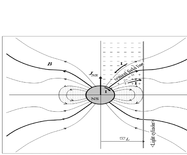
Figure 3:  Pulsar magnetosphere - the Goldreich-Julian’s aligned rotator model.

4. The energy and the angular momentum flux
In the above, we showed, in terms of the space charge-separation structure of the pulsar magnetosphere, that in the force-free case the longitudinal (or poloidal) currents circulating in the neutron star magnetosphere leads to the magnetic braking torque that actually spins it down in a similar manner to the case with the Blandford-Znajek mechanism for the extraction of rotational energy from Kerr black holes. In this subsection, we shall demonstrate, in terms of the energy and the angular momentum flux at the surface of the neutron star, that this argument does indeed hold true. The general expression for the redshifted energy flux $\mathbf{S}_{E}$ and the angular momentum flux about the axis of rotation $\mathbf{S}_{L}$ are given respectively by thorne

$$\mathbf{S}_{E} = {1\over 4\pi}[\alpha(\mathbf{E}\times\mathbf{B})-\omega(\mathbf{E}\cdot\mathbf{m})\mathbf{E}-\omega(\mathbf{B}\cdot\mathbf{m})\mathbf{B}+{1\over 2}\omega(\mathbf{E}^{2}+\mathbf{B}^{2})\mathbf{m}],$$

$$\mathbf{S}_{L} = {1\over 4\pi}[-(\mathbf{E}\cdot\mathbf{m})\mathbf{E}-(\mathbf{B}\cdot\mathbf{m})\mathbf{B}+{1\over 2}(\mathbf{E}^{2}+\mathbf{B}^{2})\mathbf{m}].$$ (45)

Since the toroidal component of the fluxes are irrelevant, we only need to consider the poloidal components

$$\mathbf{S}^{P}_{L} = -{\varpi\over 4\pi}|\mathbf{B}_{T}|\mathbf{B}_{P}={I\over 2\pi\alpha}\mathbf{B}_{P},$$ (46)

$$\mathbf{S}^{P}_{E} = {\alpha\over 4\pi}\mathbf{E}_{P}\times\mathbf{B}_{T}+\omega\mathbf{S}^{P}_{L}={I\over 2\pi}\left(\frac{\omega}{\alpha}\mathbf{B}_{P}-\frac{1}{\varpi^{2}}\mathbf{E}_{P}\times\mathbf{m}\right).$$

Thus, at the neutron star surface where $\alpha=\alpha(r_{s})\neq 0$,

$$-\mathbf{S}_{L}\cdot\mathbf{n}\to\frac{dJ}{d\Sigma_{s}dt} = -{I\over 2\pi\alpha}B_{\perp}=-\frac{I}{4\pi^{2}\alpha\varpi}(\mathbf{\nabla}\Psi\times e_{\hat{\phi}})\cdot\mathbf{n},$$ (47)

$$-\mathbf{S}_{E}\cdot\mathbf{n}\to\frac{dM}{d\Sigma_{s}dt} = -{I\over 2\pi}\left[\frac{\omega}{\alpha}B_{\perp}-\frac{1}{\varpi}(\mathbf{E}_{P}\times e_{\hat{\phi}})\cdot\mathbf{n}\right]$$

$$= -{I\over 2\pi\alpha}\Omega_{F}B_{\perp}=\Omega_{F}\frac{dJ}{d\Sigma_{s}dt}$$

where $\mathbf{n}$ denotes the unit vector outer normal to the neutron star surface. Now note that when the spin $J$ of the rotating neutron star and the magnetic field $\mathbf{B}$ are parallel, $B_{\perp}>0$, $I>0$ whereas when $J$ and $\mathbf{B}$ are antiparallel, $B_{\perp}<0$, $I<0$ due to their definitions eqs.(16) and (19). Namely, the magnetic flux (and $B$) is defined to be positive/negative when it directs upward/downward while the poloidal current is defined to be positive/negative when it directs downward/upward as we noted earlier. Thus one always has $IB_{\perp}>0$, and hence from eq.(41) above, we always have

$$-\mathbf{S}_{L}\cdot\mathbf{n} = -{I\over 2\pi\alpha}B_{\perp}<0,$$ (48)

$$-\mathbf{S}_{E}\cdot\mathbf{n} = -{I\over 2\pi\alpha}\Omega_{F}B_{\perp}<0.$$

Since the angular momentum and the energy flux going into the neutron star surface are all negative, this means that the rotating neutron star (i.e., the pulsar) experiences magnetic braking torque, namely spins-down and as a result, always loses part of its rotational energy (at the surface).
5. Limit of vanishing general relativistic effects
In earlier subsections, we have studied the detailed comparison between our force-free and general relativistic model and the Goldreich-Julian’s non-GR model of pulsar magnetosphere. It then has been argued that the main differences between the two arise not from the GR effect but from the different nature and source of the charges. This could be checked in a rigorous manner if we erase the GR content in our force-free treatment of the pulsar magnetosphere and see if these differences still remain. We also have turned to another equally relevant comparison. Namely, we have considered the comparison of our force-free and general relativistic treatment with a force-free but non-GR treatment of pulsar magnetosphere to see whether there is actually something generic in fully general relativistic treatment of the pulsar electrodynamics. Again, such a comparison would be made explicit if the GR component in our treatment is washed out. Besides, such force-free but non-GR study of pulsar magnetosphere has been perfomed in the literature okamoto2 ; ckf and hence the result of the comparison can be directly tested. Therefore in this subsection, we shall reconsider our force-free and general relativistic model and take its particular limit of vanishing GR content for these purposes.
Evidently, taking the limit of vanishing GR content would amount to replacing the curved Hartle-Thorne spacetime exterior to the rotating neutron star with the flat spacetime while maintaining the force-free nature of pulsar electrodynamics. And technically, this is equivalent to setting all the parameters associated with the non-trivial curved spacetime structure, i.e., the mass $M$, angular momentum $J$ and the mass quadrupole moment $Q$ in the Hartle-Thorne metric for the neutron star, to zero in all the equations of the pulsar electrodynamics presented in the subsections 1 and 2 above.
In the limit of vanishing GR content, apparently the exterior spacetime is the flat Minkowski one and in the following we shall take the cylindrical coordinates $(t,R,\phi,z)$ in which the Minkowski metric is given by

$$ds^{2}=-dt^{2}+dR^{2}+R^{2}d\phi^{2}+dz^{2}.$$ (49)

Then the role played by proper distance from the axis of (neutron star’s) rotation $\varpi$ that has been employed thus far in the general relativistic treatment shall henceforth be taken over by the radial coordinate $R$. Next, we start with the Maxwell equations in this flat spacetime

$$\mathbf{\nabla}\cdot\mathbf{E} = 4\pi\rho_{e},~{}~{}~{}\mathbf{\nabla}\cdot\mathbf{B}=0,$$

$$\mathbf{\nabla}\times\mathbf{E} = 0,~{}~{}~{}\mathbf{\nabla}\times\mathbf{B}=4\pi\mathbf{j}$$ (50)

where we dropped the terms $\partial(...)/\partial t=0$, $\partial(...)/\partial\phi=0$ due to stationarity and axisymmetry. Next, throughout, the force-free condition is still assumed to hold, i.e.,

$$\rho_{e}\mathbf{E}+\mathbf{j}\times\mathbf{B}=0,~{}~{}~{}\mathbf{B}=\mathbf{B}_{T}+\mathbf{B}_{P}$$ (51)

which also implies $\mathbf{E}\cdot\mathbf{B}=0$. Then this force-free condition indicates that the charged particles are sliding along the magnetic field lines and hence the toroidal (angular) velocity of magnetic field lines (which are frozen into plasma) is given by

$$\mathbf{v}_{F}=R\Omega_{F}e_{\hat{\phi}}=\Omega_{F}\mathbf{m}$$ (52)

and then $\mathbf{j}=\mathbf{j}_{T}+\mathbf{j}_{P}$ with $\mathbf{j}_{T}=\rho_{e}\mathbf{v}_{T}$ where $\mathbf{v}_{T}$ consists of $\mathbf{v}_{F}$ given above and the streaming velocity along the toroidal magnetic field lines. Here, again $\mathbf{m}=Re_{\hat{\phi}}=(g_{\phi\phi})^{1/2}e_{\hat{\phi}}$. Then from the force-free condition above, it follows that

$$\mathbf{E}=\mathbf{E}_{P}=-\frac{1}{\rho_{e}}\mathbf{j}_{T}\times\mathbf{B}_{P}.$$ (53)

We have established the force-free condition and based on this, we can now derive all the force-free pulsar electrodymanics equations. First we consider the poloidal field components.
As before, a magnetic flux through an area $A$ whose boundary is a $\mathbf{m}$-loop is given by

$$\Psi=\int_{A}\mathbf{B}\cdot d\mathbf{S}.$$ (54)

Then from $d\Psi=\mathbf{\nabla}\Psi\cdot d\mathbf{r}$ and alternatively $d\Psi=\mathbf{B}\cdot(d\mathbf{r}\times 2\pi Re_{\hat{\phi}})=(2\pi Re_{\hat{\phi}}\times\mathbf{B})\cdot d\mathbf{r}$, we get

$$\mathbf{B}_{P}=\frac{\mathbf{\nabla}\Psi\times e_{\hat{\phi}}}{2\pi R}=\frac{\mathbf{\nabla}\Psi\times\mathbf{m}}{2\pi R^{2}}$$ (55)

where we used $\mathbf{m}\cdot\mathbf{m}=g_{\phi\phi}=R^{2}$ and hence

$$\mathbf{E}_{P}=-\mathbf{v}_{F}\times\mathbf{B}_{P}=-\frac{\Omega_{F}}{2\pi}\mathbf{\nabla}\Psi.$$ (56)

We are now ready to discuss the poloidal current and the associated toroidal magnetic field. Once again, a poloidal current through the same area whose boundary is a $\mathbf{m}$-loop is given by

$$I=-\int_{A}\mathbf{j}\cdot d\mathbf{S}$$ (57)

then similarly to the case of poloidal magnetic field, $\mathbf{\nabla}I=-2\pi Re_{\hat{\phi}}\times\mathbf{j}_{P}$, we get

$$\mathbf{j}_{P}=-\frac{\mathbf{\nabla}I\times e_{\hat{\phi}}}{2\pi R}=-\frac{\mathbf{\nabla}I\times\mathbf{m}}{2\pi R^{2}}$$ (58)

and then from eqs(49), (52),

$$\mathbf{j}_{P}=-\frac{dI}{d\Psi}\mathbf{B}_{P}.$$ (59)

Next, we turn to the Ampere’s law in Maxwell equations

$$\int_{A}\left(\mathbf{\nabla}\times\mathbf{B}\right)\cdot d\mathbf{S}=4\pi\int_{A}\mathbf{j}\cdot d\mathbf{S}$$ (60)

which, upon using the Stoke’s theorem, becomes $2\pi R|\mathbf{B}_{T}|=-4\pi I$ and hence

$$\mathbf{B}_{T}=-\frac{2I}{R}e_{\hat{\phi}}=-\frac{2I}{R^{2}}\mathbf{m}.$$ (61)

Next, using eqs.(44) and (50), one gets the Gauss law equation

$$\rho_{e}={1\over 4\pi}\mathbf{\nabla}\cdot\mathbf{E}_{P}=-{\Omega_{F}\over 8\pi^{2}}\mathbf{\nabla}^{2}\Psi$$ (62)

while the Ampere’s law in eq.(44) yields

$$j_{T}={1\over 4\pi}\left(\mathbf{\nabla}\times\mathbf{B}\right)_{T}=-\frac{R}{8\pi^{2}}\mathbf{\nabla}\cdot\left(\frac{1}{R^{2}}\mathbf{\nabla}\Psi\right).$$ (63)

Alternatively, by combining eqs.(56) and (57), one gets

$$\rho_{e}=R\Omega_{F}j_{T}-\frac{\Omega_{F}}{2\pi}B_{z}.$$ (64)

We are now in a position to write down the force-free limit of the Grad-Shafranov equation. Take the force-free condition $\rho_{e}\mathbf{E}+\mathbf{j}\times\mathbf{B}=0$, and focus on its “poloidal component” equation,

$$-\rho_{e}(\mathbf{v}_{F}\times\mathbf{B})|_{P}+\mathbf{j}\times\mathbf{B}|_{P}=0$$

which gives,

$$-\rho_{e}R\Omega_{F}+j_{T}+\frac{dI}{d\Psi}B_{T}=0.$$ (65)

Now by plugging eqs.(56) and (57) in (59) above and using eq.(55), one arrives at

$$\mathbf{\nabla}\cdot\left[\frac{1}{R^{2}}\left\{1-(R\Omega_{F})^{2}\right\}\mathbf{\nabla}\Psi\right]+\frac{16\pi^{2}I}{R^{2}}\frac{dI}{d\Psi}=0.$$ (66)

This is the stream equation that, in principle, would allow us to determine the field structure of the force-free pulsar magnetosphere. Lastly, from eqs.(58) and (59), one gets the expressions for the charge and toroidal current density

$$\rho_{e}=\frac{\Omega_{F}}{2\pi c}\frac{\frac{4\pi I}{c^{2}}\frac{dI}{d\Psi}-B_{z}}{1-\left(\frac{R}{R_{L}}\right)^{2}},~{}~{}~{}j_{T}=\frac{c}{2\pi R}\frac{\frac{4\pi I}{c^{2}}\frac{dI}{d\Psi}-\left(\frac{R}{R_{L}}\right)^{2}B_{z}}{1-\left(\frac{R}{R_{L}}\right)^{2}}$$ (67)

where we restored the speed of light $c$ for the sake of comparison with their counterparts in the Goldreich-Julian model and as usual $R_{L}=c/\Omega_{F}$ denotes the radius of the light cylinder.
We now test our force-free and general relativistic model by comparing its limit of vanishing GR content we have studied in this subsection firstly with the force-free but non-GR model of okamoto2 ; ckf in (I) and then next with non-GR model of Goldreich and Julian’s in (II) below.
(I) Among other things, it is noteworthy that all the pulsar electrodynamics equations and particularly these expressions in eq.(61), except for the simplifications due to the absence of the GR content, remain essentially the same as their fully GR counterparts given earlier in the subsections 1 and 2. This implies that the GR treatment does not seem to have any generic effect on the pulsar electrodynamics other than the stereotypical complications and elaborations such as the large redshift near the neutron star’s surface and the frame-dragging effect and hence the quest for the introduction of ZAMO, the local inertial observer carrying out the actual observations. Thus in a sense, our present model can be thought of as a formal general relativistic generalization of the force-free but non-GR model of pulsar magnetosphere suggested in okamoto2 ; ckf . Notice that the expressions in eq.(61) above essentially coincide with the corresponding results constructed in okamoto2 ; ckf .
(II) Next, one can immediately realize that the equilibrium GJ charge density given in eq.(38) is just a special (vacuum space charge) case of eq.(61) in which $I=0$. Note also that the charge density in eq.(61) above in our force-free treatment actually can be written as

$$\rho^{FF}_{e}=\frac{\Omega_{F}}{2\pi c}\frac{\frac{4\pi I}{c^{2}}\frac{dI}{d\Psi}}{1-\left(\frac{R}{R_{L}}\right)^{2}}+\rho^{GJ}_{e}$$ (68)

with $\rho^{GJ}_{e}$ being the equilibrium GJ charge density given in eq.(38). Recall here that $\rho^{GJ}_{e}$ represents the maximum amount of charge available in the Goldreich-Julian’s vacuum pulsar model and the origin/source of these charges is basically the surface of the star itself. In our force-free model, however, the origin/source of charges is mainly the pair creation due to strong field in space and hence it presumably guarantees the infinite supply of ample plasma and hence the continuous ample flow of poloidal current. Next, determining the structure of charge separation (i.e., the sign of separated charges) in our force-free pulsar model using eq.(61) does not look so simple as we need to figure out which term, between $|(4\pi/c^{2})I(dI/d\Psi)|$ and $|B_{z}|$ in the numerator of eq.(61), is greater than the other in different domains of the magnetosphere. As we mentioned earlier, fortunately there is a guiding principle that allows us to determine the sign of separated charges in different domains with confidence and it is the insightful realization that with respect to ZAMO, the local inertial observer, the magnetosphere around the rotating neutron star should rotate in the same direction as the compact object itself. Namely, using the definition of the angular momentum of an electromagnetic field, $\mathbf{J}_{em}=\int d^{3}x[\mathbf{r}\times(\mathbf{E}_{P}\times\mathbf{B}_{P})]$ and demanding $\mathbf{J}_{em}\sim\mathbf{J}_{NS}$, one can determine in an unambiguous manner the structure of the charge separation in different domains of the pulsar magnetosphere as summarized in FIG.1 and it turns out to be essentially the same as that in the GJ model (but only inside the light cylinder) given earlier in FIG.3.
To summarize, it should now be clear that the main differences between the two models (i.e., ours versus GJ’s) arise not from the GR effect but from the different nature (such as the force-free assumption) and source of the charges. But the essential features such as the structure of charge separation and the direction of the poloidal current (particularly at the pulsar surface) leading to the pulsar spin-down due to the magnetic breaking are shared by the two models. Next, it seems worth contrasting carefully the nature of the critical field lines in the two pulsar models. First, the critical magnetic surface in our model is the surface on which $(dI/d\Psi)=0$. On the other hand, in GJ model of purely charge-separated pulsar magnetosphere, the critical field line has been defined as the one on which $\Omega_{F}B_{z}=0$ (see eq.(38)). Thus the critical magnetic surface $\Psi=\Psi_{c}$ in these two models generally may not coincide. Indeed, on the critical magnetic surface $\Psi=\Psi_{c}$ in our force-free treatment, the net current is zero (i.e., inflowing current $=$ outflowing current) but the charge density there may not be exactly zero and hence the critical magnetic surface in FIG.1 may not serve as exactly a “charge-separating” surface. In the simpler model of Goldreich and Julian’s, however, the critical field line in FIG.3 is indeed precisely a charge-separating boundary.

IV. Pulsar jet equation - The general Grad-Shafranov equation

In this more general Grad-Shafranov equation, the role played by the plasma particles, i.e., their dynamics, has been taken into account.
1. Basic equations
First, the Maxwell equations in the background of the stationary axisymmetric rotating neutron star spacetime given earlier in eq.(12) should be supplemented by the charge conservation

$$\nabla_{\mu}J^{\mu}_{e}=0,~{}~{}~{}{\rm or}~{}~{}~{}\frac{\partial\rho_{e}}{\partial t}+\mathbf{\nabla}\cdot(\alpha\mathbf{j}_{e})=0.$$ (69)

The remaining general relativistic magnetohydrodynamics (MHD) equations are ;
(Particle (mass) conservation)

$$\nabla_{\alpha}(nu^{\alpha})=0,~{}~{}~{}{\rm or}~{}~{}~{}\frac{\partial}{\partial t}(\gamma n)+\mathbf{\nabla}\cdot(\alpha\gamma n\mathbf{v})=0$$ (70)

where $u^{\mu}=dx^{\mu}/d\tau=(c\gamma,\gamma\mathbf{v})$ denotes the fluid 4-velocity and $u_{\alpha}u^{\alpha}=g_{\alpha\beta}u^{\alpha}u^{\beta}=-1$, $\gamma=(1-\mathbf{v}^{2}/c^{2})^{-1/2}$.
(Energy-momentum conservation)

$$\nabla_{\beta}T^{\alpha\beta} = 0,~{}~{}~{}T^{\alpha\beta}=T^{\alpha\beta}_{f}+T^{\alpha\beta}_{em},$$

$$T^{\alpha\beta}_{f} = \left(\frac{nw}{c^{2}}\right)u^{\alpha}u^{\beta}+Pg^{\alpha\beta},$$ (71)

$$T^{\alpha\beta}_{em} = \frac{1}{4\pi}[F^{\alpha}_{\mu}F^{\beta\mu}-\frac{1}{4}g^{\alpha\beta}(F_{\mu\nu}F^{\mu\nu})]~{}~{}~{}{\rm such~{}that}$$

$$\nabla_{\beta}T^{\alpha\beta}_{em} = -\frac{1}{c}F^{\alpha}_{\beta}J^{\beta}_{e}$$

where $w=(\epsilon+P)/n$ is the specific enthalpy in which $P$ denotes the proper pressure and $\epsilon$ denotes the proper internal energy density given by $\epsilon=nmc^{2}+(\Gamma-1)^{-1}P$ and hence $w=mc^{2}+\Gamma P[n(\Gamma-1)]^{-1}$.
(Infinite conductivity (Ideal MHD))

$$F^{\alpha}_{\beta}u^{\beta}=0,~{}~{}~{}{\rm or}~{}~{}~{}\mathbf{E}+\frac{1}{c}\mathbf{v}\times\mathbf{B}=0.$$ (72)

(Equation of state (Entropy conservation))

$$s(w,P)=k_{B}(\Gamma-1)^{-1}\ln(Pn^{-\Gamma})$$ (73)

where $\Gamma=5/3,~{}4/3$ for non-relativistic motion and for ultrarelativistic motion, respectively. Then by contracting $u_{\alpha}$ with eqs.(65) and (66) and using the 1st law of thermodynamics $dw=Tds+\frac{1}{n}dP$, one gets

$$\nabla_{\alpha}(nsu^{\alpha})=0,~{}~{}~{}{\rm or}~{}~{}~{}\frac{\partial}{\partial t}(\gamma ns)+\mathbf{\nabla}\cdot(\alpha\gamma ns\mathbf{v})=0.$$ (74)

(Momentum conservation (Euler equation))
By contracting the energy-momentum conservation equation (65) with $(g_{\alpha\lambda}+u_{\alpha}u_{\lambda})$ and then employing the Maxwell equations, one gets

$$nw(u^{\beta}\nabla_{\beta})u_{\alpha}=-\partial_{\alpha}P-u_{\alpha}(u^{\beta}\nabla_{\beta})P+\frac{1}{c}F_{\alpha\beta}J^{\beta}_{e}.$$ (75)

Particularly in the “cold limit”($P=0$, $\epsilon=nmc^{2}$, and $w=\epsilon/n=mc^{2}$), it reduces to

$$nmc^{2}(u^{\beta}\nabla_{\beta})u_{\alpha}=\frac{1}{c}F_{\alpha\beta}J^{\beta}_{e}.$$ (76)

2. The Grad-Shafranov (GS) approach
In this section, we are mainly interested in the derivation of the Grad-Shafranov (GS) equation which describes the dynamics of plasma particles. And in the following, all the time derivative terms will be dropped, i.e., $\partial(...)/\partial t=0$ due to the stationarity of the background Hartle-Thorne metric for the region exterior to the rotating neutron star.
2.1 Constants of motion
(I) Substituting $\mathbf{E}=\mathbf{E}_{p}=-\left[\frac{\Omega_{F}-\omega}{2\pi\alpha}\right]\mathbf{\nabla}\Psi$ into the Maxwell eq.(12) $\mathbf{\nabla}\times(\alpha\mathbf{E})=(\mathbf{B}\cdot\mathbf{\nabla}\omega)\mathbf{m}$, one can readily realize that

$$\mathbf{B}\cdot\mathbf{\nabla}\Omega_{F}=0$$ (77)

indicating that $\Omega_{F}$ is constant on magnetic surfaces, i.e., $\Omega_{F}=\Omega_{F}(\Psi)$ which represents the generalized Ferraro’s isorotation.
(II) Combining
the freezing-in condition ; $\mathbf{E}_{T}+\frac{1}{c}(\mathbf{v}\times\mathbf{B})_{T}=0$,
the particle conservation ; $\mathbf{\nabla}\cdot(\alpha\gamma n\mathbf{v})=0$,
and the Maxwell equation ; $\mathbf{\nabla}\cdot\mathbf{B}=0$
one ends up with $\mathbf{u}_{p}=\gamma\mathbf{v}_{p}=\eta\left(\mathbf{B}_{p}/\alpha n\right)$ and hence from

$$\mathbf{u}_{T}=\gamma\mathbf{v}_{T}=\eta\left(\frac{1}{\alpha n}\mathbf{B}_{T}\right)+\gamma\left[\frac{\Omega_{F}-\omega}{\alpha}\right]\varpi e_{\hat{\phi}}$$ (78)

it follows that

$$\mathbf{u}=\gamma\mathbf{v}=\frac{\eta}{\alpha n}\mathbf{B}+\gamma\left[\frac{\Omega_{F}-\omega}{\alpha}\right]\varpi e_{\hat{\phi}}$$ (79)

where the quantity $\eta$ represents the particle flow along the magnetic flux or the particle-to-magnetic field flux ratio.
Then plugging (73) back into the particle number consevation eq.(64) yields

$$0 = \mathbf{\nabla}\cdot(\alpha n\mathbf{u})=\mathbf{\nabla}\cdot(\eta\mathbf{B})$$

$$= \eta(\mathbf{\nabla}\cdot\mathbf{B})+\mathbf{B}\cdot(\mathbf{\nabla}\eta)=\mathbf{B}\cdot(\mathbf{\nabla}\eta)$$

which implies that $\eta$ must be constant on magnetic surfaces as well, i.e., $\eta=\eta(\Psi)$.
(III),(IV)
Let $\chi^{\mu}$ be a Killing field associated with an isometry of the background spacetime metric, then

$$\nabla_{\nu}T^{\mu\nu}=0,~{}~{}~{}\nabla_{\nu}\chi_{\mu}+\nabla_{\mu}\chi_{\nu}=0$$

$${\rm which~{}~{}yields}~{}~{}~{}\nabla_{\nu}(T^{\mu\nu}\chi_{\mu})=0.$$ (81)

Since the Hartle-Thorne metric possesses the time-translational isometry and the rotational isometry, there are corresponding Killing fields $k^{\mu}=\left(\partial/\partial t\right)^{\mu}$ and $m^{\mu}=\left(\partial/\partial\phi\right)^{\mu}$ respectively, such that the quantities

$$\epsilon^{\mu}=-T^{\mu\nu}k_{\nu}~{}~{}~{}{\rm and}~{}~{}~{}\mathcal{L}^{\mu}=T^{\mu\nu}m_{\nu}$$ (82)

are covariantly conserved. To be a little more precise,

$$\epsilon^{\mu} = -T^{\mu\nu}k_{\nu}=-[T^{\mu}_{f~{}0}+T^{\mu}_{em~{}0}],$$ (83)

$$\mathcal{L}^{\mu} = T^{\mu\nu}m_{\nu}=[T^{\mu}_{f~{}\phi}+T^{\mu}_{em~{}\phi}].$$

Thus using,

$$T^{\mu\nu}_{f}+T^{\mu\nu}_{em} = \left\{\left(\frac{nw}{c^{2}}\right)u^{\mu}u^{\nu}+Pg^{\mu\nu}\right\}+\frac{1}{4\pi}\left\{F^{\mu}_{\alpha}F^{\nu\alpha}-\frac{1}{4}g^{\mu\nu}(F_{\alpha\beta}F^{\alpha\beta})\right\},$$

$$u^{\mu} = (c\gamma,\gamma\mathbf{v})=\left(c\gamma,\frac{\eta}{n\alpha}\mathbf{B}+\gamma\left[\frac{\Omega_{F}-\omega}{\alpha}\right]\varpi e_{\hat{\phi}}\right)$$ (84)

and

$$\epsilon^{r} = -T^{r}_{0}=nu^{r}E,$$ (85)

$$\mathcal{L}^{r} = T^{r}_{\phi}=nu^{r}L$$

one gets two more integrals of motion beskin

$$E = E(\Psi)=\frac{\Omega_{F}I}{2\pi}+w\eta(\alpha\gamma+\omega\varpi u_{\phi}),$$ (86)

$$L = L(\Psi)=\frac{I}{2\pi}+w\eta\varpi u_{\phi}$$

and the total loss of energy and angular momentum are given by

$$W_{tot} = \int^{\Psi_{max}}_{0}E(\Psi)d\Psi,$$ (87)

$$K_{tot} = \int^{\Psi_{max}}_{0}L(\Psi)d\Psi.$$

(V) The entropy conservation $\nabla_{\alpha}(nsu^{\alpha})=0$ reduces, for stationary axisymmetric case, to

$$\mathbf{\nabla}\cdot(\alpha ns\mathbf{u})=0.$$ (88)

Thus using

$$\mathbf{u}=\frac{\eta}{\alpha n}\mathbf{B}+\gamma\left[\frac{\Omega_{F}-\omega}{\alpha}\right]\varpi e_{\hat{\phi}},$$ (89)

one gets

$$0 = \mathbf{\nabla}\cdot(\alpha ns\mathbf{u})=\mathbf{\nabla}\cdot(\eta s\mathbf{B})$$

$$= s\mathbf{\nabla}\cdot(\eta\mathbf{B})+\eta\mathbf{B}\cdot(\mathbf{\nabla}s)=\eta\mathbf{B}\cdot(\mathbf{\nabla}s)$$

which implies that the entropy per particle $s$ must be constant on magnetic surfaces as well

$$s=s(\Psi).$$ (91)

To summarize, for the stationary axisymmetric case, there are 5-integrals of motion (constants on magnetic surfaces)

$$\left\{\Omega_{F}(\Psi),~{}\eta(\Psi),~{}s(\Psi),~{}E(\Psi),~{}L(\Psi)\right\}.$$ (92)

We shall now show that once the poloidal magnetic field $B_{p}$ and the 5-integrals of motion given above are known, the toroidal magnetic field $B_{\phi}$ and all the other plasma parameters characterizing a plasma flow can be determined.
To do so, we solve the two conservation laws in eq.(80) and the toroidal component of eq.(73)

$$u_{\phi}=\frac{\eta}{\alpha n}B_{\phi}+\gamma\left[\frac{\Omega_{F}-\omega}{\alpha}\right]\varpi=-\frac{2\eta I}{\alpha^{2}n\varpi}+\gamma\left[\frac{\Omega_{F}-\omega}{\alpha}\right]\varpi$$ (93)

for $\{I,~{}\gamma,~{}u_{\phi}\}$ to get beskin

$$\frac{I}{2\pi} = \frac{\alpha^{2}L-(\Omega_{F}-\omega)\varpi^{2}(E-\omega L)}{\alpha^{2}-(\Omega_{F}-\omega)^{2}\varpi^{2}-M^{2}},$$

$$\gamma = \frac{1}{\alpha\eta w}\frac{\alpha^{2}(E-\Omega_{F}L)-M^{2}(E-\omega L)}{\alpha^{2}-(\Omega_{F}-\omega)^{2}\varpi^{2}-M^{2}},$$ (94)

$$u_{\phi} = \frac{1}{\varpi\eta w}\frac{(E-\Omega_{F}L)(\Omega_{F}-\omega)\varpi^{2}-LM^{2}}{\alpha^{2}-(\Omega_{F}-\omega)^{2}\varpi^{2}-M^{2}}$$

where $M^{2}\equiv 4\pi\eta^{2}w/n=\alpha^{2}(u^{2}_{p}/u^{2}_{A})$ is the square of the Mach number of the poloidal velocity $u_{p}=\eta(B_{p}/n\alpha)$ with respect to the Alfven velocity $u_{A}=B_{p}(4\pi nw)^{-1/2}$.
Now in order to determine this Mach number, consider

$$\gamma^{2}-\mathbf{u}^{2}=\gamma^{2}-\gamma^{2}\mathbf{v}^{2}=\gamma^{2}(1-\mathbf{v}^{2})=1$$ (95)

and into this relation, we substitute eqs.(73) and (88) to get beskin

$$\frac{K}{\varpi^{2}A^{2}}=\frac{1}{64\pi^{4}}\frac{M^{4}(\mathbf{\nabla}\Psi)^{2}}{\varpi^{2}}+\alpha^{2}\eta^{2}w^{2}$$ (96)

where

$$A = \alpha^{2}-(\Omega_{F}-\omega)^{2}\varpi^{2}-M^{2}\equiv N^{2}-M^{2},$$

$$K = \alpha^{2}\varpi^{2}(E-\Omega_{F}L)^{2}[\alpha^{2}-(\Omega_{F}-\omega)^{2}\varpi^{2}-2M^{2}]$$

$$+ M^{4}[\varpi^{2}(E-\omega L)^{2}-\alpha^{2}L^{2}]$$

which is the Bernoulli equation.
To summarize, once $B_{p}$, $\{\Omega_{F}(\Psi),~{}\eta(\Psi),~{}s(\Psi),~{}E(\Psi),~{}L(\Psi)\}$ are known, the characteristics of the plasma flow, $\{I({\rm or}~{}B_{\phi}),~{}\gamma,~{}u_{\phi},~{}u_{p},~{}M^{2}({\rm or}~{}u_{A})\}$ can be determined by eqs.(88)-(90).
2.2 The Grad-Shafranov equation
The Grad-Shafranov equation is the “trans-field” equation of magnetic field lines and it results from the poloidal component of the Euler equation (69). Further the Grad-Shafranov equation describes a “force-balance” in the transfield (i.e., poloidal) directions. For the case at hand in which the content of plasma dynamics is taken into account, the Grad-Shafranov or the pulsar jet equation reads beskin

$$\frac{1}{\alpha}\mathbf{\nabla} \cdot \left[\frac{1}{\alpha\varpi^{2}}\left\{\alpha^{2}-(\Omega_{F}-\omega)^{2}\varpi^{2}-M^{2}\right\}\mathbf{\nabla}\Psi\right]$$

$$+ \frac{(\Omega_{F}-\omega)}{\alpha^{2}}\frac{d\Omega_{F}}{d\Psi}|\mathbf{\nabla}\Psi|^{2}+\frac{64\pi^{4}}{\alpha^{2}\varpi^{2}}\frac{1}{2M^{2}}\frac{\partial}{\partial\Psi}\left(\frac{G}{A}\right)$$

$$- 16\pi^{3}nw\frac{1}{\eta}\frac{d\eta}{d\Psi}-16\pi^{3}nT\frac{ds}{d\Psi}=0$$

where $T$ denotes the temperature and $G\equiv\alpha^{2}\varpi^{2}(E-\Omega_{F}L)^{2}+\alpha^{2}M^{2}L^{2}-M^{2}\varpi^{2}(E-\omega L)^{2}.$ Note that this Grad-Shafranov equation contains only $\Psi$ and 5-integrals of motion, position and physical constants. Thus the Grad-Shafranov equation is autonomous.
Also it is interesting to note that taking the limit, $M^{2}\to 0$ and $s\to 0$, this pulsar jet equation given above reduces to the pulsar equation, i.e., the force-free limit of the Grad-Shafranov equation (neglecting the content of plasma dynamics) given earlier in eq.(28) and at the same time the 5-integrals of motion also reduce to just 2-integrals of motion $(\Omega_{F}(\Psi),~{}I(\Psi))$ which can be envisaged from eq.(80).
2.3 Singular surfaces
The algebraic equations (88) and (90) allow for the determination of the locations of the singular surfaces of general relativistic MHD flows.
(Alfven surfaces)
From eqs.(88) and (90), one realizes that there exists general relativistic version of the Alfven points where $A=\alpha^{2}-(\Omega_{F}-\omega)^{2}\varpi^{2}-M^{2}=0$ holds. Then using $M^{2}=\alpha^{2}(u^{2}_{p}/u^{2}_{A})$, one immediately sees that on the Alfven surface beskin

$$u^{2}_{p}=u^{2}_{A}\left[1-\frac{(\Omega_{F}-\omega)^{2}\varpi^{2}}{\alpha^{2}}\right]$$ (98)

must hold which, in the non-relativistic limit, coincides with the Alfven velocity. On this Alfven surface, in order to keep the value of $\{I,~{}\gamma,~{}u_{\phi}\}$ in eq.(88) finite, one requires that numerators vanish there as well. This constraint amounts to a single relation tomimatsu

$$\left[\alpha^{2}+\omega(\Omega_{F}-\omega)\varpi^{2}\right]L-(\Omega_{F}-\omega)\varpi^{2}E=0$$

$${\rm or~{}equivalently}~{}~{}~{}\Omega_{F}\left(L/E\right)=\frac{\varpi^{2}\Omega_{F}(\Omega_{F}-\omega)}{[\alpha^{2}+\omega(\Omega_{F}-\omega)\varpi^{2}]}.$$ (99)

Note that it possesses essentially the same structure as its (rotating) black hole counterpart tomimatsu . This is a general relativistic version of the Newtonian result that the angular momentum carried away by the wind is given by the position of the Alfven point camenzind . Eqs.(92) and (93) also allows us to express the location of a single Alfven point as

$$\varpi_{A}=\left[\frac{\alpha^{2}L}{(\Omega_{F}-\omega)(E-\omega L)}\right]^{1/2}.$$ (100)

(Light cylinders)
Like in the force-free case we discussed earlier, the pulsar magnetosphere under consideration possesses a single light cylinder whose location is given by $N^{2}\equiv\alpha^{2}-(\Omega_{F}-\omega)^{2}\varpi^{2}=0$, namely at

$$\varpi_{L}=\frac{\alpha c}{(\Omega_{F}-\omega)}$$ (101)

as $\Omega_{F}>\omega$ everywhere for the case of rotating neutron star as we stressed earlier. And in the force-free limit, $M^{2}\to 0$ and $s\to 0$ or equivalently $E=\Omega_{F}L$, the Alfven surface discussed above coincides with this light cylinder, i.e., $\varpi_{A}=\varpi_{L}$. Next, the possible existence of the fast and the slow magnetosonic surfaces in this case of pulsar magnetosphere can be checked following essentially the same procedure as that in the case of rotating (Kerr) black hole magnetosphere. Perhaps, the easiest way of defining these magnetosonic surfaces is to think of them as being singularities in the expression for the gradient of the Mach number $M$. Here, however, we shall not go into any more detail and instead, we refer the interested reader to beskin and tomimatsu for related discussions.
(Injection surfaces)
Lastly, we introduce the injection surfaces, $r=r_{I}[\theta,\Omega_{F}(\Psi)]$ for both plasma inflow and outflow where a poloidal flow starts with a sub-Alfvenic velocity. And the plasma inflow or outflow which starts from this injection point must pass through the Alfvenic point to reach the neutron star surface or the far region. In order to determine these surfaces, however, we need some concrete physical model which is beyond the scope of the present work.
3. Problems with the Grad-Shafranov approach
We now discuss the difficulties when treating the (rotating) black hole or pulsar magnetosphere in terms of the so-called Grad-Shafranov approach. As has been pointed out thus far, the central role is played by the Grad-Shafranov equation in determining the structure of electromagnetic field and the characteristics of the plasma flow in the black hole or pulsar magnetosphere. Thus we begin with the algorithm to solve the Grad-Shafranov equation.
(i) Once the physical constants $\{n,~{}w,~{}T,~{}B_{p}\}$ are known and the 5-integrals of motion $\{\Omega_{F}(\Psi),~{}\eta(\Psi),~{}s(\Psi),~{}E(\Psi),~{}L(\Psi)\}$ are given,
(ii) one might be able to solve the Grad-Shafranov equation in eq.(91) for the poloidal magnetic flux or the stream function $\Psi=\Psi(r,\theta)$ as a function of the poloidal coordinates $(r,\theta)$.
(iii) Then from this $\Psi=\Psi(r,\theta)$ and using

$$\mathbf{B}_{P} = \frac{\mathbf{\nabla}\Psi\times e_{\hat{\phi}}}{2\pi\varpi},~{}~{}~{}\mathbf{B}_{T}=-\frac{2I}{\alpha\varpi}e_{\hat{\phi}},$$

$$\mathbf{E}_{P} = -\left[\frac{\Omega_{F}-\omega}{2\pi\alpha}\right]\mathbf{\nabla}\Psi,~{}~{}~{}\mathbf{E}_{T}=0$$ (102)

one in principle determines the structure of the electromagnetic fields and then next using eqs.(88)-(90), one obtains the characteristics of the plasma flow $\{I,~{}\gamma,~{}u_{\phi},~{}u_{p},~{}M^{2}\}$.
In this way, in principle, one can determine the structure of pulsar/black hole magnetosphere. In practice, however, this Grad-Shafranov approach does not appear to be so tractable since in the step (i), there is no known systematic way of evaluating the “physical constants” and giving the “5-integrals of motion” in terms of the stream function $\Psi$.
In the force-free case we discussed earlier, however, the plasma content is now absent and the whole task of dealing with the Grad-Shafranov approach reduces to the attempt at finding the solution (i.e., the stream function $\Psi(r,\theta)$) of the stream equation (28). Even in this simpler case, one is still left with the ambiguity in determining the 2-integrals of motion, $\{\Omega_{F}(\Psi),~{}I(\Psi)\}$ in a self-consistent manner. Indeed, it is instructive to note that the stream equation (28) is nonlinear but the nonlinearity entirely comes from the integrals of motion. Thus in the simplest, non-realistic case when the current $I(\Psi)$ is absent and the field angular velocity is constant $\Omega_{F}(\Psi)=\Omega$, the stream equation (28) becomes linear and thus soluble mestel ; gurevich . Then one might wish to elaborate on this simplest case to construct more general, realistic solutions by “guessing” consistent current ansatz $I=I(\Psi)$. Such attempts actually have been made and for more details in this direction, we refer the reader to michel ; bz ; beskin ; chlee .

V. Summary and discussion

In the present work, we performed the study of the pulsar magnetosphere in the context of general relativistic magnetohydrodynamics (MHD) by employing the so-called Grad-Shafranov approach. We considered both the force-free and full MHD situations and accordingly derived the pulsar equation and the pulsar jet equation respectively. The resulting Grad-Shafranov equations and all the other related force-free equations or general relativistic MHD equations turn out to take essentially the same structures as those for the (rotating) black hole magnetosphere. The essential distinction between the two cases, however, is the spacetime (metric) contents. For the pulsar magnetosphere case, one needs to choose the Hartle-Thorne metric mentioned above whereas for the black hole magnetosphere case, one has to select the Kerr black hole metric. In this way, we demonstrated that the pulsar and the black hole magnetospheres can be described in an unified and consistent manner.
Also there is quite an uncomfortable state of affair that there has been no complete model for the structure of longitudinal (or poloidal) currents circulating in the neutron star magnetosphere that can provide the solution to the problem, say, of pulsar spin-down. To this problem, we have provided a partly satisfying solution again by treating the region outside a magnetized rotating neutron star as a curved spacetime represented by the Hartle-Thorne metric. Namely, we have demonstrated that both for pulsar and for rotating black hole cases the structure of charge-separation and the direction of longitudinal (or poloidal) current circulating in the magnetospheres actually lead to the magnetic braking torques that spin down the rotating neutron star and the black hole regardless of whether the spin and the (asymptotic) direction of the magnetic field are parallel or antiparallel. We also remarked that the structure of charge-separation that resulted from our force-free treatment of the pulsar magnetosphere turns out to be the same as that in the original model of Goldreich and Julian gj . And this unified picture can be thought of as a more satisfying solution to both the magnetized rotating neutron star interpretation of radio/X-ray pulsars x-ray and the rotating supermassive black hole interpretation of AGNs/quasars bz or even GRBs gamma .
Next, one might be worried about the validity of the Hartle-Thorne metric for the region surrounding the slowly-rotating neutron stars employed in this work to describe the magnetosphere of pulsars which seem rapidly-rotating having typically millisecond pulsation periods. Thus in the following, we shall defend this point in a careful manner. Here the “slowly-rotating” means that the neutron star rotates relatively slowly compared to the equal mass Kerr black hole which can rotate arbitrarily rapidly up to the maximal rotation $J=M^{2}$. Thus this does not necessarily mean that the Hartle-Thorne metric for slowly-rotating neutron stars cannot properly describe the millisecond pulsars. To see this, note that according to the Hartle-Thorne metric, the angular speed of a rotating neutron star is given by the Lense-Thirring precession angular velocity in eq.(9) at the surface of the neutron star, which, restoring the fundamental constants to get back to the gaussian unit, is

$$\omega=\frac{2J}{r^{3}_{0}}\left(\frac{G}{c^{2}}\right),~{}~{}~{}{\rm with}~{}~{}J=\tilde{a}M^{2}\left(\frac{G}{c}\right)~{}~{}(0<\tilde{a}<1).$$ (103)

As we mentioned earlier, one of the obvious differences between the black hole case and the neutron star case is the fact that the black hole is characterized by its event horizon while the neutron star has a hard surface. As such, in terms of the spacetime metric generated by each of them, just as the Lense-Thirring precession angular velocity (due to frame-dragging) at the horizon represents the black hole angular velocity, the Lense-Thirring precession angular velocity at the location of neutron star’s surface should give the angular velocity of the rotating neutron star.
Thus the Hartle-Thorne metric gives the angular speed of a rotating neutron star, having the data of a typical radio pulsar, $M\sim 2\times 10^{33}(g)$, $r_{0}\sim 10^{6}(cm)$, as $\omega=2\tilde{a}(M^{2}/r^{3}_{0})(G/c)(G/c^{2})\sim 10^{3}(1/sec)$ which, in turn, yields the rotation period of $\tau=2\pi/\omega\sim 10^{-2}(sec)$. And here we used, $(G/c^{2})=0.7425\times 10^{-28}(cm/g)$ and $(G/c)=2.226\times 10^{-18}(cm^{2}/g\cdot sec)$. Indeed, this is impressively comparable to the observed pulsation periods of radio pulsars $\tau\sim 10^{-3}-1(sec)$ we discussed earlier. As a result, we expect that the Hartle-Thorne metric is well-qualified to describe the geometries of millisecond pulsars.
Lastly, although the Grad-Shafranov approach toward the study of the pulsar magnetosphere is not fully satisfying for reasons stated earlier, it nevertheless is our hope that at least here we have taken one step closer toward the systematic general relativistic study of the electrodynamics in the region close to the rotating neutron stars in association with their pulsar interpretation.

Acknowledgements

The authors would like to thank Dr. V. S. Beskin and Dr. S. J. Park for interesting discussions during the winter school Black Hole Astrophysics 2004. They also thank the anonymous referee for valueable criticisms and advices that much improved the section III of the manuscript. H.Kim was financially supported by the BK21 Project of the Korean Government and H.M.Lee was supported by the Korean Research Foundation Grant No. 2002-041-C20123. C.H.Lee and H.K.Lee were supported in part by grant No. R01-1999-00020 from the Korea Science and Engineering Foundation.

References

References

- (1) P. Goldreich and W. H. Julian, Astrophys. J. 157, 869 (1969).
- (2) T. Gold, Nature, 218, 731 (1968).
- (3) F. Pacini, Nature, 216, 567 (1967) ; ibid 219, 145 (1968).
- (4) S. Mereghetti and L. Steelar, Astrophys. J. Lett. 442, L17 (1995) ; C. Kouveliotou, et al., Nature, 393, 235 (1998) ; S. Mereghetti, in The Neutron Star - Black Hole Connection, eds V. Connaughton, C. Kouveliotou, J. van Paradijs, and J. Ventura, Dordrecht: Reidel (2000), astro-ph/9911252 ; C. Thompson, in Soft Gamma Repeaters: The Rome 2000 Mini-Workshop, eds M. Feroci, S. Mereghetti, and L. Steelar (2001), astro-ph/0110679.
- (5) J. B. Hartle and K. S. Thorne, Astrophys. J. 153, 807 (1968).
- (6) V. D. Shafranov, Sov. Phys. JETP 6, 545 (1958) ; H. Grad, Rev. Mod. Phys. 32, 830 (1960).
- (7) K. S. Thorne and D. A. Macdonald, Mon. Not. R. astr. Soc. 198, 339 (1982) ; D. A. Macdonald and K. S. Thorne, Mon. Not. R. astr. Soc. 198, 345 (1982).
- (8) I. Okamoto, Mon. Not. R. astr. Soc. 254, 192 (1992).
- (9) V. S. Beskin and V. I. Pariev, Physics Uspekhi, 36, 529 (1993) ; V. S. Beskin, Physics Uspekhi, 40(7), 659 (1997).
- (10) R. Kerr, Phys. Rev. Lett. 11, 552 (1963).
- (11) V. S. Beskin, Physics Uspekhi, 42(11), 1071 (1999).
- (12) R. D. Blandford and R. L. Znajek, Mon. Not. R. astr. Soc. 179, 433 (1977) ; For some recent studies on its theoretical aspects, see, H. Kim, C. H. Lee, and H. K. Lee, Phys. Rev. D63, 064037 (2001) ; H. Kim, H. K. Lee, and C. H. Lee, Phys. Rev. D63, 104024 (2001).
- (13) H. K. Lee, R. A. M. Wijers, and G. E. Brown, Phys. Rep. 325, 83 (2000) ; H. Kim, H. K. Lee, and C. H. Lee, J. Cosmology and Astroparticle Phys. 0309, 001 (2003).
- (14) B. Punsly, Astrophys. J. 372, 424 (1991) ; B. Punsly, Black Hole Gravitohydromagnetics (Springer, 2001).
- (15) J. M. Bardeen, Astrophys. J. 162, 71 (1970) ; J. M. Bardeen, W. H. Press, and S. A. Teukolsky, ibid 178, 347 (1972).
- (16) J. Lense and H. Thirring, Phy. Z. 19, 156 (1918).
- (17) M. Takahashi, S. Nitta, Y. Tatematsu, and A. Tomimatsu, Astrophys. J. 363, 206 (1990) ; S. Nitta, M. Takahashi, and A. Tomimatsu, Phys. Rev. D44, 2295 (1991).
- (18) K. S. Thorne, R. H. Price, and D. A. Macdonald, Black Holes: The Membrane Paradigm (Yale University Press, New Haven and London, 1986).
- (19) R. L. Znajek, Mon. Not. R. astr. Soc. 185, 833 (1978) ; T. Damour, Phys. Rev. D18, 3598 (1978).
- (20) J. J. Aly, Astron. Astrophys. 86, 192 (1980) ; N. R. Sibgatullin, I. N. Sibgatullin, A. A. Garcia, and V. S. Manko, Astron. Astrophys. 422, 587 (2004).
- (21) B. Punsly and F. V. Coroniti, Astrophys. J. 350, 518 (1990).
- (22) I. Okamoto, Mon. Not. R. astr. Soc. 167, 457 (1974).
- (23) I. Contopoulos, D. Kazanas, and C. Fendt, Astrophys. J. 511, 351 (1999).
- (24) See, for instance, A. Muslimov and A. I. Tsygan, Mon. Not. R. astr. Soc. 255, 61 (1992).
- (25) E. J. Weber and L. Davis Jr., Astrophys. J. 148, 217 (1967) ; M. Camenzind, Astron. Astrophys. 156, 137 (1986).
- (26) F. C. Michel, Astrophys. J. 180, 207 (1973) ; L. Mestel and Y.-M. Wang, Mon. Not. R. astr. Soc. 188, 799 (1979).
- (27) V. S. Beskin, A. V. Gurevich, and Ya. N. Istomin, Sov. Phys. JETP 58, 235 (1983).
- (28) F. C. Michel, Astrophys. J. 180, L133 (1973).
- (29) C. H. Lee, H. K. Lee, and H. Kim, J. Korean Phys. Soc. 43, 24 (2003).