Irregular Magnetic Fields and the Far-Infrared Polarimetry of Dust Emission from Interstellar Clouds

Abstract

The polarized thermal radiation at far infrared and submillimeter wavelengths from dust grains in interstellar clouds with irregular magnetic fields is simulated. The goal is to determine how much irregularity in the magnetic fields can be consistent with the observations that the maps of the polarization vectors are relatively ordered. Detailed calculations are performed for the reduction in the fractional polarization and for the dispersion in position angles as a function of the ratio of the irregular to the uniform magnetic field and as a function of the relevant dimensions measured in correlation lengths of the field. We show that the polarization properties of quiescent clouds and of star-forming regions are consistent with Kolmogorov-like turbulent magnetic fields that are comparable in magnitude to the uniform component of the magnetic fields. If the beam size is much smaller than the correlation length $L_{\rm corr}$ of the fields, the calculated percentage polarization $p$ decreases to an asymptotic value when the number of correlation lengths $N_{\rm corr}$ through the cloud exceeds a few tens. For these values of $N_{\rm corr}$, the dispersion in the position angles $\sigma_{\alpha}$ is still appreciable—decreasing to only about $20^{\circ}$. However, when the finite size of a telescope beam is taken into account, the asymptotic value of $p$ is reached for fewer correlation lengths (smaller $N_{\rm corr}$) due to averaging over the beam; $\sigma_{\alpha}$ becames much smaller and consistent with the observational data. The smoothing of the polarization properties due to the combined effect of the thickness of the cloud and the finite size of the beam can be described by a single variable which we designate as the generalized number of correlation lengths.

In addition, we study various factors that may contribute to the decrease in the linear polarization percentage with increasing intensity that is observed at submillimeter and far infrared wavelengths in many, though not in all, dark clouds (the “polarization hole” effect). Depolarization due to a density cutoff in the polarizing effect of dust, due to thermalization, and due to correlations between the density and the properties of the magnetic field are considered.

1 Introduction

Since its discovery in late 1940’s (e. g., Hiltner 1956), the polarization of starlight through selective absorption by interstellar dust grains has been considered as a valuable tool to study both the large-scale and small-scale structure of interstellar magnetic fields. However, about ten years ago it was realized that the polarization of starlight may not be a good probe of the magnetic fields in dense interstellar clouds.

The polarization is caused by aligned grains and it is natural to expect that the fractional polarization increases when the light from a background star passes through a region of higher extinction. However, the observations give a different picture. Neither the percentage polarization, nor the pattern of the polarization seem to differ appreciably for rays passing through dense clouds in comparison with the rays that pass through the neighboring intercloud medium (Myers & Goodman, 1991). Arce et al. (1998) demonstrated that the empirical relationship between the maximum percentage polarization of starlight $p_{\max}$ and the optical extinction $A_{\mathrm{V}}$

$$p_{\max}(\%)=3A_{\mathrm{V}}$$ (1)

is only valid for stars that lie behind the “general” interstellar medium and does not hold for stars that are located behind dense clouds. They concluded that in a dense medium for which $A_{\mathrm{V}}>1-2$, the polarizing efficiency of dust grains is significantly reduced due to poor alignment or due to changing grain properties (e.g., spherization). That is, the polarization of starlight cannot be a probe of the magnetic field structure in dense quiescent and star-forming regions. This would also explain why there is little correlation between the starlight polarization pattern and quiescent cloud structure (Myers & Goodman, 1991) which would be expected in the medium dynamically controlled by the magnetic field.

However, the observed inefficiency of the polarization of starlight in dense clouds is at variance with the growing body of observations of the polarized thermal emission by dust (e.g. Hildebrand et al. 2000). Significantly, this emission is observed not only in regions of ongoing star formation where the conditions for alignment can be different from those in dark clouds, but also in dark and apparently starless cores (Ward-Thompson et al., 2000; Crutcher et al., 2004; Jones, 2003). According to Ward-Thompson et al. (2000), the polarization of the emission at 850 $\mu$m by cold ($\sim 10$ K) dust reaches 10% at the L1544 and L183 cores. These cores have no internal sources of radiation, and their external illumination should be negligible as some molecules (that are easily destroyed by UV radiation) are present even in the outermost parts of these cores, well outside of regions where the polarized emission is observed (Dickens et al., 2000; Tafalla et al., 2002). This implies that $A_{\mathrm{V}}>3$ even at the core peripheries; the extinction is greater in the inner parts of the cores ($A_{\mathrm{V}}>3$). Hence, dust apparently preserves its polarizing properties at much higher mean extinctions then those probed by starlight polarization. On the other hand, there is recent evidence that a very low-mass protostar is present in the L1014 core that previously was believed to be starless (Young et al., 2004). This result implies that faint radiation sources may be embedded in some other “starless” cores as well, though such sources are presently undetected.

In our previous paper (Wiebe & Watson, 2001) we performed calculations for the linear polarization of starlight due to extinction by aligned dust grains when the starlight traverses a medium with irregular magnetic fields. We found that the polarization properties of the starlight—the average fractional polarization and the dispersion in position angles—can be essentially unchanged if the rms of the irregular component in the optically thick medium is greater than the average magnetic field. Thus, the observed tendency for the starlight polarization to remain nearly constant as the light passes through a dense cloud is understood as due to the changing properties of the magnetic field without the need for a decrease in the polarizing efficiency of dust. In this paper we explore the implications of this suggestion for the polarized emission by dust, and in particular, how much irregularity in the magnetic fields is consistent with the relatively ordered patterns that are observed for the polarization directions of the emitted radiation.

The breadths of spectral lines from interstellar clouds show velocity dispersions that exceed the thermal velocities. This and other evidence indicates that turbulent or wave motions are pervasive in the interstellar gas (e.g., Elmegreen & Scalo 2004 for a current review). From MHD considerations, it follows that irregularities in the magnetic fields are expected to be associated with such motions of the gas (e.g., Vázquez-Semadeni et al. 2000).

The possible origin of polarization holes is also investigated. In general, a polarization hole represents a factor of a few decrease in percentage polarization as the intensity increases by an order of magnitude, observed in many, though not in all, dark clouds. Its name stems from the fact that it is mainly observed in centrally peaked sources, though the anticorrelation of the percentage polarization and the intensity may be independent on the source geometry (Matthews et al., 2001). This effect is wide-spread but not ubiquitous. For example, it does not show up in the NGC 7538 region observed by Momose et al. (2001) at 850 $\mu$m. Akeson et al. (1996) observed the young stellar object NGC 1333/IRAS 4A with high angular resolution (5^′′) and found polarized (4%) dust emission arising from very dense gas ($n>10^{8}$ cm^-3). An even higher percentage of polarization (10%) is found in the very center of the CB68 globule by Valée, Bastien, & Greaves (2000). The conspicuous example of the ambiguity about the polarization hole is represented by the Kleinmann-Low Nebula in the OMC-1, where the hole is present when observed with low angular resolution at 100 $\mu$m (Schleuning, 1998) and disappears at higher resolution and larger wavelength (Rao et al., 1998). All this diversity seems to suggest that the polarization hole effect is not related to a single mechanism but instead results from a combination of several mechanisms. In addition to the poor alignment of grains and the loss of their polarizing ability, other contributing factors may include specific variations of the large-scale magnetic field and its unresolved small-scale structure that may become more complicated in dense (possibly collapsing) parts of the star-forming region.

We first examine in detail how the irregularities in the magnetic field within a cloud reduce the fractional polarization and cause dispersion in the position angles of this polarization. That is, we calculate the “polarization reduction factor” $F$ and the rms of the position angles $\sigma_{\alpha}$ as a function of the ratio of the irregular component to the uniform component of the magnetic field, the dimension of the cloud along the line-of-sight $N_{\mathrm{corr}}$ measured in correlation lengths of the field, and the beamsize of a telescope measured in correlation lengths. The only expression in the literature for $F$ of which we are aware (Lee & Draine, 1985) is applicable only in the limit for asymptotically large $N_{\mathrm{corr}}$ and negligible beamsize (even with these restrictions, we find that it is inaccurate for certain ratios of the irregular to the uniform component of the magnetic field). An expression is available for $\sigma_{\alpha}$ as a function of $N_{\mathrm{corr}}$ (Myers & Goodman, 1991), but only for negligible beamsize. Heitsch et al. (2001) have calculated the dispersion in polarization angles of dust emission caused by irregular magnetic fields for specific, turbulent MHD models. Although beamsize effects were included there, the focus of that study (the Chandrasekhar-Fermi relationship) was somewhat different from our investigation.

The paper is organized as follows. In § 2 we describe the methods that are used to generate the turbulent magnetic fields as well as the methods to calculate the emission of the polarized radiation from the cloud. In § 3, the polarization characteristics of the emergent radiation are calculated as a function of the relevant parameters for the case of constant density. Effects of the non-uniform density are outlined in § 4 where the emphasis is on considerations that might contribute to the polarization hole effect. A concluding discussion is given in § 5.

2 Basic Methods

We describe the magnetic field as a sum of uniform and turbulent components. As in our previous investigations, representative turbulent magnetic fields are created by statistical sampling of the Fourier components of a power spectrum with a Kolmogorov-like (i.e., power law) form and with Gaussian distributions for the amplitudes (Wallin, Watson, & Wyld 1998, 1999; Watson, Wiebe, & Crutcher 2001). Such methods are standard (e.g., Dubinski, Narayan, & Phillips 1995). As in our previous investigations, we focus on a power spectrum that is somewhat steeper than Kolmogorov (here, wavenumber $k^{-8/3}$ instead of the Kolmogorov $k^{-5/3}$) based in part on the values of the correlation lengths that we extract (see Watson et al. 2001) from the results of MHD simulations by others (Stone, Ostriker, & Gammie 1998). Two quantities characterize the turbulent magnetic fields created in this way—the rms value of each of the spatial components of the irregular magnetic field $B_{\mathrm{rms}}$ (assumed isotropic) and the correlation length of these components. The structure function for the magnetic field differs by less than 10 percent from its asymptotic value at a separation of $2/k_{\mathrm{min}}$. Here, $k_{\mathrm{min}}$ is the cutoff wavenumber introduced to prevent an increase in the spectrum at wavenumbers that are smaller than those at which energy is believed to be injected into the gas (Wallin et al. 1998). We thus adopt the convenient expression $2/k_{\mathrm{min}}$ as an excellent approximation for the correlation length. With the customary assumption that alignment of the dust grains is independent of the strength of the magnetic field, the behavior of the linear polarization depends on the ratios of the strengths of the random to the uniform magnetic fields

$$b_{i}=B_{\mathrm{rms}}/B_{\mathrm{avg}}^{i},$$ (2)

where $B_{\mathrm{avg}}^{i}$ is the uniform field component in $i$th direction, and $i$ represents the field component either perpendicular to the line of sight (${\bot}$) and hence in the plane of the sky, or it represents the field component that is parallel to the line of sight (${\|}$). When there is no uniform field in a given direction, $b_{i}=\infty$. Note that the average of the turbulent component is zero.

The fractional linear polarization of an emergent ray of radiation can be expressed as

$$P=R{\frac{C_{\mathrm{pol}}}{C_{\bot}+C_{\|}}}{\frac{\sqrt{q^{2}+u^{2}}}{N_{\mathrm{d}}}}$$ (3)

when the optical depth and fractional polarization both are small (e.g., Wardle & Königl 1990). Here, $R$ is a factor that accounts for the imperfect grain alignment, $N_{\mathrm{d}}$ is the column density of the dust grains, $C_{\bot}$ and $C_{\|}$ are absorption cross sections perpendicular and parallel to the grain symmetry axis, and the effective polarization cross section $C_{\mathrm{pol}}$ is given by

$$C_{\mathrm{pol}}=\left\{\begin{array}[]{ll}C_{\bot}-C_{\|}&(\mbox{oblate grains})\\ \frac{1}{2}(C_{\|}-C_{\bot})&(\mbox{prolate grains}).\end{array}\right.$$ (4)

The relative Stokes parameters are defined as

$$q=\int n_{\mathrm{d}}^{\mathrm{a}}\cos^{2}\gamma^{\prime}\cos 2\phi\,\mathrm{d}s$$ (5)

and

$$u=\int n_{\mathrm{d}}^{\mathrm{a}}\cos^{2}\gamma^{\prime}\sin 2\phi\,\mathrm{d}s.$$ (6)

In these expressions, $n_{\mathrm{d}}^{\mathrm{a}}$ is the number density of aligned dust grains, $\gamma^{\prime}$ is the inclination of the total magnetic field to the plane of the sky at a given point of the ray, and $\phi$ is the angle between the projection of the total magnetic field onto the plane of the sky and a reference direction—chosen here to be the direction of the projection of the uniform magnetic field onto the plane of the sky. If $\phi=0$, $\gamma^{\prime}=\mathrm{const}$, and $n_{\mathrm{d}}^{\mathrm{a}}$ does not vary along the ray, eq. (3) reduces to

$$P=R{\frac{C_{\mathrm{pol}}}{C_{\bot}+C_{\|}}}\cos^{2}\gamma^{\prime}.$$ (7)

Lee & Draine (1985) expressed the polarization reduction factor as

$$\Phi\equiv RF_{\mathrm{LD}}\cos^{2}\gamma,$$ (8)

where

$$P={\Phi{\frac{C_{\mathrm{pol}}}{C_{\bot}+C_{\|}}}}$$ (9)

to account for the polarization reduction due to a turbulent component of the magnetic field ($F_{\mathrm{LD}}$), due to the imperfect grain alignment ($R$), and due to the inclination of the uniform magnetic field to the plane of the sky ($\cos^{2}\gamma$). In eq. (8)

$$F_{\mathrm{LD}}=\frac{3}{2}\left(\langle\cos^{2}\theta\rangle-\frac{1}{3}\right)$$ (10)

where the statistical average is over angles $\theta$ between the local magnetic field and the direction of the uniform field. However, the reductions due to turbulence and the inclination of the uniform field cannot, in general, be separated as in these expressions. The focus of our work is on computing the general polarization reduction factor $F$ due to turbulence, defined here as

$$F=\sqrt{q^{2}+u^{2}}/\mathrm{N}_{\mathrm{d}}.$$ (11)

to replace $F_{\mathrm{LD}}\cos^{2}\gamma$ in equation (8).

The numerical integration in equation (5) and (6) is performed along the $128^{2}$ straight-line paths for rays that emerge perpendicular to the surface at the grid points of our “computational cubes” in which magnetic fields are generated at the $128^{3}$ gridpoints. Results for $F$ for the $128^{2}$ rays are then averaged to obtain the mean value of $F$, its standard deviation $\sigma_{F}$, and the standard deviation of the polarization position angle $\sigma_{\alpha}$ that are appropriate when the beam size can be treated as “infinitesimal” (the position angle is obtained from the standard relationship $\alpha=0.5\tan^{-1}(u/q)$. Alternatively, for finite beam sizes, the $q$ and $u$ are averaged separately over an appropriate number of rays before $F$ and the direction of the linear polarization are calculated.

3 The Polarization Reduction Factor $F$ due to Turbulence

In this Section, we examine the influence of irregularities in the magnetic field on the linear polarization of the thermal emission by dust under idealized conditions. Only the turbulent magnetic field is allowed to vary along the ray. The density (except for the polarizations based on MHD simulations for the fields), the degree of alignment and the emission by individual grains is taken to be constant and the medium is assumed to be optically thin. This model obviously deviates from real clouds which are not uniform and isothermal, especially in regions of ongoing star formation. In real objects where there are temperature variations, dust emission cannot be presented as emission by a single component (e.g., Vaillancourt 2002). There is evidence that temperature variations in clouds can be modest (e.g., Tafalla et al. 2004). Draine & Weingartner (1996) have proposed that radiative torques contribute significantly in grain alignment. This suggests that the polarizing power of dust grains also varies in real molecular clouds, being favored in regions exposed to the radiation field of embedded stars or to the interstellar radiation field. However, in dark molecular cloud cores, such as those mentioned in the Introduction, this may not be so important. More critical for us are possible changes of the magnetic field parameters that are directly or indirectly related to variations in the density. These are neglected in our idealizations. Some of these issues will be addressed to a limited degree in Section 4.

3.1 Infinitesimal Beam Size

In this subsection, we consider an “infinitesimal” beam size, i.e., the size of the beam is much smaller than the characteristic scale length of the turbulence—the correlation length. We first treat the case where there is no component of the magnetic field that is parallel to the line-of-sight (LOS). The behaviors of the polarization reduction factor $F$ averaged over the 128² rays and the dispersion $\sigma_{\alpha}$ of the polarization directions of these rays are shown in Figure 1 as a function of cloud thickness (in correlation lengths) for clouds with two values of $b_{\bot}$ ($b_{\|}=0$) for which we also have fields from MHD simulations. The polarization is seen to decrease from that due to a completely uniform field ($F=1$). As the number of correlation lengths through the cloud increases, the polarization approaches the asymptotic value

$$F_{\infty}=\frac{3}{2}\left(\langle\cos^{2}\theta\rangle-\frac{1}{3}\right)=F_{\mathrm{LD}}$$ (12)

of Lee and Draine which depends only on the ratio of the random to the average magnetic field (also noted by Novak et al. 1997).

The number of correlation lengths needed to reach this asymptotic value varies with $b_{\bot}$. If the uniform field is stronger than the turbulent field ($b_{\bot}=0.6$, hereafter the strong field case), the computed $F$ reaches $F_{\infty}$ for a cloud thickness of about ten correlation lengths. For the weaker uniform field ($b_{\bot}=1.5$ hereafter the weak field case), $N_{\mathrm{corr}}\sim 20-30$ is needed before the resultant polarization is close to $F_{\infty}$. Note that the $b_{\bot}=0.6$ has been designated as “medium” in Wiebe & Watson (2001).

The corresponding dispersion in the position angle is shown in right panel of Figure 1. It also depends on the number of correlation lengths that have been traversed and on the magnetic field ratio, as shown by Myers & Goodman (1991). However, their expression (the dotted curves in Figure 1) gives results that are similar to the computed $\sigma_{\alpha}$ only for uniform fields that are rather strong and is less accurate when the uniform magnetic field is somewhat weaker than the turbulent magnetic field.

To justify our procedure for creating the magnetic fields, we also present polarizations and dispersions that are computed with magnetic fields which are the result of numerical simulations by others for compressible MHD turbulence (Stone, Ostriker, & Gammie 1998). They are shown with open and filled triangles in Figure 1. In these simulations, the correlation lengths and the magnetic field ratios are the same as in the fields created by the statistical samplings that are used for the other computations in this Figure. An important difference is that in computing $F$ and $\sigma_{\alpha}$, the variations in the density of the dust along the rays are included when we use the results of the MHD simulations. The polarizations obtained with the weaker uniform magnetic field are in better agreement with those calculated with our statistically created fields than are those obtained with the stronger uniform field, where larger variations in density along the ray tend to reduce the polarizing power of the medium.

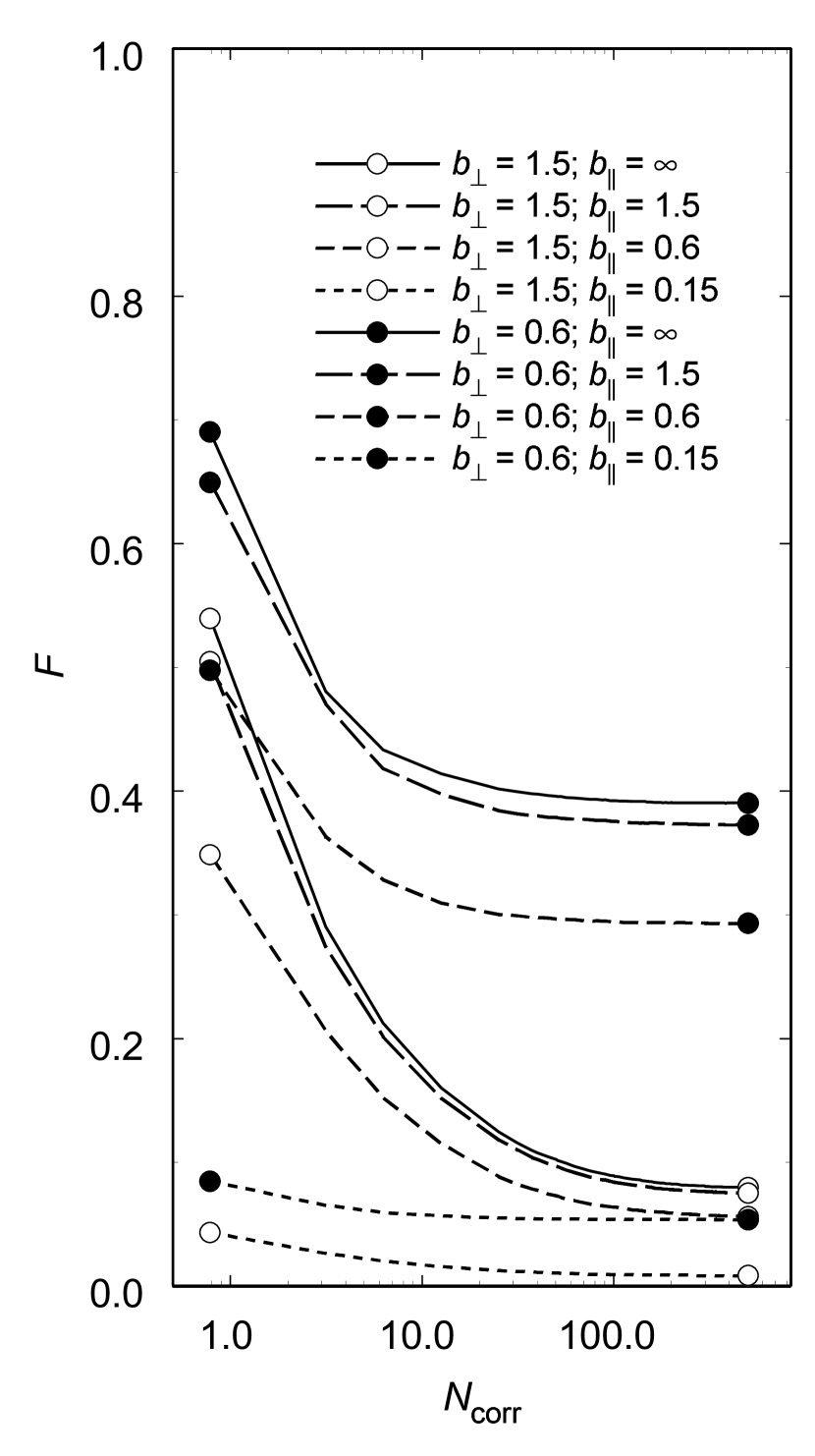
Figure 2: Polarization reduction factor $F$ due to turbulence and with a non-zero LOS magnetic field. Weak and strong field cases are indicated by open and filled circles, respectively. Solid lines ($b_{\|}=\infty$) are computed when the uniform magnetic field component along the LOS is zero.

The simplification that the uniform magnetic field is parallel to the plane of the sky is relaxed in Figure 2, and a non-zero line of sight (${\|}$-component) $B_{\mathrm{avg}}^{\|}$ is allowed. Specifically, we compute $F$ for the same two values of $b_{\bot}$ as in Figure 1 with a range of finite values for $b_{\|}$. Note that $\sigma_{\alpha}$ does not depend on $b_{\|}$ so that the anglular dispersions $\sigma_{\alpha}$ for the computations in Figure 2 are given by the right-hand panel of Figure 1 for the same $b_{\bot}$.

The solid lines with filled and open circles correspond to the two cases shown in Figure 1, where the uniform magnetic field along the line-of-sight is zero. When $B_{\mathrm{avg}}^{\|}\neq 0$, the asymptotic value depends upon $b_{\|}$ as would be expected from equation (8),

$$F=\frac{3}{2}\left(\langle\cos^{2}\theta\rangle-\frac{1}{3}\right)\cos^{2}\gamma.$$ (13)

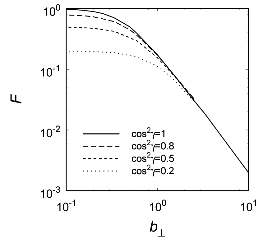
Figure 3: Asymptotic values of $F$ ($\equiv F_{\infty})$ versus $b_{\bot}$ for representative values of $\cos^{2}\gamma$.

However, as can be seen from Figure 3 where asymptotic values $F_{\infty}$ are plotted versus $b_{\bot}$ for some representative values of $\cos^{2}\gamma$, the dependence of the computed $F_{\infty}$ on $\theta$ and $\gamma$ does not, in general, separate cleanly as in equation (13). In fact, equation (8) only seems to express the dependence of $F_{\infty}$ on the line-of-sight magnetic field when $b_{\bot}\lesssim 0.5.$ For $b_{\bot}\gtrsim 1$, $F_{\infty}$ in Figure 3 becomes essentially independent of the line-of-sight magnetic field. In other words, if the turbulent magnetic field is only a factor of 1.5 greater than the component of the uniform magnetic field in the plane of the sky, $F$ does not depend on the LOS magnetic field component, whether it is weak or strong. This means that our conclusions about the polarization properties of the dust thermal emission are essentially insensitive to the LOS magnetic field component for the weak field case ($b_{\bot}=1.5$) that is considered, provided $\gamma<70^{\circ}$. The number of correlation lengths needed to reach an asymptotic value is aproximately the same for any $b_{\|}$.

3.2 Finite Beam Size

To examine the influence of the finite size of a telescope beam, we smooth the computed map for $b_{\|}=0$ to represent various angular resolutions. As might be expected, the important parameter in this case is not the ratio of a beam size to the extent of the map, but the ratio $S$ of the beam size to the correlation length $L_{\mathrm{corr}}$. This is illustrated in Figure 4, where $F$ and $\sigma_{\alpha}$ are presented for three cases in which the ratio of the beam size to $L_{\mathrm{corr}}$ is the same ($S=1.6$), though the dimensions of the computational cubes as measured in terms of correlation lengths are different. The areas of the cube surface that are viewed by the beams are adjusted appropriately. Note that $L_{\mathrm{corr}}$ is expressed in Figure 4 and elsewhere as a fraction of the length of an edge of a computational cube.

In Figure 5, $F$ and $\sigma_{\alpha}$ are presented for several representative beam sizes as measured in correlation lengths. When the beam size is much smaller than $L_{\mathrm{corr}}$, $F$ and $\sigma_{\alpha}$ are the same as for the case of the infinitesimal beam. However, if the beam size is larger than the correlation length, the requirement that there be many correlation lengths through the cloud in order for $F$ to reach $F_{\infty}$ is relaxed. The observed polarization can be close to its asymptotic value even if $N_{\mathrm{corr}}<10$.

From the point of view of obtaining inferences about the strength of the magnetic field, this means that low-resolution (or smoothed high-resolution) mapping is preferable. The procedure described by Novak et al. (1997) for the large $N_{\mathrm{corr}}$ limit can then be applied to determine the ratio of the irregular-to-average components of the magnetic field even if $N_{\mathrm{corr}}$ is relatively small or unknown. This straightforward way to infer the irregular-to-average magnetic field ratio is valid only if the average magnetic field is not inclined significantly to the plane of the sky (that is, $b_{\|}$ must be small). A large $||$-component of the magnetic field greatly complicates the interpretation. In fact, an inspection of Figures 2 and 5 shows that the curve in Figure 2 for a very strong magnetic field ($b_{\bot}=0.6$ and $b_{\|}=0.15$) looks quite similar to the dotted curve in the upper left panel of Figure 5 which corresponds to a uniform magnetic field that is weaker than the turbulent magnetic field, but is observed with a large beam.

The rms angle $\sigma_{\alpha}$ decreases with increasing beam size, and even for $b_{\bot}=1.5$ becomes smaller than $10$ degrees for clouds that are no thicker than about ten correlation lengths when $S\sim 3$ in Figure 5. This may explain why the measured dispersion of the position angle in some observations is comparable to the observational error (Ward-Thompson et al., 2000).

For a given value of $b_{\bot}$ $(b_{\|}=0)$, both $F$ and $\sigma_{\alpha}$ in Figure 5 depend on $N_{\mathrm{corr}}$ and $S$. However, we find that to a reasonable approximation these two quantities can be combined into a single quantity $G_{\mathrm{corr}}$ that describes their effect and can be understood as a generalized measure of the number of “correlation cells” that are traversed by rays received by a telescope. We define $G_{\rm corr}$ as the square of the sum of the square root of the thickness of the cloud and the area of the telescope beam expressed in correlation lengths

$$G_{\mathrm{corr}}=\left(N_{\mathrm{corr}}^{1/2}+S\right)^{2}.$$ (14)

The validity of this expression is demonstrated in the right-hand-side of Figure 5, where $F$ and $\sigma_{\alpha}$ are shown as functions of $G_{\mathrm{corr}}$. Equation (14) shows that if $N_{\mathrm{corr}}$ is comparable to $S$, changes in $S$ tend to be more important for $F$ and $\sigma_{\alpha}$ than are changes in $N_{\mathrm{corr}}$. When the number of correlation lengths along a ray is large, $G_{\mathrm{corr}}\approx N_{\mathrm{corr}}$. A rigorous analysis may give a more conceptually based relationship for $G_{\mathrm{corr}}$. However, the expression (14) serves well for the illustrative purpose in this paper.

Although $F$ and $\sigma_{\alpha}$ each depend on the thickness of the cloud and upon the beam size (as measured by $S$), the plot of $F$ as a function of $\sigma_{\alpha}$ does not depend upon these two quantities. Curves representing $F$ versus $\sigma_{\alpha}$ are shown in Figure 6 for two values of the magnetic field ratio $b_{\bot}$. We have performed computations with a number of choices for $N_{\mathrm{corr}}$ and $S$ to verify that the relationship between $F$ and $\sigma_{\alpha}$ is, in fact, independent of these quantities.

Also shown in Figure 6 are observational data for a selection of large molecular clouds and individual globules (both with and without embedded sources). The data for OMC-1, M17, W51, and W3 are taken from Dotson et al. (2000) and Schleuning et al. (2000). Data for NGC 7538 are taken from Momose et al. (2001). Data for OMC-3 are taken from Matthews et al. (2001). For each object, the average polarization $\bar{p}$ and the “true” dispersions of $p$ and $\alpha$ are computed from

$$\sigma_{p}^{2}=\mathrm{var}\,{p}-1/\sum(1/\sigma_{p,i}^{2})$$ (15)

and

$$\sigma_{\alpha}^{2}=\mathrm{var}\,{\alpha}-1/\sum(1/\sigma_{\alpha,i}^{2}).$$ (16)

where $\sigma_{p,i}$ and $\sigma_{\alpha,i}$ are the observational errors that are provided by the observers. We exclude points with $p/\sigma_{p}<3$ as unreliable, as well as points that apparently (based on the position angle histogram) belong to a component that is different from the “main” component. Data for CB 26, CB 54, and DC 253–1.6 are taken from Henning et al. (2001). As no tables are given in the latter paper, all the needed numbers are extracted from the text. Data for L1544, L43, and L183 are based on the paper by Crutcher et al. (2004) and kindly provided by its authors.

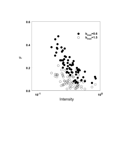
Figure 15: Polarization reduction factor $F$ as a function of intensity for variable $b_{\bot}$.

The wavelengths of the observations are indicated in the caption. It is well known that polarization is wavelength-dependent. Hence, the data points obtained at different $\lambda$ cannot, in principle, be compared directly, unless they are reduced to a single wavelength with some correction factors like those implied by Figure 15 from Hildebrand et al. (2000). However, there may be considerable spread in these factors from object to object (Vaillancourt, 2002), so we choose to make no wavelength correction of any kind. In the relevant range of $\lambda$ ($100-850\,\mu$m) these factors are near unity.

To relate the observed percentage polarization to the $F$ that is computed, it is necessary to know the polarization that is produced by the grains when the magnetic field is completely uniform. Hildebrand & Dragovan (1995) estimated that the maximum polarization produced by the mixture of perfectly aligned silicate and graphite grains ($R=F=1$) should be about 35% at $\lambda=100$ $\mu$m for their particular grain shape. We assume that the reduction from the theoretical maximum of 35% to the maximum polarization that is observed ($\sim 15\%$) occurs entirely because of imperfect grain alignment and there is no contribution due to any irregularity of the magnetic field ($R\simeq 0.4$). Thus, to compare the observational data with the computed $F$, we adopt $F_{\rm obs}=p_{\mathrm{obs}}/(R\cdot 35\%)$.

The data points in Figure 6 lie mostly in the region bounded by the two computed curves. This tends to indicate that the uniform magnetic field in these objects is comparable with the random field or does not exceed it by much. Of course, there is considerable uncertainty in relating the observations to the computations in Figure 6 because of the poor knowledge of $R$. Without information about $R$, values of $\bar{p}$ and $\sigma_{\alpha}$ can only be used to provide general guidance about the ratio of the irregular to the uniform magnetic field. With this limitation in mind, Figure 6 demonstrates the key result—that the observed average polarization properties of interstellar clouds are consistent with irregularities in the magnetic field and a uniform magnetic field that is relatively weak, as we favored in Wiebe & Watson (2001).

A non-zero component of the uniform magnetic field that is parallel to the line of sight does not affect $\sigma_{\alpha}$, but does tend to reduce $F$ and hence shifts the computed curves downward in the left hand panel of Figure 6. As long as this parallel component is similar to or less than the perpendicular component of the uniform field, its effect (see Figure 2) will be to shift the curve for $b_{\bot}=0.6$ downward by no more than about 0.1 in $F$ and to leave the curve for $b_{\bot}=1.5$ essentially unchanged. The data in Figure 6 would still be consistent with the relatively weak uniform magnetic field.

A quantity that is free from the uncertainties in $R$ is the relative polarization dispersion, $\sigma_{F}/F$. In the right hand panel of Figure 6, this quantity is plotted as a function of $\sigma_{\alpha}$. The relationship $\sigma_{\alpha}=28.6^{\circ}\sigma_{F}/F$, that would be expected for statistically independent $q$ and $u$, only holds for small $\sigma_{\alpha}$. For $\sigma_{\alpha}>10^{\circ}$, the value of $\sigma_{F}/F$ is only weakly sensitive to $b_{\bot}$. It also does not depend on the beam size, though this is not shown explicitly. On the other hand, it grows somewhat for large $b_{\|}$. Thus, a relative polarization error that is greater than unity can be indicative of a significant line-of-sight component of the magnetic field. With the few exceptions, almost all the observational points are concentrated near the computed values. Note that $\sigma_{\rm{F}}$ and $\sigma_{\alpha}$ in Figure 6 are not observational errors, but actual dispersions caused by the variations of the magnetic field.

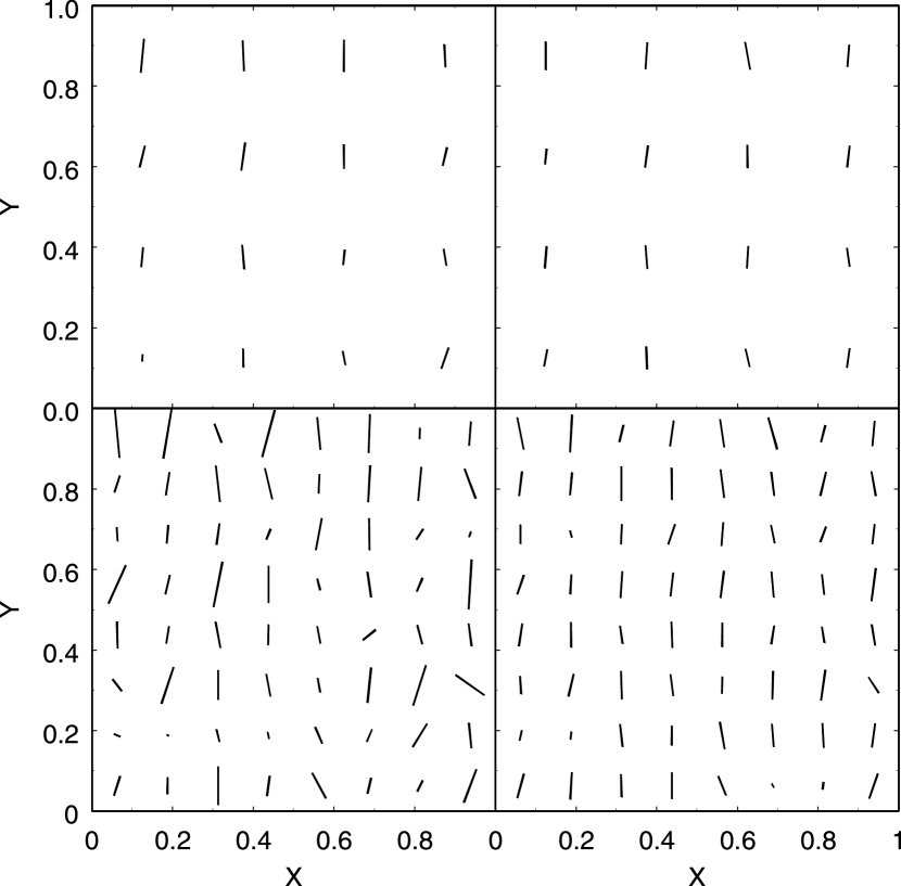
Figure 7: Computed maps of polarization vectors with the weak, uniform magnetic field for two values of $N_{\rm corr}$ (left column, $N_{\rm corr}=12$; right column, $N_{\rm corr}=36$) and for two values of $S$ (top row, $S=3.2$; bottom row, $S=1.6$). Coordinates are given as a fraction of the distance along the face of the computational cubes. The longest vector corresponds to $F=0.18$. The uniform field is in the $x$ direction. Position angle dispersions are $8^{\circ}$ (left) and $7^{\circ}$ (right) for the top row, and $21^{\circ}$ (left) and $11^{\circ}$ (right) for the bottom row.

In Figure 7 we show the maps of polarization vectors that have been used to compute the average values presented in the foregoing. Maps are shown for two values of $N_{\rm corr}$—the number of correlation lengths traversed along each ray. The maps are smoothed with beam sizes of $S=1.6$ and 3.2. They correspond to dotted and short-dashed lines on the leftmost panels of Figure 5. While the mean polarization is close to its asymptotic value on these maps, there are regions where $F$ exceeds this value almost by a factor of 2. Even though the uniform magnetic field is weak, the polarization shows a regular pattern at $N_{\rm corr}\sim 30$, when the beam size is comparable to the correlation length, and at $N_{\rm corr}\sim 10$, when the beam size is greater than $L_{\rm corr}$.

We conclude that the irregularities in the magnetic field used in Wiebe & Watson (2001) to understand the polarized absorption of starlight are not in conflict with the observed polarization properties of the thermal radiation that is emitted by dust grains, provided that the correlation lengths in the regions that have been investigated are somewhat smaller than the sizes of the telescope beams. It is more difficult to understand how a polarization hole can appear in such an environment. Along with the regions of high polarization, there are some spots in Figure 7 where $F$ is much smaller than the mean value. Inspection of the underlying map for the infinitesimal beam size shows that this is due to the higher than average magnetic field tangling in the particular regions. If for some reason disturbances in the magnetic fields in actual gas clouds are associated with the density enhancements, such regions will be observed as polarization holes. This issue is further addressed in the next Section. However, in general, it is unlikely that a polarization holes will be due to this cause alone. From Figure 1, the decrease in the percentage polarization can be caused either by an increase in the number of correlation lengths or by a weakening of the mean magnetic field (or both) in a dense region where the hole is observed. However, in the weak uniform field case and at $N_{\rm corr}>10$, which is preferable for our proposed interpretation of the polarization of starlight, $F$ already is about as small as it can be (especially, when the finite beam size is taken into account), leaving little space for further decrease.

On the other hand, the magnetic field structure may cause polarization holes if for some reason the uniform field is stronger on a periphery of a dense object and weakens closer to its center. If the decrease of polarization with growing intensity is caused by shorter correlation lengths, one would expect that $\sigma_{\alpha}$ is smaller in dense cores than in the surrounding medium. Interesingly, this is what actually is observed in some cores of Barnard 1 dark cloud (Matthews & Wilson, 2002).

4 Density Effects

In the previous section we concluded that the unresolved magnetic field structure cannot be a common reason for the polarization hole effect. In this Section we investigate whether the polarization hole effect can be due to effects that are related to the variations in density.

We generate the spatial distribution of dust by the same procedure that we used to create the magnetic field. A single component of the vector field is created in the Fourier space with the same $k_{\min}$ as is used to generate the magnetic field. This distribution of Fourier waves is inverted to find the distribution in coordinate space. The resultant Gaussian quantity is interpreted as the logarithm of the density. The density created in this way has a log-normal probability distribution function (PDF) that possesses the desired spatial variations as characterized by the correlation length. The volume weighted distribution of the quantity $y\equiv\log(n_{\mathrm{d}}/\bar{n}_{\mathrm{d}})$, where $n_{\mathrm{d}}$ and $\bar{n}_{\mathrm{d}}$ are the actual and spatially averaged densities of dust grains, is

$$f(y)={\frac{1}{\sqrt{2\pi\sigma^{2}}}}\exp\left[-{\frac{(y+|\mu|)^{2}}{2\sigma^{2}}}\right].$$ (17)

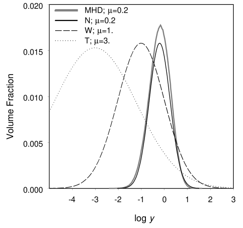
Figure 8: Density distributions that are utilized in the computations. The distribution ‘N’ (‘narrow’) is chosen to be as close as possible to the results of Stone et al. (1998), which are indicated by the thick gray line. Distribution ‘W’ (‘wide’) is intended to represent results of other numerical simulations that lead to a wider density PDF. The distribution used to study thermalization effects is labelled with ‘T’.

The log-normal PDF seems to be relevant in the isothermal case and is reproduced in many MHD simulations (Nordlund & Padoan 1999; Vázquez-Semadeni et al. 2000; Ostriker et al. 2001). In Figure 8 we compare the PDFs for our simulated densities with that of the MHD simulation by Stone et al. (1998). The corresponding $|\mu|$ values are given in the legend. To assess the importance of the spatial structure of the density field, distributions with different numbers of correlation lengths ($N_{\mathrm{corr}}=5$ and 12) through the computational cube are considered. The polarization reduction factor $F$ in this Section thus includes the reduction of polarization due not only to tangling of the magnetic field, but also due to the various additional factors that are studied here. The correlation length is assumed to be independent of density.

4.1 A Density Cutoff for Polarization

In this subsection we examine the consequences of the assumption that dust grains lose their ability to polarize light as the density increases. This might be due to poor alignment caused by more frequent collisions with the gas molecules or to the growth of icy mantles that make the grains more spherical. A similar suggestion was recently studied by Padoan et al. (2001). They showed that it is possible to reproduce the observed anticorrelation between $P$ and $I$ under the assumption that grains are not aligned at depths beyond a certain value of extinction $A_{\mathrm{V}}$ measured from the edges of the clouds. This assumption implies that radiative torques are the primary cause for grain alignment.

Here, we assume that grains are no longer aligned when the density exceeds a certain critical density $n_{\lim}$. That is, in equations (5) and (6) we assume that

$$n^{\mathrm{a}}_{\mathrm{d}}=\left\{\begin{array}[]{ll}n_{\mathrm{d}}&n_{\mathrm{d}}\leq n_{\lim}\\ 0&n_{\mathrm{d}}>n_{\lim}\end{array}\right..$$ (18)

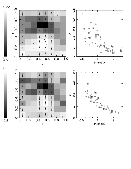
Figure 9: Map of polarization vectors and $F$ vs $I$ diagram for the ‘N’ distribution and the strong uniform magnetic field. Upper panel, $N_{\mathrm{corr}}=5$, lower panel, $N_{\mathrm{corr}}=12$. The longest vector corresponds to the highest $F$. The map is obtained by averaging over $16\times 16$ emerging rays. The grayscale on left panel and the scale of the horizontal axis on right panel is the intensity of dust emission in arbitrary units. The uniform magnetic field is in the $x$ direction.

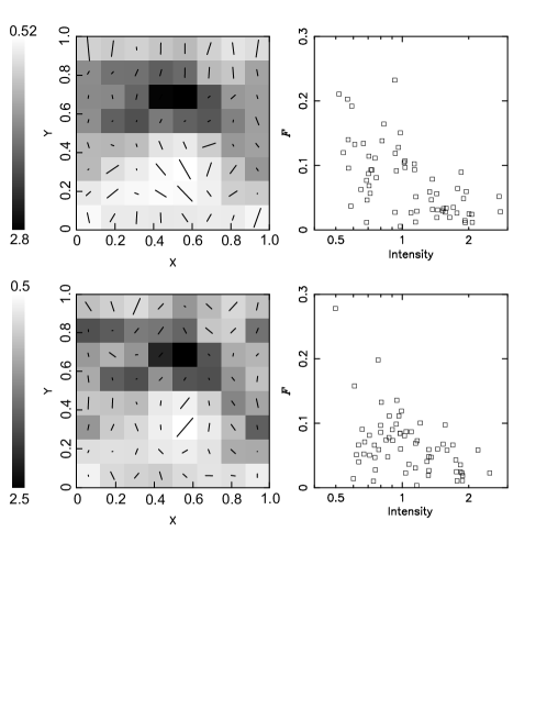
Figure 10: Same as in Figure 9, but for the weak uniform magnetic field.

First we consider the density distribution that corresponds most closely to the distribution from the MHD calculations (labeled ‘N’ in Figure 8). Intensity maps overlaid with the polarization vectors and the $F$ vs $I$ scatter diagrams for the ‘N’ distribution are shown in Figures 9 and 10. The density cutoff is set as 1.7 times the median density. The upper panels of the Figures correspond to calculations for which the number of correlation lengths along the side of the map $N_{\mathrm{corr}}\approx 5$. In the calculations for the lower panels $N_{\mathrm{corr}}\approx 12$. The uniform magnetic field is strong ($b_{\bot}=0.6$) in Figure 9, and is weak ($b_{\bot}=1.5$) in Figure 10. It is noteworthy that the densities at almost 30% of the grid points exceed the specified critical density and thus do not contribute to $Q$ and $U$. If we assume that the side of the computational cube is 1 pc (so that the diameter of the central concentration in upper panels is about a few tenths of a parsec and $L_{\rm corr}\sim 0.1$ pc), the optical depth $\tau\approx 10^{-3}$ for the ‘N’ distribution corresponds to a median gas density of approximately $10^{4}$ cm^-3 at $\lambda=1.3$ mm (where a dust opacity $\kappa_{1.3\,\mathrm{mm}}=1$ cm² g^-1 is assumed; Ossenkopf & Henning 1994). To produce the observed decrease in polarization, dust grains should be unaligned in all clumps that are at least moderately dense for these calculation with the ‘N’ distribution. This seems to contradict the fact that highly polarized dust emission is sometimes observed from regions that are even more dense.

Even under these rather extreme conditions, the scatter diagram for $F$ vs $I$ for the weak field case is far from the tight appearance actually seen in many observations—at least, at long wavelengths. In the strong field case, the tightness of the correlation depends upon the specific realization at this $n_{\lim}$; i. e. in some statistical realizations of the density the scatter can be more significant. If $n_{\lim}$ is increased by only by a factor of a few, the correlation between the percentage polarization and the intensity completely disappears. Lower values of $n_{\lim}$ tend to produce tight correlations in any realization, though the percentage polarization is quite low. If we set $n_{\lim}$ equal to the median density, the maximum $F$ (at the lowest intensity) is only about 0.1 even for the strong field. The observed slope—a decrease by a factor of about 3 in percentage polarization as the intensity grows by an order of magnitude—is only reproduced by the strong field and low $N_{\mathrm{corr}}$.

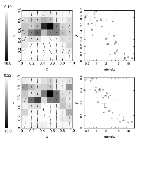
Figure 11: Map of polarization vectors and $F$ vs $I$ diagram for the ‘W’ distribution and the strong uniform magnetic field. Upper panel, $N_{\mathrm{corr}}=5$, lower panel, $N_{\mathrm{corr}}=12$. Intensity is in arbitrary units. The longest vector corresponds to the highest $F$. The map is obtained by averaging over $16\times 16$ emerging rays. The grayscale on left panel and the scale of the horizontal axis on right panel is the intensity of dust emission in arbitrary units. The uniform magnetic field is in the $x$ direction.

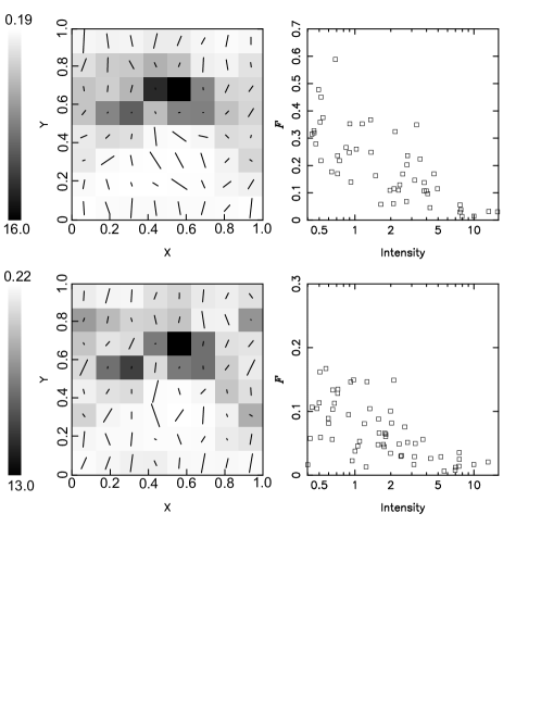
Figure 12: Same as in Figure 11, but for the weak uniform magnetic field.

In other models of HD and MHD turbulence the density distribution can be wider, with the range in densities reaching six orders of magnitude (Padoan et al. 1998; Klessen, Heitsch, & Mac Low 2000). Hence, we introduce a wider PDF labeled ‘W’ in Figure 8. With the same choice of fiducial parameters, the median density is $\sim 4\times 10^{3}$ cm^-3. The high density tail of the distribution extends to $\sim 10^{8}$ cm^-3, albeit the number of high density cells is small. Thus, only a tiny fraction of the volume contributes to the dust emission. In such a wide distribution, the tight correlation between $F$ and $I$ can be reproduced with a much higher value of $n_{\lim}$. Maps and diagrams for the wide density PDF and $n_{\lim}\approx 50n_{\mathrm{med}}$ are shown in Figures 11 and 12. Only 4% of the grid points do not contribute to the polarized emission by this criterion. This seems sufficient to obtain (at least in most realizations) a rather tight $F$ and $I$ correlation in the strong field case. The weak magnetic field tends to produce more scatter, though $F$ at low intensity is quite high in all four cases that we present— reaching value of 0.7 for the strong uniform field and $N_{\mathrm{corr}}=5$. In all cases except the last, $F$ decreases significantly with intensity, in agreement with observations. To summarize, increasing $n_{\lim}$ leads to more scatter; decreasing $n_{\lim}$ produces tighter correlations but smaller $F$.

4.2 Thermalization Effects

It is widely assumed that the emission by dust from the star forming regions is optically thin. Nevertheless, unresolved optically thick clumps are sometimes mentioned (e.g. Gull et al. 1978; Schleuning 1998; Schleuning et al. 2000) along with other possible causes for the decrease in the percentage polarization in the brightest regions of dense clouds. Clearly, this mechanism is most likely to be effective in star forming regions where high opacities and submillimeter luminosities are expected for Class 0 objects (André, Ward-Thompson, & Barsony 2000). Optical depths of order of 1 are implied both at the far-infrared (Larsson et al. 2000; Mookerjea et al. 2000) and in the submillimeter range (Sandell 2000; Sandell & Knee 2001) in the dense parts (cores) of at least some star forming regions.

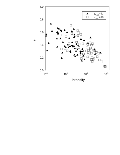
Figure 13: Polarization reduction due to effects of thermalization.

We will examine, to a limited degree and only in Figure 13, the consequences of the thermalization that occurs when the optical depth approaches and exceeds one. For this, the previous expressions must be generalized somewhat. The optical depth becomes

$$\tau=\tau_{0}\int n_{\mathrm{d}}ds$$ (19)

where $\tau_{0}$ is the normalization factor, and the expressions for relative Stokes parameters are

$$\begin{array}[]{l}i=1-e^{-\tau}\\[2.84544pt] q=\tau_{0}e^{-\tau}\int n_{\mathrm{d}}\cos^{2}\gamma^{\prime}\cos 2\phi ds\\[2.84544pt] u=\tau_{0}e^{-\tau}\int n_{\mathrm{d}}\cos^{2}\gamma^{\prime}\sin 2\phi ds.\end{array}$$ (20)

These expressions allow the emission by dust to be optically thick, but still assume that the fractional polarization is small.

To investigate the effect of large optical depth, we utilize an even wider density distribution (labeled ‘T’ in Figure 8) to calculate $F$ for three different values of $\tau_{0}$ which are chosen so that the maximum optical depth along any ray is $\tau_{\max}=1$, or 10, or 100. There is no density cutoff for grain alignment in this case. Results for the second and the third cases are shown in Figure 13. At $\tau_{\max}=1$, no trend of decreasing polarization with increasing intensity is evident. It starts to appear at $\tau_{\max}=10$, where the properties of the density field are still realistic. With the adopted fiducial parameters, at $\lambda=1.3$ mm the ‘T’ density PDF results in a few rarified cells ($n\sim 1$ cm^-3) and a few very dense cells (with the peak gas density $n\approx 2\times 10^{10}$ cm^-3). The median density for the entire cube is $10^{3}$ cm^-3, and median optical depth is $\sim 5\times 10^{-3}$ (for the far-infrared waveband, all densities are an order of magnitude lower due to the higher opacity).

However, a slope that is similar to what is observed is only achieved when $\tau_{\max}=100$ and with a median optical depth $\sim 10^{-2}$, which probably is too high for the submillimeter waveband. Thus, we conclude that thermalization probably is not important for explaining the polarization holes observed at longer wavelength, though it may contribute to this effect in the far-infrared.

4.3 Effects of Correlations between the Density and the Magnetic Field

The procedure that we use to generate the matter densities does not lead to distributions for the matter and magnetic fields that are consistent with one another. Specifically, in the previous subsections we used the same ratio of the turbulent to the uniform magnetic field $b_{\bot}$ for the entire cube, despite the variations in density. In reality, we may expect that the spatial distributions of density and of the magnetic field are not independent. In Figure 14 we plot the standard deviations of the 3D magnetic field along each ray versus the column density in arbitrary units for an MHD simulation (weak uniform field case) by Stone et al. (1998). Though the lower part of the plot is more densely populated, a trend is evident. For clarity, only each 100th point is shown for column densities less than 400. A similar trend is observed in the cube computed with the strong uniform field. Thus, in the available MHD simulations, the magnetic field does exhibit a stronger variation along the rays with higher optical depth— though the range in density is not wide.

In our model, the ability to reproduce this correlation between the matter density and the magnetic field is quite limited. To evalute its importance semi-quantitatively, we calculate a model in which $b_{\bot}$ is proportional to the local density and is normalized to be equal to a specific value at the median density, designated as $b_{\mathrm{med}}$. The ‘N’ density PDF is utilized at $N_{\mathrm{corr}}=12$ (these parameters are chosen to reproduce the results of the MHD simulations as closely as possible). There is no density cutoff for the alignment of the grains. In Figure 15 we show $F$ and $I$ for the calculations with $b_{\mathrm{med}}=1.6$ and $b_{\mathrm{med}}=0.5$. For the two cases that are presented, the magnetic field ratios in most grid cells correspond to those of our weak and strong fields, respectively. At the low density end of the distribution, the magnetic field is strictly uniform; at the high density tail, there is essentially no uniform field.

The decrease in $F$ with increasing intensity is present in both cases, though only the strong field ($b_{\rm med}=0.6$) reproduces the observed slope. If we use the same scaling of $b_{\bot}$ with density and the ‘W’ density PDF, the trend is absent both in the weak and the strong field cases. It only reappears at $b_{\mathrm{med}}<0.2$. However, this scaling probably is not appropriate for the ‘W’ distribution, which is intended to describe the more advanced evolutionary stages of the star forming regions.

5 Discussion

The polarization of starlight due to absorption by dust and the polarization of the thermal emission from dust provide two ways to study the structure of the magnetic field in star forming regions. However, observations indicate that tracing the direction of the magnetic field with polarized starlight can be seriously hindered by some factor or factors that prevent the grains in the dark interiors of clouds from influencing the observed polarization. In Wiebe & Watson (2001) we argued that a relatively strong turbulent magnetic field within dark clouds may sufficiently randomize the orientations of the dust that their contributions to the polarization of starlight effectively cancel. If a ray of starlight is initially polarized by passing through the general interstellar medium with $b_{\bot}\sim 0.5$, and then traverses about 10 correlation lengths within a cloud where $b_{\bot}$ is about 3 times greater, its polarization is almost unchanged in magnitude and in direction as a result of passing through the cloud.

In this paper we show that the occurence of such irregular magnetic fields in dark clouds is not in conflict with the relatively ordered polarization vectors of the dust emission observed both in quiescent dense cores and in the regions of ongoing star formation. The maps of polarization vectors that are computed using a medium with relatively strong turbulent magnetic fields and with large $N_{\rm corr}$ show the regular patterns typically seen in the infrared and submillimeter observations. The average percentage polarization within these maps is $2-4\%$ (assuming $R\approx 0.4$), and is close to what is observed. Heitsch et al. (2001) reached similar conclusions about the polarized emission for certain specific turbulent MHD models for the medium. Chance misalignment of polarization vectors in adjacent points can cause a decrease in the percentage polarization—reminiscent of polarization hole—if this region is observed with low angular resolution.

In the context of the polarization hole effect, Figure 1 suggests that the decrease in the percentage polarization can be a result of the larger number of correlation lengths that a ray traverses in passing through a dense core versus the number it traverses in the surrounding medium. For this, $N_{\mathrm{corr}}$ in the surrounding medium must be small because the polarization reduction factor $F$ reaches its asymptotic value quite fast. For the moderately strong uniform field ($b_{\bot}=0.6$), $F$ is essentially $F_{\infty}$ when $N_{\mathrm{corr}}$ is approximately a few. In the case of the weak uniform field ($b_{\bot}=1.5$) that we favored in Wiebe & Watson (2001), a factor of a few decrease in $F$ is achieved between $N_{\mathrm{corr}}\sim 1$ and 30. Over the same range of $N_{\mathrm{corr}}$, $\sigma_{\alpha}$ decreases from 40^∘ to about 20^∘.

These values for $N_{\mathrm{corr}}$ and $\sigma_{\alpha}$ are larger than the values that are indicated from the observations. The need to have $N_{\mathrm{corr}}$ near 30 is relaxed if we take into account a finite beam size and allow the correlation length $L_{\mathrm{corr}}$ to be smaller in the core than on the periphery. Let us assume that on the periphery of a dense core, a ray traverses $N_{\mathrm{corr}}\sim 1-3$ and that the beam size is smaller than $L_{\mathrm{corr}}$. In this case $F$ is about $0.4-0.5$ (the solid or long-dashed curve on the top left panel of Figure 5). If toward the center of the dense core $L_{\mathrm{corr}}$ becomes smaller than the beam size, then $F\sim 0.1$ toward the center (the dotted curve on the top left panel of Figure 5). With this beam size and with $N_{\mathrm{corr}}\sim 10$, $\sigma_{\alpha}$ becomes less than 10^∘. If the same region is observed with a smaller beam (e.g., with an interferometer), then the dispersion in position angles would increase (because $G_{\mathrm{corr}}$ becomes smaller).

The apparent discrepancy in this scenario of a large dispersion in position angles at the periphery of the core ($\sim 40^{\circ}$) can be partially circumvented by assuming that the strength of the uniform magnetic field is higher in the vicinity of the core than in the core itself. When $b_{\bot}=0.6$ in the periphery region, $\sigma_{\alpha}$ can be as small as 20^∘ (solid curve on the lower right panel of Figure 5 at $N_{\mathrm{corr}}=3$). It is even smaller at lower $b_{\bot}$.

The requirement that a ray traverse only a few correlation lengths in a region surrounding the dense core where the polarization hole is observed may also seem to conflict with our conclusion in Wiebe & Watson (2001) that a typical dark cloud spans no fewer than 10 correlation lengths. It must be noted that in the B1 cloud, where polarimetry observations of both starlight and thermal dust emission are available, they indicate different directions for the magnetic field (Matthews & Wilson, 2002). It is quite possible that the polarized light of background stars and the polarized dust emission, even when they are observed close to one another, trace different objects or parts of the same object that differ in physical conditions and/or scale. The two types of observations may thus not be directly related to one another. In addition, observations of starlight polarization are mostly used to study quiescent dark clouds, while many (though not all) objects in which the polarization of the dust emission is observed already contain Class 0 protostars with outflows.

Our calculations demonstrate quantitatively how the magnitude of the correlation length (or at least how the correlation length compares with the size of a cloud and the size of the telescope beam) is the key factor for the influence of turbulence on the observations of the linear polarization. Unfortunately, any suggestions based on our calculations that we can offer for extracting the correlation length from observational data are hampered by the lack of information about $R$ and about the source geometry. With these limitations in mind, some inferences about $N_{\rm corr}$ can be made based on Figures 5 and 6 and an application of equation  (14). Assuming that the number of correlation lengths is the same along the line of sight and perpendicular to it, we may replace $S$ in equation (14) with $N_{\rm corr}/D$, where $D$ is the number of beams across an object. Equation (14) then can be solved for $N_{\rm corr}$ in terms of $G_{\rm corr}$.

Let us consider two examples. The location of the L1544 core in left panel of Figure 6 implies that the uniform magnetic field is strong in this object. The polarization position angle dispersion $\sigma_{\alpha}$ then corresponds to $G_{\rm corr}\sim 10$ (see right panel of Figure 5). For these observations, $D\sim 8$ and we obtain $N_{\rm corr}\sim 5$. Assuming the generally accepted distance of 140 pc and an angular size of about $110^{\prime\prime}$ (Ward-Thompson et al., 2000) gives $L_{\rm corr}\sim 0.02$ pc for this object. The L43 core, on the other hand, in left panel of Figure 6 is located close to the curve corresponding to the weak uniform field. The small anglular dispersion implies $G_{\rm corr}\sim 50$ according to Figure 5 (right panel), which for the same $D$ gives $N_{\rm corr}\approx 20$. At a distance of 170 pc and an angular size of $\sim 100^{\prime\prime}$ (Ward-Thompson et al., 2000), $L_{\rm corr}\sim 0.004$ pc. Determinations of the correlation lengths by independent methods would be valuable. Unfortunately, the tendency for velocity shifts in clouds to be caused by large-scale velocity gradients as well as by turbulence, for the presence of inhomogeneities in cloud properties, etc. obscure the detailed effects of turbulence .

This work was supported in part by NSF Grant AST 9988104. DW acknowledges support from the President of the RF grant MK-348.2003.02.

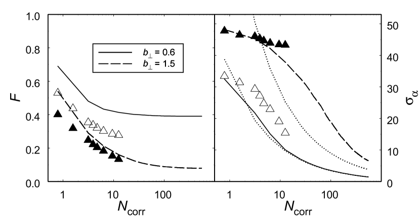
Figure 1: Polarization reduction factor $F$ due to turbulence and the dispersion $\sigma_{\alpha}$ in the position angle vs the number of correlation lengths $N_{\mathrm{corr}}$ through a cloud. Results from the actual MHD computations are denoted by filled ($b_{\bot}=1.5$) and open ($b_{\bot}=0.6$) triangles. The dispersion of position angles obtained with the expression of Myers & Goodman (1991) is indicated by the dotted lines.

Figure 4: Polarization reduction factor $F$ due to turbulence and the dispersion $\sigma_{\alpha}$ in the position angles vs the number of correlation lengths $N_{\mathrm{corr}}$ through the cloud for various values of the correlation length and $b_{\perp}=1.5$. The ratio of the beam size to $L_{\mathrm{corr}}$ is the same for all three sets of curves.

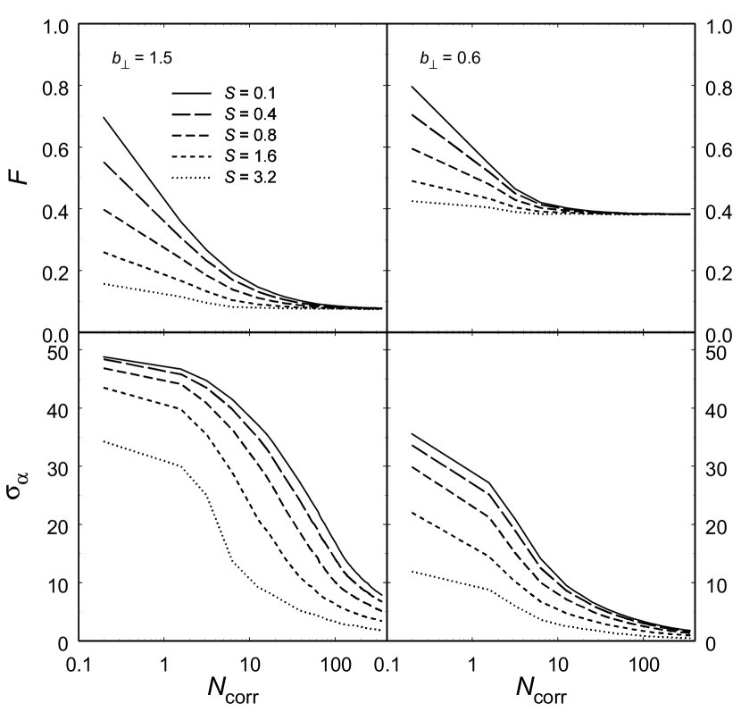
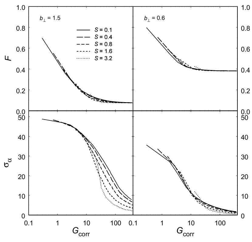
Figure 5: Left panel— $F$ and $\sigma_{\alpha}$ vs the number of correlation lengths $N_{\mathrm{corr}}$ through a cloud for different magnetic field ratios and beam sizes. Right panel—Same quantities as in left panel, but shown as functions of a generalized number of correlation lengths $G_{\mathrm{corr}}$.

Figure 6: Computed polarization reduction factor $F$ due to turbulence (left panel) and the relative polarization error $\sigma_{F}/F$ (right panel) as a function of $\sigma_{\alpha}$. Observational data also are shown for comparison. The name of the object is centered on the corresponding data point. The number 100 or 350 next to the name of the object indicates the wavelength in $\mu$m. If no number is specified, the measurement is at 850 $\mu$m. Some cloud labels have been shifted slightly for clarity

Figure 14: The rms magnetic field versus column density in the MHD simulations by Stone et al. (1998), in arbitrary units

References

- Akeson et al. (1996) Akeson, R. L., Carlstrom, J. E., Phillips, J. A., Woody, D. P. 1996, ApJ, 456, L45
- André, Ward-Thompson, & Barsony (2000) André, P., Ward-Thompson, D., & Barsony, M. 2000, in Protostars and Planets IV, ed. V. Mannings, A. P. Boss, S. S. Russell (Tucson: Univ. of Arizona Press), 59
- Arce et al. (1998) Arce, H. G., Goodman, A. A., Bastien, P., Manset, N., & Sumner, M. 1998, ApJ, 499, L93
- Crutcher et al. (2004) Crutcher, R. M., Nutter, D. J., Ward-Thompson, D., Kirk, J. M. 2004, ApJ, 600, 279
- Dickens et al. (2000) Dickens, J. E., Irvine, W. M., Snell, R. L., Bergin, E. A., Schloerb, F. P., Pratap, P., & Miralles, M. P. 2000, ApJ, 542, 870
- Dotson et al. (2000) Dotson, J. L., Davidson, J., Dowell, C. D., Schleuning, D. A., & Hildebrand, R. H. 2000, ApJS, 128, 335
- Draine & Weingartner (1996) Draine, B. T., & Weingartner, J. C. 1996, ApJ, 470, 551
- Dubinski, Narayan, & Phillips (1995) Dubinski, J., Narayan, R., & Phillips, T. G. 1995, ApJ, 448, 226
- Elmegreen & Scalo (2004) Elmegreen, B. G., & Scalo, J. 2004, ARA&A, in press [astro-ph 0404451]
- Gull et al. (1978) Gull, G. E., Houck, J. R., McCarthy, J. F., Forrest, W. J., & Harwit, M. 1978, AJ, 83, 1440
- Heitsch et al. (2001) Heitsch, F., Zweibel, E. G., MacLow, M. M., Li, P., & Norman, M. L. 2001, ApJ, 561, 800
- Henning et al. (2001) Henning, Th., Wolf, S., Launhardt, R., Waters, R. 2001, ApJ, 561, 871
- Hildebrand & Dragovan (1995) Hildebrand, R. H., & Dragovan, M. 1995, ApJ, 450, 663
- Hildebrand et al. (2000) Hildebrand, R. H., Davidson, J. A., Dotson, J. L., Dowell, C. D., Novak, G., & Vaillancourt, J. E. 2000, PASP, 112, 1215
- Hiltner (1956) Hiltner, W. A. 1956, ApJS, 2, 389
- Jones (2003) Jones, T. J. 2003, AJ, 125, 3208
- Klessen et al. (2000) Klessen, R., Heitsch, F., & Mac Low, M.-M. 2000, ApJ, 535, 887
- Larsson et al. (2000) Larsson, B., et al. 2000, A&A, 363, 253
- Lee & Draine (1985) Lee, H. M., Draine, B. T. 1985, ApJ, 290, 211
- Mathis (1986) Mathis, J. S. 1986, ApJ, 308, 281
- Matthews et al. (2001) Matthews, B. C., Wilson, C. D., & Fiege, J. D. 2001, ApJ, 562, 400
- Matthews & Wilson (2002) Matthews, B. C., & Wilson, C. D. 2002, ApJ, 574, 822
- Momose et al. (2001) Momose, M., Tamura, M., Kameya, O., Greaves, J. S., Chrysostomou, A., Hough, J. H., & Morino, J.-I. 2001, ApJ, 555, 855
- Mookerjea et al. (2000) Mookerjea, B., Ghosh, S. K., Rengarajan, T. N., Tandon, S. N., & Verma, R. P. 2000, AJ, 120, 1954
- Myers & Goodman (1991) Myers, P. C., & Goodman, A. A. 1991, ApJ, 373, 509
- Novak et al. (1997) Novak, G., Dotson, J. L., Dowell, C. D., Goldsmith, P. F., Hildebrand, R. H., Platt, S. R., & Schleuning, D. A. 1997, ApJ, 487, 320
- Nordlund & Padoan (1999) Nordlund, Å., & Padoan, P. 1999, in Interstellar Turbulence, ed. J. Franco, A. Carraminana (Cambridge University Press), 218
- Ossenkopf & Henning (1994) Ossenkopf, V., & Henning, Th. 1994, A&A, 291, 943
- Ostriker et al. (2001) Ostriker, E. C., Stone, J. M., Gammie, Ch. F. 2001, ApJ, 546, 980
- Padoan et al. (1998) Padoan, P., Juvela, M., Bally, J., & Nordlund, Å. 1998, ApJ, 504, 300
- Padoan et al. (2001) Padoan, P., Goodman, A., Draine, B. T., Juvela, M., Nordlund, Å., & Rögnvaldsson, Ö. E. 2001, ApJ, 559, 1005
- Rao et al. (1998) Rao, R., Crutcher, R. M., Plambeck, R. L., & Wright, M. C. H. 1998, ApJ, 502, L75
- Sandell (2000) Sandell, G. 2000, A&A, 358, 242
- Sandell & Knee (2001) Sandell, G., & Knee, L. B. G. 2001, ApJ, 546, L49
- Schleuning (1998) Schleuning, D. A. 1998, ApJ, 493, 811
- Schleuning et al. (2000) Schleuning, D. A., Vaillancourt, J. E., Hildebrand, R. H., Dowell, C. D., Novak, G., Dotson, J. L., Davidson, J. A. 2000, ApJ, 535, 913
- Stone, Ostriker, & Gammie (1998) Stone, J. M., Ostriker, E. C., & Gammie, C. F. 1998, ApJ, 508, L99
- Tafalla et al. (2002) Tafalla, M., Myers, P. C., Caselli, P., Walmsley, C. M., & Comito, C. 2002, ApJ, 569, 815
- Tafalla et al. (2004) Tafalla, M., Myers, P. C., Caselli, P., & Walmsley, C. M. 2004, A&A, 416, 191
- Vaillancourt (2002) Vaillancourt, J. E. 2002, ApJS, 142, 53
- Vallée et al. (2000) Vallée, J. P., Bastien, P., & Greaves, J. S. 2000, ApJ, 542, 352
- Vázquez-Semadeni et al. (2000) Vázquez-Semadeni, E., Ostriker, E. C., Passot, T., Gammie, C. F., & Stone, J. M. 2000, in Protostars and Planets IV, ed. V. Mannings, A. P. Boss, S. S. Russell (Tucson: Univ. of Arizona Press), 3
- Wallin et al. (1998) Wallin, B. K., Watson, W. D., & Wyld, H. W. 1998, ApJ, 495, 774
- Wallin et al. (1999) Wallin, B. K., Watson, W. D., & Wyld, H. W. 1999, ApJ, 517, 682
- Wardle & Königl (1990) Wardle, M., & Königl, A. 1990, ApJ, 362, 120
- Ward-Thompson et al. (2000) Ward-Thompson, D., Kirk, J. M., Crutcher, R. M., Greaves, J. S., Holland, W. S., & André, P. 2000, ApJ, 362, 120
- Watson et al. (2001) Watson, W. D., Wiebe, D. S., & Crutcher, R. M. 2001, ApJ, 549, 377
- Wiebe & Watson (2001) Wiebe, D. S., & Watson, W. D. 2001, ApJ, 549, L115
- Young et al. (2004) Young, C. H., Jørgensen, J. K., Shirley, Y. L., Kauffmann, J. et al. 2004, ApJS Spitzer Special Edition, in press (astro-ph/0406371)