Hamiltonian Cosmological Dynamics of General Relativity

Abstract

The Hamiltonian approach to General Relativity is developed similarly to the Wheeler-DeWitt Hamiltonian cosmology, where the cosmological scale factor is treated as a time-like dynamic variable and its canonical momentum is considered as an evolution generator in the field space of events with the postulate about a physical vacuum as a state with the minimal eigenvalue of this generator.

The cosmological scale factor is extracted from the Hamiltonian General Relativity without double counting of the spatial metric determinant in contrast to the standard cosmological perturbation theory. The Friedmann-like equations in the exact theory are derived. A new version of cosmological perturbation theory keeps the form of the Newton interactions in an early Universe. We show how the considered Hamiltonian approach to GR can solve the topical problems of modern cosmology and quantum theory of gravitation.

Introduction

The status of the cosmological scale factor in the modern theory is ambiguous. The standard Hamiltonian approach to General Relativity (GR) dir ; ADM ; berg ; shw ; fadpop ignores the scale factor by the choice of the corresponding class of functions where the gauge of minimal surface dir with the unit scale factor is possible. The Wheeler - DeWitt Hamiltonian cosmology M ; WDW ; Ryan1 ; Ryan2 considers the scale factor as an independent dynamic variable. In the standard cosmological perturbation theory lif ; bard ; kodam the scale factor is treated rather as the external homogeneous field than an independent dynamic variable. From this point of view all these three branches of GR appear as three different theories.

The questions arise: What is the version of the Hamiltonian GR defined on the class of functions that includes the cosmological scale factor? What is the version of the cosmological perturbation theory, where the scale factor plays the role of an independent dynamic variable?

In the present paper, to answer these questions, we use a deep analogue between GR and Special Relativity (SR) WDW with the field space of events as the generalization of the Minkowski space of SR and the cosmological scale factor playing the role of a time-like variable in this field space.

This time-like variable and the corresponding Hamiltonian dynamics can be revealed in a specific frame of reference defined in dir ; ADM ; berg ; shw ; fadpop . Fixation of this specific frame is associated with a set of instruments for measuring fields and keeps the number of variables in contrast to fixation of gauge constraints decreasing the number of dynamic variables.

To separate the gauge transformations from the frame ones, it is natural to use the representation of the geometric interval in terms of the Cartan forms introduced in GR by Fock fock29 . The Cartan forms are gauge invariant and relativistic covariant og .

The content of the paper is the following.

In Section I, the Dirac Hamiltonian approach to GR is considered in terms of the Cartan forms in order to separate the frame transformations from the gauge ones.

In Section II, arguments are listed in favor of the solution of the topical problems of the Hamiltonian approach to GR by the choice of an evolution parameter in the field space of events as the cosmological scale factor.

In Section III, the Hamiltonian approach to GR with the cosmological dynamics is developed as a new version of cosmological perturbation theory.

I Dirac Hamiltonian approach to General Relativity

I.1 The action, metric, and symmetry

In order to state problems, we consider the Dirac approach dir to the Einstein-Hilbert action

$$S_{GR}[\varphi_{0}|e]=-\int d^{4}x\sqrt{-g}\frac{\varphi^{2}_{0}}{6}R(g),$$ (1)

where

$$\varphi^{2}_{0}=\frac{3}{8\pi}M^{2}_{\rm Planck},~{}~{}~{}\hbar=c=1,$$

given in the space with the interval

$$ds^{2}=\eta^{\alpha\beta}\omega_{(\alpha)}\omega_{(\beta)}\equiv g_{\mu\nu}dx^{\mu}dx^{\nu},$$ (2)

$$\eta^{ab}=diag(1-1-1-1),$$ (3)

where

$$\omega_{(\alpha)}=e_{(\alpha)\mu}dx^{\mu},$$ (4)

are the linear Cartan forms fock29 ; fadpop . These forms allow us to include fermions and other fields $f$, if Standard Model will be added

$$S[\varphi_{0}|e,f]=S_{\rm GR}[\varphi_{0}|e]+S_{\rm SM}[\varphi_{0}|e,f],$$ (5)

and separate the gauge transformations from the frame transformations og . In particular, the Cartan forms $\omega_{(\alpha)}$ are invariant under the general coordinate transformations

$$x^{\mu}~{}~{}~{}~{}~{}\longrightarrow~{}~{}~{}~{}~{}\tilde{x}^{\mu}=\tilde{x}^{\mu}(x^{0},x^{1},x^{2},x^{3})$$ (6)

treated as gauge ones (that are accompanied by the constraints). The Cartan forms $\omega_{(\alpha)}$ covariant under the Lorentz transformations of type

$$\left\{\begin{aligned} \bar{\omega}_{(0)}&=\frac{\omega_{(0)}-V\omega_{(1)}}{\sqrt{1-V^{2}}},\\ \bar{\omega}_{(1)}&=\frac{\omega_{(1)}-V\omega_{(0)}}{\sqrt{1-V^{2}}},\\ \bar{\omega}_{(2)}&=\omega_{(2)},\\ \bar{\omega}_{(3)}&=\omega_{(3)}\\ \end{aligned}\right.$$ (7)

treated as transformations of frames of references. Recall that the latter (i.e., frame transformations) are associated with conservation numbers and keep number of variables, whereas the first (i.e., gauge ones) lead to constraints dir that decrease the number of variables.

I.2 Frame of reference

A choice of a Lorentz frame in GR means the fixation of the Lorentz indices ${(\alpha)}$ in the Cartan forms (4) and their classification into the time-like $\omega_{(0)}$ and space-like ones $\omega_{(a)}$.

The Hamiltonian dynamics is formulated in the specific Lorentz frame using the Dirac – ADM $3+1$ foliation of the Cartan forms dir ; ADM ; vlad

$$\omega_{(0)}=Ndx^{0},$$ (8)

$$\omega_{(a)}=e_{(a)i}(dx^{i}+N^{i}dx^{0});$$ (9)

here triads $e_{(a)i}$ form the spatial metrics

$$g^{(3)}_{ij}=e_{(a)i}e_{(a)j};~{}~{}~{}g^{(3)ij}{=}e^{j}_{(a)}e^{i}_{(a)}.$$

Following Dirac dir one can factorize the determinant of the spatial metrics eliminating factor $\psi^{2}$ from triads

$$e_{(a)i}=\psi^{2}{\bf e}_{(a)i},~{}~{}~{}~{}~{}~{}~{}~{}\det|{\bf e}|=1,$$ (10)

$$N=N_{\rm d}\psi^{6}.~{}~{}~{}~{}~{}~{}~{}~{}~{}~{}~{}~{}~{}~{}~{}~{}~{}~{}~{}~{}~{}~{}~{}~{}~{}~{}~{}~{}~{}$$ (11)

One can use the symmetric parametrization of the Cartan forms ${\bf w}_{(a)}={\bf{e}}_{(a)i}dx^{i}$ as a nonlinear realization of equiaffine symmetry og .

The Dirac-ADM parametrization characterizes a fami
ly of hypersurfaces $x^{0}=\rm{const.}$ with the unit normal vector $\nu^{\alpha}=(1/N,-N^{k}/N)$ to a hypersurface. The second (external) form

$$\pi_{(a)i}=\frac{1}{N_{d}}\left[(\partial_{0}-N^{l}\partial_{l})e_{(a)i}-e_{(a)l}\partial_{i}N^{l}\right]=\\ =\psi^{2}\left[{\bf d}_{(a)i}+2{\bf e}_{(a)i}\pi_{\psi}\right],$$ (12)

where

$${\bf d}_{(a)i}=\frac{1}{N_{d}}\left[(\partial_{0}-N^{l}\partial_{l}){\bf e}_{(a)i}+\right.\\ \left.+\frac{1}{3}{\bf e}_{(a)i}\partial_{l}N^{l}-{\bf e}_{(a)l}\partial_{i}N^{l}\right]$$ (13)

and

$$\pi_{\psi}=\frac{1}{N_{d}}\left[(\partial_{0}-N^{l}\partial_{l})\ln{\psi}-\frac{1}{6}\partial_{l}N^{l}\right],$$ (14)

shows us how this hypersurface is embedded into the four-dimensional space-time.

The internal 3-dimensional scalar curvature ${}^{(3)}R(e)$ after transformation (10) takes the form

$${}^{(3)}R(e)=\frac{1}{\psi^{4}}{}^{(3)}R({\bf e})+\frac{8}{\psi^{5}}\triangle\psi,$$ (15)

where ${}^{(3)}R({\bf{e}})$ is the curvature in terms of triads: ${\bf e}_{(a)i}$.

I.3 The action in terms of the Dirac variables

In such a way we can decompose the action (1) into three terms: kinetic ${\bf K}$, potential ${\bf P}$, and surface ${\bf S}$

$$S_{GR}[\varphi_{0}|e]=\\ =\int dx^{0}d^{3}x\left({\bf K[\varphi_{0}|e]-P[\varphi_{0}|e]+S[\varphi_{0}|e]}\right),$$ (16)

where

$${\bf K}[\varphi_{0}|e] = N_{d}\varphi_{0}^{2}\left[\frac{1}{24}\left({\bf d}_{(a)j}{\bf e}^{j}_{(b)}+{\bf d}_{(b)i}{\bf e}^{i}_{(a)}\right)\times\right.$$ (17)

$$\left.\times\left({\bf d}_{(a)j}{\bf e}^{j}_{(b)}+{\bf d}_{(b)i}{\bf e}^{i}_{(a)}\right)-4\pi^{2}_{\psi}{\vphantom{\frac{1}{2}}}\right],$$

$${\bf P}[\varphi_{0}|e] = \frac{N_{d}\varphi_{0}^{2}\psi^{12}}{6}~{}~{}{}^{(3)}R(e),$$ (18)

$${\bf S}[\varphi_{0}|e] = 2\varphi_{0}^{2}\left[\partial_{0}\pi_{\psi}-\partial_{l}(N^{l}\pi_{\psi})\right]-$$ (19)

$$~{}~{}~{}~{}~{}~{}~{}~{}~{}~{}-\frac{\varphi_{0}^{2}}{3}\partial_{j}[\psi^{2}\partial^{j}(\psi^{6}N_{d})];$$

here we used the definitions (13) and (14).

The equations obtained from the action (16) have ambiguous solutions for metric components that depend on the initial data and gauge. To remove gauge ambiguity, one needs to fix coordinates by gauge constraints. Following Dirac dir we fix physical coordinates by the constraint of transversality:

$$\partial_{i}{\bf e}^{i}_{(a)}=0$$ (20)

and the minimal surface dir :

$$\pi_{\psi}=0,$$ (21)

where $\pi_{\psi}$ is given by (14).

I.4 The Dirac Hamiltonian and gauges

The Dirac-ADM parametrization of the metrics dir ; ADM leads to the GR action in the Hamiltonian approach

$$S_{\rm GR}[\varphi_{0}|e]=\\ =\int dx^{0}\left\{\int d^{3}x\left[p^{k}_{(a)}\partial_{0}{\bf e}_{(a)k}-p_{\psi}\partial_{0}\psi\right]-H_{d}\right\},$$ (22)

where

$$H_{d}=\int d^{3}x\left[N_{d}{\cal H}_{d}(\varphi_{0}|e)-N_{(a)}{\cal P}_{(a)}-\right.\\ \left.-C_{0}p_{\psi}-C_{(a)}\partial_{k}{\bf e}^{k}_{(a)}\right]$$ (23)

is the Dirac Hamiltonian; $N_{d},N_{(a)},C_{0},C_{(a)}$ are Lagrangian multipliers,

$${\cal H}_{d}(\varphi_{0}|e)=\frac{1}{\varphi_{0}^{2}}\left[6p_{(ab)}p_{(ab)}-\frac{p^{2}_{\psi}}{16}\right]+\frac{\varphi_{0}^{2}\psi^{12}}{6}{}^{(3)}R(e),$$ (24)

$${\cal P}_{(b)}=\partial_{j}p^{j}_{(b)}+\left[p^{j}_{(a)}{\bf F}_{(a)kj}-T^{0}_{k}\right]{\bf e}^{k}_{(b)}$$ (25)

are the local Hamiltonian density and the local momentum, where we distinguished the energy momentum tensor depending on the trace of the second form

$$T^{0}_{k}=p_{\psi}\partial_{k}\psi-\frac{1}{6}\partial_{k}(p_{\psi}\psi)~{}$$ (26)

and used the notation

$$p_{\psi}=\frac{1}{N_{d}}\frac{\partial{\bf K}[\varphi_{0}|e]}{\partial\pi_{\psi}},~{}~{}~{}~{}p^{i}_{(a)}=\frac{\partial{\bf K}[\varphi_{0}|e]}{\partial(\partial_{0}{\bf e}_{(a)i})}$$ (27)

$$p_{(ab)}=\frac{1}{2}\left[p^{i}_{(a)}{\bf e}_{(b)i}+p^{i}_{(b)}{\bf e}_{(a)i}\right],$$ (28)

$${\bf F}_{(b)ij}=\partial_{i}{\bf e}_{(a)j}-\partial_{j}{\bf e}_{(a)i}.$$ (29)

Variation of the action (22) under the Lagrange multipliers $N_{d},~{}N_{(a)}$ leads to the first class constraints

$${\cal H}_{d}=0,~{}~{}~{}~{}~{}~{}~{}~{}~{}{\cal P}_{(a)}=0,$$ (30)

and variation with respect to $C_{0},~{}C_{(a)}$ leads to the second class constraints

$$p_{\psi}=0,~{}~{}~{}~{}~{}~{}~{}~{}~{}\partial_{k}{\bf e}^{k}_{(a)}=0.$$ (31)

The conservation of the minimal surface

$$\partial_{0}p_{\psi}=\left\{H_{d},p_{\psi}\right\}=0$$ (32)

means the equation of motion of the spatial metric determinant which we denote formally as the variation of the action with respect to $\log\psi$

$$e^{i}_{(a)}\frac{\delta S}{\delta e_{(a)i}}=\frac{1}{2}\frac{\delta S}{\delta\log\psi}=-4{\bf P}[\varphi_{0}|e]+2{\bf S}[\varphi_{0}|e]=0,$$ (33)

where   ${\bf P}[\varphi_{0}|e],~{}{\bf S}[\varphi_{0}|e]$ are defined by Eqs. (18) and (19) where $\pi_{\psi}=0$. Note that Eq. (33) defines the differential operator $\hat{\bf A}[\varphi_{0}|e]$:

$$\hat{\bf A}[\varphi_{0}|e]N_{d}\equiv-4{\bf P}[\varphi_{0}|e]+2{\bf S}[\varphi_{0}|e].$$ (34)

The Poisson brackets of the constraints take the forms

$$\left\{p_{\psi},\int d^{3}y{\cal H}_{d}F\right\} = 2\hat{\bf A}[\varphi_{0}|e]F,$$ (35)

$$\left\{\partial_{k}{\bf e}^{k}_{(a)},\int d^{3}y{\cal P}_{(b)}F_{(b)}\right\} = \hat{\bf B}_{(a)(b)}F_{(b)},$$ (36)

where

$$\hat{\bf B}_{(a)(b)}F_{(b)}=\partial_{(b)}\partial_{(a)}F_{(b)};$$ (37)

here we used the notation $\partial_{(a)}f={\bf e}_{(a)i}\partial_{i}f$.

I.5 Problems of the Dirac Hamiltonian approach

Using the Poisson brackets (35), (36) one can formally write the Faddeev – Popov (FP) functional integral fadpop over the set of variables $f=(\psi,{\bf e}_{(a)i})$, their canonical momenta $p_{f}=(p_{\psi},p^{i}_{(a)})$, and the Lagrange multipliers $C=(C_{0},C_{(a)})$, $N=(N_{d},N_{(a)})$

$$Z_{FP}=\int\prod_{x}\left[dCdN\left(\prod_{f}\frac{dp_{f}df}{2\pi}\right)\right]\\ \times(\det\hat{\bf A})(\det\hat{\bf B})e^{i(S+s.t.)}$$ (38)

with the surface term (s.t.) treated as an energy. Eq. (33) $\hat{\bf A}N_{d}=0$ shows us that $\det\hat{\bf A}=0$, and it is a problem of the Gribov copies of the minimal surface gauge.

Faddeev and Popov proved fadpop ; popkon that the integral (38) is not equivalent to the one in relativistic invariant harmonic gauge $\partial_{\mu}(\sqrt{-g}g^{\mu\nu})=0$ which does not depend on a frame of reference. This means that the functional integral (38) with the minimal surface depends on the frame of reference. Such the dependence does not contradict to relativistic covariance. (Recall that according to the theory of unitary irreducible representations of the Poincare groups (see shwb ) the relativistic invariance means the invariance of a complete set of frames of reference with respect to the Lorentz transformations. Therefore only the complete set of functional integrals with minimal surfaces repeated in each frame of reference is relativistic invariant.)

It is well known fadpop that the Dirac formulation of quantum theory faced also the problems of non-localizable energy, arrow of time, ultraviolet divergences, singularity, and initial data. Moreover, the minimal surface constraint contradicts the observational data of the Hubble expansion rate $H$ because $p_{\psi}\sim H\neq 0$. There is an opinion that including the cosmological scale factor as an evolution parameter allows us to solve these problems pp ; bpp . The necessity of the similar evolution parameter in Special Relativity and cosmology follows from the invariance of GR under reparametrizations of the coordinate time (6).

II The Wheeler - DeWitt SR/GR correspondence

II.1 Time as a variable in Special Relativity

The dynamics of a relativistic particle is determined by the action

$$S_{\rm SR}=-\int d\tau[-p_{\mu}\partial_{\tau}x^{\mu}+\frac{e_{(1)}}{2m}(p_{\mu}p^{\mu}-m^{2})]$$ (39)

given in the space of events $[x^{0}|x^{i}]$ and the proper time interval $ds=e_{(1)}d\tau$. Both the action and interval are invariant under reparametrization of the coordinate time denoted here as $\tau\rightarrow\tilde{\tau}=\tilde{\tau}(\tau)$. These reparametrizations are treated as gauge transformations that lead to the mass-shell constraint $p_{\mu}p^{\mu}-m^{2}=0$. That means that there are no instruments for measurement of the coordinate time $\tau$.

It is known poi ; ein that there are two measurable times in SR: the time as a variable $x^{0}(\tau)$, and the time as an interval $ds=e_{(1)}d\tau$. The time as the variable is revealed when the mass-shell constraint $p_{\mu}p^{\mu}-m^{2}=0$ is solved in the specific frame with respect to $p_{0}$ ($p_{0}=\pm\sqrt{p_{i}^{2}+m^{2}}$) treated as an energy in the space of events. To remove the negative values of the energy, one postulates the existence of a vacuum as a state with minimal energy. This postulate restricts the region of the motion of a particle in the space of events, so that for the positive energy $p_{(+)0}=+\sqrt{p_{i}^{2}+m^{2}}$ a particle goes forward $x^{0}>x_{I}^{0}$, and for the negative energy $p_{(-)0}=-\sqrt{p_{i}^{2}+m^{2}}$ a particle goes backward $x^{0}<x_{I}^{0}$, where $x_{I}^{0}$ is treated as the initial data of the time-like variable. (In quantum theory the initial point $x_{I}^{0}$ is treated as a point of creation of a particle with positive energy $p_{0}\geq 0$, or as a point of annihilation of a particle with positive energy when the energy of events is decreased $p_{0}\leq 0$.)

The motion of a particle with positive energy in the space of events can be described by the reduced action

$$S_{\rm SR}{}_{{(\rm energy~{}constraint)}}=-\int dx^{0}[p_{i}\partial_{0}x_{i}-\sqrt{p_{i}^{2}+m^{2}}]$$ (40)

defined as the action (39) on the constraint $p_{(+)0}=+\sqrt{p_{i}^{2}+m^{2}}$ depending on a frame of reference. We can see that in the reduced action one of the dynamic variables ($x^{0}$) in the space of events $[x^{0}|x^{i}]$ plays the role of the physical evolution parameter, while its momentum $p_{0}$ is the corresponding generator of evolution.

However, the reduced action (40) loses a geometric interval $ds=e_{(1)}d\tau$ with the coordinate time $\tau$, whereas action (39) contains the relation between the dynamic evolution parameter $x^{0}$ and the geometric interval $s$. This relation can be obtained by varying the action (39) with respect to the momentum $p_{0}$

$$\frac{\delta S_{\rm SR}}{\delta p_{0}}=0~{}~{}~{}\Longrightarrow~{}~{}~{}ds=e_{(1)}d\tau=\pm\frac{dx^{0}}{\sqrt{p^{2}+m^{2}}}m.$$ (41)

Thus, the complete description of a relativistic particle can be given by two equivalent unconstrained systems: the dynamic (40) and the geometric one 18 . As it was proposed by Wheeler and DeWitt WDW , it is just the way to solve the similar problems in GR.

II.2 Reparametrization-invariance in GR

A gauge group of the Hamiltonian approach in the specific frame of reference is considered as a group of diffeomorphisms  vlad of the Dirac-ADM parametrization of the metric (8), (9)

$$x^{0}\rightarrow\tilde{x}^{0}=\tilde{x}^{0}(x^{0});~{}~{}~{}~{}~{}x_{i}\rightarrow\tilde{x}_{i}=\tilde{x}_{i}(x^{0},x_{1},x_{2},x_{3})~{},$$ (42)

$$\tilde{N}=N\frac{dx^{0}}{d\tilde{x}^{0}};~{}~{}~{}~{}\tilde{N}^{k}=N^{i}\frac{\partial\tilde{x}^{k}}{\partial x_{i}}\frac{dx^{0}}{d\tilde{x}^{0}}-\frac{\partial\tilde{x}^{k}}{\partial x_{i}}\frac{\partial x^{i}}{\partial\tilde{x}^{0}}~{}.$$ (43)

These transformations conserve the family of hypersurfaces $x^{0}=\rm{const.}$, and they are called a kinemetric subgroup vlad ; ps1 of the group of general coordinate transformations (6). The group of kinemetric transformations contains reparametrizations of the coordinate time (42). This means that there are no physical instruments that can measure this coordinate time $x^{0}$. That requires introducing the evolution parameter as one of dynamical variables, as we have seen in SR. This time-like dynamic variable is identified with the scale factor in the Wheller – De Witt (WDW) Hamiltonian cosmology WDW .

II.3 The WDW Hamiltonian cosmology

In the Hamiltonian cosmology one uses the Wheeler–Dewitt SR/GR correspondence between coordinate times $[\tau/x^{0}]$, dynamic variables $[x^{0}|x^{i}]/[\psi|F]$, and gauge symmetries $[(\tau\to\widetilde{\tau})/(x^{0}\to\widetilde{x}^{0})]$ WDW . Wheeler and DeWitt proposed to consider the spatial metric determinant $\psi$ as the dynamic evolution parameter. In the homogeneous approximation this time-like variable $\psi^{2}(x^{0},x^{i})$ becomes the cosmological scale factor $a(x^{0})$.

The WDW cosmology with the dynamic evolution parameter is defined as a homogeneous approximation of the theory (5) in the space-time with the interval

$$ds=a^{2}(x^{0})[N_{0}^{2}(x^{0})(dx^{0})^{2}-(dx^{i})^{2}],$$ (44)

where the Hamiltonian $H_{d}$ in the action (22) is replaced by its expectation value $V_{0}\rho$. In this case, the action (22) reduces to a constrained mechanical system of the type of SR WDW ; M ; Ryan1 ; Ryan2

$$S_{c}=\int dx^{0}\left[-P_{\varphi}\partial_{0}\varphi+N_{0}\left(\frac{P^{2}_{\varphi}}{4V_{0}}-\rho_{0}(\varphi)V_{0}\right)\right],$$ (45)

where $\varphi(x^{0})=\varphi_{0}a(x^{0})$, $\rho_{0}(\varphi)$ does not contain internal dynamic variables except for $\varphi$, and the lapse function $N_{0}$ plays the role of the Lagrange multiplier. The equation of $N_{0}$

$$\frac{P^{2}_{\varphi}}{4V_{0}}-\rho_{0}(\varphi)V_{0}=0$$ (46)

is the energy constraint with the solution

$$P_{\varphi}=\pm E,$$ (47)

where

$$E=2V_{0}\sqrt{\rho_{0}(\varphi)}.$$ (48)

The theory (45) was considered in a similar way as the theory of a relativistic particle in the space of events WDW ; M with the cosmological scale factor $\varphi$ defined as a time of events, $P_{\varphi}$ considered as the “energy of events”, and postulating the vacuum state with the minimal energy. One can consider how this WDW SR/GR correspondence with the vacuum postulate solves the problems of cosmological singularity, initial data and arrow of the time in the Hamiltonian cosmology.

The vacuum postulate restricts the motion of the Universe in the field space of events and it means that for positive energy of events $P_{\varphi}\geq 0$ the Universe moves forward $\varphi>\varphi_{I}$, and for negative $P_{\varphi}\leq 0$, moves backward $\varphi<\varphi_{I}$, where $\varphi_{I}$ is the initial data. In quantum theory $\varphi_{I}$ is treated as a point of creation of the Universe with positive energy $P_{\varphi}\geq 0$, or as a point of annihilation of the anti-Universe with positive energy (when the energy of events decreases $P_{\varphi}\leq 0$). We can see that the point of singularity $\varphi=0$ belongs to the anti-Universe: $P_{\varphi}<0$. The Universe with the positive energy of events does not contain the cosmological singularity $\varphi=0$.

This WDW analogy of the Universe with a relativistic particle allows us to get the causal Green function

$$G(\varphi_{I}|\varphi)=G_{+}(\varphi_{I}|\varphi)\Theta(\varphi-\varphi_{I})+\\ +G_{-}(\varphi_{I}|\varphi)\Theta(\varphi_{I}-\varphi),$$ (49)

where $G_{-}(\varphi_{I}|\varphi)=G_{+}(\varphi|\varphi_{I})$ is the probability to find the Universe at the point $\varphi$, if the Universe was at the point $\varphi_{I}$.

If we quantize the constrained system (45) after the solution of the constraint $P_{\varphi}=\pm E$, the Green function $G_{+}(\varphi_{I}|\varphi)$ satisfies the linear version of the WDW equation

$$(\hat{P}_{\varphi}-E(\varphi))G_{+}(\varphi_{I}|\varphi)=0;\qquad\hat{P}_{\varphi}=-id/d\varphi.$$ (50)

In this case a solution of this equation can be written in the form

$$G_{+}(\varphi_{I}|\varphi)=\exp\left\{i\int^{\varphi}_{\varphi_{I}}d\bar{\varphi}E(\bar{\varphi})\right\}.$$ (51)

The status of conformal time $\eta$ in the Hamiltonian cosmology follows from the variation of the action (45) with respect to the momentum $p_{\varphi}$ that gives $p_{\varphi}=2V_{0}\varphi^{\prime}$ ($\varphi^{\prime}=d\varphi/d\eta$). The substitution of this equation into the energy constraint (46) leads to a conformal version of the Freedman equation

$$\varphi{{}^{\prime}}{}^{2}=\rho_{0}(\varphi);\qquad\varphi{{}^{\prime}}=\frac{d\varphi}{d\eta};~{}~{}~{}d\eta=N_{0}dx^{0},$$ (52)

where $\eta$ is the conformal time. The solution of (52)

$$\eta(\varphi_{I},\varphi)=\pm\int^{\varphi}_{\varphi_{I}}\frac{d\varphi}{\sqrt{\rho_{0}(\varphi)}}$$ (53)

admits any sign and values of $\eta$ and $\varphi>0$, besides the point singularity $\varphi=0$.

It is easy to show that the vacuum postulate leads to the arrow of the conformal time (53) $\eta(\varphi_{I},\varphi)>0$: for both the Universe $P_{\varphi}>0,\varphi>\varphi_{I}$ and the anti-Universe $P_{\varphi}<0,\varphi_{I}<\varphi$.

Thus, the treatment of the cosmological scale factor as the time-like dynamic variable (and its canonical momentum as the evolution generator of motion in the space of events restricted by the vacuum postulate) gives us a possibility to solve the topical problems of cosmological singularity, the Hubble evolution, arrow of time, and initial data (see Appendix A).

III HAMILTONIAN GENERAL RELATIVITY WITH COSMOLOGICAL DYNAMICS

III.1 Separation of cosmological scale factor in GR

SR and cosmology gave us the set of arguments in the favor of the consideration of the evolution parameter as a cosmological scale factor in GR. The cosmological scale factor can be included in the theory (5) by the conformal transformations of all fields with the conformal weight $(n)$: $F^{(n)}=a^{n}\bar{F}^{(n)}$, including the Cartan forms

$$\omega_{(\alpha)}=a\bar{\omega}_{(\alpha)},~{}~{}~{}~{}\psi^{2}=a\bar{\psi}^{2}.$$ (54)

It is just the definition of the cosmological perturbation theory bard ; kodam , if we substitute this conformal transformation into equations of motion. It is logically correct, if the scale factor is treated as an external field parameter.

However, in our case of the Hamiltonian approach to GR the scale factor will be considered as a dynamic variable, to convert it into the dynamic evolution parameter.

There is an essential difference between an external field parameter and an internal dynamic variable. In the first case we can consider the theory on the level of equations of motions. In the second case, to determine the complete set of canonical momenta, the scale factor should be introduced into the GR action as a dynamic variable. The substitution of the transformation (54) into the action (5) leads to the expression

$$S[\varphi_{0}|F]={S}[\varphi|\bar{F}]+V_{0}\int dx^{0}\varphi(x^{0})\partial_{0}\left(\frac{\partial_{0}\varphi}{N_{0}}\right),$$ (55)

where ${S}[\varphi|\bar{F}]$ is the sum of the initial GR action (16)

$$S_{GR}[\varphi|e]=\int dx^{0}d^{3}x\left({\bf K}[\varphi|e]-{\bf P}[\varphi|e]+{\bf S}[\varphi|e]\right)$$ (56)

and the SM one (5) with the running masses including the Planck mass $\varphi=\varphi_{0}a$, $V_{0}=\int d^{3}x$ is the volume of the Dirac coordinate space,

$${N_{0}(x^{0})}^{-1}={V^{-1}_{0}}\int_{V_{0}}d^{3}x{\bar{N}^{-1}_{d}(x^{0},x^{i})}\equiv\left\langle{\bar{N}^{-1}_{d}}\right\rangle$$ (57)

is the averaging of the corresponding inverse Dirac lapse function over the spatial volume. The averaging lapse function $N_{0}(x^{0})$ determines the geometric time $\zeta$

$$d\zeta=N_{0}(x^{0})dx^{0}.$$ (58)

After the substitution of (54) into the action its spatial determinant part (SDP) takes the form (to surface terms)

$$S_{\rm SDP}=-V_{0}\int dx^{0}\left[{\vphantom{\int}}4\varphi^{2}\langle{\bar{N}_{d}\bar{\pi}}^{2}_{\psi}\rangle+\right.\\ \left.+4\varphi\partial_{0}\varphi\langle{\bar{\pi}}_{\psi}\rangle+(\partial_{0}\varphi)^{2}\langle{\bar{N}_{d}}^{-1}\rangle{\vphantom{\int}}\right],$$ (59)

where the first term arises from the kinetic part ${\bf K}[\varphi|e]$, the second goes from the ”surface” one ${\bf S}[\varphi|e]$, as it is not the total derivative if the constant $\varphi_{0}$ is replaced by the scale factor after the conformal transformation, and the third term is the action for the scale factor,

$$\bar{\pi}_{\psi}={\bar{N}^{-1}_{d}}\left[(\partial_{0}-N^{l}\partial_{l})\log{\bar{\psi}}-\frac{1}{6}\partial_{l}N^{l}\right]$$ (60)

is the velocity deviation of logarithm of the spatial determinant

$$\log\psi^{2}=\log a(x^{0})+\log{\bar{\psi}}^{2}.$$ (61)

The scale factor is a dynamic variable, its canonical momentum can be obtained by the variation of the Lagrangian (59) with respect to velocity $\partial_{0}\varphi$

$$P_{\varphi}\equiv\frac{\partial{L}_{SDP}}{\partial(\partial_{0}\varphi)}=-2V_{0}\varphi^{\prime}-4V_{0}\varphi\langle{\bar{\pi}}_{\psi}\rangle,$$ (62)

while the averaging of the canonical momentum of the spatial determinant is

$$\langle{\bar{p}}_{\psi}\rangle\equiv\langle\frac{\partial{\cal L}_{SDP}}{\partial(\partial_{0}\log\bar{\psi})}\rangle=-8\varphi^{2}\langle{\bar{\pi}}_{\psi}\rangle-4\varphi\varphi^{\prime},$$ (63)

here after $\varphi^{\prime}={d\varphi}/{d\zeta}$. It is easy to convince that the canonical momenta $p_{\alpha}=[P_{\varphi},\langle{\bar{p}}_{\psi}\rangle]$ could not be expressed in terms of the velocities $\pi_{\alpha}=[\varphi^{\prime},\langle{\bar{\pi}}_{\psi}\rangle]$ as the corresponding set of equations

$$p_{\alpha}=D_{\alpha\beta}\pi_{\beta},$$ (64)

where the matrix

$$D_{\alpha\beta}=\begin{pmatrix}D_{11},&D_{12},\\ D_{21},&D_{22},\end{pmatrix}=\begin{pmatrix}-2V_{0},&-4\varphi,\\ -4V_{0}\varphi,&-8\varphi^{2},\end{pmatrix}$$ (65)

has the zero determinant $|D_{\alpha\beta}|=16V_{0}\varphi^{2}-16V_{0}\varphi^{2}=0$.

This means that the action (59) is singular due to the double counting of the spatial determinant variable.

To remove the double counting, the field variable $\log\bar{\psi}$ in Eq. (61) should be defined in the class of functions distinguished by the strong constraints

$$\int_{V_{0}}d^{3}x\log\bar{\psi}\equiv 0,~{}~{}~{}~{}\int_{V_{0}}d^{3}x\bar{\pi}_{\psi}\equiv 0.$$ (66)

These constraints are nothing but the orthogonality of the scale factor and its velocity to the deviation of the spatial determinant logarithm $(\log\bar{\psi})$.

After that the action (55) takes the form

$$S[\varphi_{0}|F]=\int dx^{0}\left\{V_{0}\varphi(x^{0})\partial_{0}\left(\frac{\partial_{0}\varphi}{N_{0}}\right)+\right.\\ \left.+\int d^{3}x\left({\bf K}[\varphi|\bar{e}]-{\bf P}[\varphi|\bar{e}]+{\cal L}_{\rm SM}\right)\right\},$$ (67)

where ${\cal L}_{\rm SM}$ is the Lagrangian density of the SM model, $N_{0}$ is defined by eq. (57), and ${\bf K}[\varphi|{\bar{e}}]$ and ${\bf P}[\varphi|\bar{e}]$ are given by eqs. (17) and (18) respectively, where $\varphi_{0},e$ are replaced by $\varphi,\bar{e}$.

In this case, the scale factor momentum $P_{\varphi}$ is completely separated from the local momentum $\bar{p}_{\psi}$, which satisfies the week Dirac constraint of the minimal surface:

$$\bar{p}_{\psi}\simeq 0.$$ (68)

This separation allows us to get a version of the Friedmann equations in the exact theory.

III.2 Friedmann-like equations in exact theory

The equation of the lapse function

$$\bar{N}_{d}\frac{\delta S[\varphi_{0}|F]}{\delta\bar{N}_{d}}=0$$ (69)

takes the form

$$\frac{\varphi^{\prime 2}}{\cal N}={\cal N}{\cal H}_{t},$$ (70)

where

$${\cal N}=\frac{\bar{N}_{d}}{N_{0}}$$ (71)

is the reparametrization invariant part of the lapse function (57) satisfying the constraint $\langle{\cal N}^{-1}\rangle=1$ and

$${\cal H}_{t}={\cal H}_{d}(\varphi|\bar{e})+{\cal H}_{s}$$ (72)

is the sum of the Hamiltonian density (24), where $\varphi_{0},e$ are replaced by $\varphi,\bar{e}$:

$${\cal H}_{d}(\varphi|\bar{e})=\frac{6p_{(ab)}p_{(ab)}}{\varphi^{2}}+\frac{\varphi^{2}\bar{\psi}^{8}}{6}\left[{}^{(3)}R({\bf e})+\frac{8\Delta\bar{\psi}}{\bar{\psi}}\right],$$ (73)

and

$${\cal H}_{s}=\bar{\psi}^{12}T^{0}_{0({\rm SM})}.$$ (74)

is Hamiltinian density of the Standard Model fields given by the zero-zero component of the energy momentum tensor $T^{\mu}_{\nu({\rm SM})}$

Averaging Eq. (69) over the volume $V_{0}$ leads to the Friedmann-like equation in the exact theory

$$\langle\bar{N}_{d}\frac{\delta S[\varphi_{0}|F]}{\delta\bar{N}_{d}}\rangle=0 |\!\!\models\!\!\!\!\!\!\Longrightarrow \varphi^{\prime 2}=\rho_{t},$$ (75)

where

$$\rho_{t}\equiv\langle{\cal N}{\cal H}_{t}\rangle$$ (76)

is the total generator of evolution under the geometric time $\zeta$ (58) of all dynamic variables except the scale factor.

The second equation of the Friedmann cosmology is obtained by the variation of the action (67) with respect to the scale factor $\varphi$

$$\varphi\frac{\delta S[\varphi_{0}|F]}{\delta\varphi}=0 |\!\!\models\!\!\!\!\!\!\Longrightarrow 2\varphi\varphi^{\prime\prime}=\rho_{t}-3p_{t},$$ (77)

where

$$3p_{t}\equiv\langle{3{\bf K}[\varphi|\bar{e}]-{\bf P}[\varphi|\bar{e}]+2{\bf S}[\varphi|\bar{e}]+{\cal N}\psi^{12}T^{k}_{k({\rm SM})}\rangle}$$ (78)

is the exact pressure of all fields including the SM ones. Equations (75) and (77) give the relation

$$2\varphi^{\prime 2}+2\varphi\varphi^{\prime\prime}\equiv(\varphi^{2})^{\prime\prime}=3(\rho_{t}-p_{t})=\langle{{\hat{\bf A}}_{t}{\cal N}}\rangle,$$ (79)

where the expression

$${\hat{\bf A}}_{t}{\cal N}\equiv 4{\bf P}[\varphi|\bar{e}]-2{\bf S}[\varphi|\bar{e}]+\\ +\psi^{12}\left(3T^{0}_{0({\rm SM})}-T^{k}_{k({\rm SM})}\right){\cal N}$$ (80)

determines the equation of $\log\bar{\psi}$ (33) added by the SM fields:

$$\frac{1}{2}\frac{\delta S[\varphi_{0}|F]}{\delta\log\bar{\psi}}=0 |\!\!\models\!\!\!\!\!\!\Longrightarrow {{\hat{\bf A}}_{t}{\cal N}}=\langle{{\hat{\bf A}}_{t}{\cal N}}\rangle.$$ (81)

The second equation for the deviations from the average can be obtained by the substitution of (75) into (69)

$$\frac{\langle{\cal N}{\cal H}_{t}\rangle}{\cal N} = {\cal N}{\cal H}_{t}.$$ (82)

In the infinite volume limit $V_{0}\to\infty$, Eqs. (82) and (81) are converted into the zero Hamiltonian density ${\cal H}_{t}=0$ and the Gribov zero ${\hat{\bf A}}_{t}{\cal N}=0$ because the averages $\langle{\cal H}\rangle$ and $\langle{\hat{\bf A}}_{t}{\cal N}\rangle$ are equal to zero. In the case of a finite volume the paradoxes of the coordinate time evolution considered in Section 2 can be removed by the change the order of the infinite volume limit and variation of the action like in QFT and statistical physics.

III.3 Cosmological geometro - dynamics

All equations considered above can be reproduced by varying the action in the Hamiltonian approach

$$S[\varphi_{0}|F]=\int dx^{0}\left\{-P_{\varphi}\partial_{0}\varphi+N_{0}\frac{P^{2}_{\varphi}}{4V_{0}}+\right.\\ \left.+\int d^{3}x\left[\sum\limits_{F}P_{F}\partial_{0}F+{\cal C}-N_{d}{\cal H}_{t}\right]\right\},$$ (83)

where $P_{F}$ is the set of the field momenta, $N_{d}=N_{0}{\cal N}$, and

$${\cal C}=N_{(a)}{\cal P}_{t(a)}+C_{0}p_{\psi}+C_{(a)}\partial_{k}{\bf e}^{k}_{(a)}$$ (84)

is the sum of constraints. In this Hamiltonian approach the expressions ${\cal H}_{t}$ (72) and ${\hat{A}}_{t}$ (80) do not depend on ${\cal N}$.

Recall that in the standard Hamiltonian approach without the scale factor considered in Section I we have the energy constraint ${\cal H}_{\rm t}=0$, whereas in the scheme of the Hamiltonian approach with the scale factor we get two energy constraints (as we have seen above in Eqs. (75) and (82)): the global

$$\frac{P^{2}_{\varphi}}{4V_{0}}=H_{\rm t}\equiv\int d^{3}x{\cal N}{\cal H}_{t}$$ (85)

and the local one (82). The global constraint (85) defines the effective Hamiltonian

$$P_{\varphi}=\pm 2\sqrt{V_{0}H_{\rm t}}.$$ (86)

treated as a generator of evolution of all physical fields $F$ in the field space of events $[\varphi|F]$ with respect to the field evolution parameter $\varphi$. The local constraint (82) means that only nonzero harmonics of the local energy density are equal to zero in perturbation theory.

Solutions of the equations of the theory (83) in terms of the geometric time (58) determine the geometric interval (2), (8), (9)

$$ds^{2}=\omega^{2}_{(0)}-\omega^{2}_{(a)},$$ (87)

where

$$\omega_{(0)} = a(\zeta){\psi}^{6}{\cal N}d\zeta,$$ (88)

$$\omega_{(a)} = a(\zeta)\psi^{2}({\bf e}_{(a)i}dx^{i}+N_{(0)}d\zeta).$$ (89)

Recall that the invariant geometric time $\zeta$ (58) is defined by the Friedmann-like equation in the exact theory (75):

$$\frac{d\varphi}{d\zeta}\equiv\varphi^{\prime}=\pm\sqrt{\rho_{t}(\varphi)}.$$ (90)

The solution of (90)

$$\zeta(\varphi_{0}|\varphi_{I})=\pm\int_{\varphi_{I}}^{\varphi_{0}}\frac{d\varphi}{\sqrt{\rho_{t}(\varphi)}}$$ (91)

can be considered as a pure relativistic relation between the evolution parameter $\varphi$ and geometric time (58). Equations (77) and (90) describe Friedmann-like cosmology without any assumption about homogeneity as pure relativistic effects of the Hamiltonian description of GR in the field space of events.

III.4 Hamiltonian reduction and the red shift representation

In this approach Eq. (82) can be solved immediately:

$${\cal N} = \frac{{\langle\sqrt{\cal H}_{t}\rangle}}{\sqrt{{\cal H}_{t}}}.$$ (92)

This solution corresponds to the positive energy of events (86)

$$P_{\varphi(+)}=2V_{0}\varphi^{\prime}=2V_{0}{\langle\sqrt{\cal H}_{t}\rangle}.$$ (93)

The substitution of Eq. (92) into Eq. (83) leads to the reduced Hamiltonian action

$$S_{(+)}[\varphi_{I}|\varphi_{0}]|_{\rm energy~{}constraint}=\\ =\int\limits_{\varphi_{I}}^{\varphi_{0}}d\varphi\left\{\int d^{3}x\left[\sum\limits_{F}P_{F}\partial_{\varphi}F+\bar{\cal C}-2\sqrt{{\cal H}_{t}}\right]\right\}$$ (94)

like Eq. (40) in SR, here $\varphi_{I}$ is a point of the Universe creation, $\bar{\cal C}={\cal C}/\partial_{0}\varphi$ and the scale factor $\varphi$ plays the role of a dynamic evolution parameter in the space of events $[\varphi|F]$. One can be convinced that varying this reduced action with respect to $\log\bar{\psi}$ copies Eq. (81) where $\cal N$ is determined by Eq. (92). The action (94) gives the evolution of fields directly in terms of the red shift parameter connected with the scale factor $\varphi$ by the relation $\varphi=\varphi_{0}/(1+z)$.

The local energy density ${\cal H}_{t}$ (72) can be given as a sum of the homogeneous cosmological density (considered in the action (45)) and the local density of a particle-like excitations

$${\cal H}_{t}=\rho_{0}(\varphi)+\mathcal{H}_{part}.$$ (95)

Using the nonrelativistic decomposition of the square root $\sqrt{{\cal H}_{t}}$ in the reduced action (94)

$$\int\limits_{\varphi_{I}}^{\varphi_{0}}d\varphi\int d^{3}x2\sqrt{\rho_{0}(\varphi)+\mathcal{H}_{part}}=\\ =\int\limits_{\varphi_{I}}^{\varphi_{0}}d\varphi\int d^{3}x\left[2\sqrt{\rho_{0}(\varphi)}+\frac{\mathcal{H}_{part}}{\sqrt{\rho_{0}(\varphi)}}\right]+...$$ (96)

and the definition of the conformal time (53) $d\eta=d\varphi/\sqrt{\rho_{0}(\varphi)}$( that coincides in the approximation with the geometric one $\zeta$) one can obtain the reduced action (94) in the form of the sum

$$S_{(+)}[\varphi_{I}|\varphi_{0}]|_{\rm energy~{}constraint}=S_{\rm c}+S_{\rm part}+\ldots,$$ (97)

where the first term is the reduced cosmological action (45) and the second is an ordinary action of particle excitations in terms of the conformal time

$$S_{\rm part}=\int\limits_{\eta_{I}}^{\eta_{0}}d\eta\int d^{3}x\left[\sum\limits_{F}P_{F}\partial_{\eta}F+\bar{{\cal C}}-{\cal H}_{part}\right]$$ (98)

with the running masses $m(\eta)=a(\eta)m_{0}$, that describe the cosmological creation of particles ps1 . Note that in quantum field theory the interaction is separated at first $\sqrt{\rho_{0}+{\cal H}}$=$\sqrt{\rho_{0}+{\cal H}_{(2)}}+{\cal H}_{I}/\sqrt{\rho_{0}+{\cal H}_{(2)}}$, which leads to a form factor decreasing the ultraviolet divergences pp .

III.5 Hamiltonian cosmological perturbation theory

Let us compare on the classical level the Hamiltonian cosmological perturbation theory with the conventional one lif ; bard , where the cosmological factor is considered as an external field with double counting of the spatial determinant. The cosmological perturbations of the metric components

$${\cal N}=(1-\overline{\Phi}_{N}-3\overline{\Phi}_{h}),~{}~{}~{}\overline{\psi}=\left(1+\frac{\overline{\Phi}_{h}}{2}\right),$$ (99)

$$d{\bf e}_{(a)i}=dh^{(TT)}_{(a)i},$$ (100)

$$N_{(a)}=\partial_{(a)}\sigma+N^{T}_{(a)};~{}~{}~{}~{}\partial_{(a)}N^{T}_{(a)}=0,$$ (101)

in the new cosmological perturbation theory

$$\omega_{(0)}=a(\eta)(1-\overline{\Phi}_{N})d\eta,$$ (102)

$$\omega_{(a)}=a(\eta)(1+\overline{\Phi}_{h})\times$$

$$\times(dx^{i}_{(a)}+h^{(TT)}_{(a)i}dx^{i}+\partial_{(a)}\sigma d\eta+N^{(T)}_{(a)}d\eta),$$ (103)

are defined in the class of functions with the nonzero Fourier harmonics

$$\widetilde{\Phi}(k)=\int d^{3}x\overline{\Phi}(x)e^{ikx}$$ (104)

satisfying the strong constraint $\int d^{3}x\overline{\Phi}(x)\equiv 0$. In the same way one can decompose the energy-momentum tensor components:

$$T^{0}_{0}{}^{\phantom{rm}}_{\rm sm}=\rho_{s}+\overline{\vphantom{\bigl{|}}T}^{(1)}_{00};~{}~{}~{}~{}~{}~{}~{}~{}T^{k}_{k}{}^{\phantom{rm}}_{\rm sm}=3p_{s}+\overline{\vphantom{\bigl{|}}T}^{(1)}_{kk},$$ (105)

where $\rho_{\rm s}$, $p_{\rm s}$ are the SM model density and pressure. The first order of the decomposition of expressions (17), (18), (19) is

$${\bf K}^{(1)}=0,~{}~{}~{}{\bf P}^{(1)}=\frac{2\varphi^{2}}{3}\triangle\overline{\Phi}_{h},~{}~{}~{}{\bf S}^{(1)}=-\frac{\varphi^{2}}{3}\triangle\overline{\Phi}_{N}.$$ (106)

In the approximation $\overline{\Phi}_{h},\overline{\Phi}_{N}\ll\rho_{s},p_{s}\,$ Eqs. (81) and (82) for the scalar components take the form

$$\widetilde{T}^{(1)}_{00} =\frac{2\varphi^{2}k^{2}}{3}\widetilde{\Phi}_{h}+2\rho_{s}\widetilde{\Phi}_{N},$$ (107)

$$\widetilde{T}^{(1)}_{00}+\widetilde{T}^{(1)}_{kk} =-9(\rho_{s}-p_{s})\widetilde{\Phi}_{h}+$$

$$+\left(\frac{2\varphi^{2}k^{2}}{3}-5\rho_{s}+3p_{s}\right)\widetilde{\Phi}_{N}$$ (108)

added by the Dirac minimal surface constraint

$$\triangle\sigma=\frac{3}{4}\overline{\Phi}_{h}^{\prime}.$$ (109)

In the Newton case: $p_{s},\rho_{s}\ll{\varphi^{2}k^{2}}$, we obtain the standard classical solutions:

$$\widetilde{\Phi}_{h}=\frac{3}{2\varphi^{2}k^{2}}\widetilde{T}^{(1)}_{00};~{}~{}~{}~{}\widetilde{\Phi}_{N}=\frac{3}{2\varphi^{2}k^{2}}\left[\widetilde{T}^{(1)}_{00}+\widetilde{T}^{(1)}_{kk}\right].$$ (110)

For the tensor and vector components we got the equations

$$\overline{T}^{TT}_{ik}=\frac{\varphi^{2}}{12}\left[-\triangle h^{(TT)}_{ik}+\frac{(\varphi^{2}{h^{TT}_{ik}}^{\prime}){\vphantom{h^{TT}_{ik}}}^{\prime}}{\varphi^{2}}\right];$$ (111)

$$(\partial_{i}T^{(TT)}_{ik}=T^{(TT)}_{ii}=0),$$ (112)

$$T^{0\>(T)}_{k}=-\frac{\varphi^{2}}{12}N^{T}_{(a)};~{}~{}~{}(\partial_{k}T_{k}^{0\>(T)}=0).$$ (113)

Eqs. (107), (108), (111), and (113) determine six components ($\overline{\Phi}_{N}$, $\overline{\Phi}_{h}$, $N^{T}_{(a)}$, $h^{TT}_{ik}$) of the metric in the Dirac gauge of the minimal surface (109) that determines the longitudinal component $\partial_{(a)}\sigma$ of the shift vector (101).

The Hamiltonian form of the cosmological perturbation theory does not require its convergence to be proved because the perturbations are in a different class of functions (with nonzero Fourier harmonics) than the cosmological dynamics described by the exact equations (76), (77). In contrast to the standard cosmological perturbation theory the Hamiltonian version contains the shift of the coordinate origin in the process of evolution, and the Newton-like form of interactions appears after resolving the constraints.

III.6 Cosmological generalization of the Schwarzschild solution

The substitution

$${\cal N}_{\psi}=\psi^{7}{\cal N}$$ (114)

allows us to extract the nabla operator $\triangle=\partial_{(a)}\partial_{(a)}$ in Eqs. (81) and (82):

$${{\hat{\bf A}}_{t}{\cal N}}=\langle{{\hat{\bf A}}_{t}{\cal N}}\rangle;~{}~{}~{}~{}~{}{\cal N}{\cal H}_{t}=\frac{\langle{\cal N}{\cal H}_{t}\rangle}{\cal N},$$

where

$${{\hat{\bf A}}_{t}{\cal N}} \equiv 4{\bf P}-{\bf S}+\psi^{5}{\cal N}_{\psi}(3T^{0}_{0}-T^{k}_{k})$$ (115)

$${\cal N}{\cal H}_{t} \equiv {\bf P}+{\bf K}+\psi^{5}{\cal N}_{\psi}T_{0}^{0},$$ (116)

so that the expressions for ${\bf P}$ and ${\bf S}$ take the form

$${\bf P} = \frac{4\varphi^{2}}{3}{\cal N}_{\psi}\triangle\psi+\frac{\varphi^{2}}{6}{\cal N}_{\psi}R(\textbf{e}),$$ (117)

$${\bf S} = \frac{\varphi^{2}}{3}({\cal N}_{\psi}\triangle\psi-\psi\triangle{\cal N}_{\psi}).$$ (118)

In the case when ${\bf P}$ and ${\bf S}$ are equal to zero, we come to the equations

$$\triangle{\cal N}_{\psi}=0,~{}~{}~{}~{}~{}\triangle\psi=0,~{}~{}~{}~{}~{}R({\bf e})=0.$$ (119)

Solutions of these equations are

$$\psi = 1+\frac{r_{g}(\zeta)}{4r},$$ (120)

$${\cal N}_{\psi} = 1-\frac{r_{g}(\zeta)}{4r},$$ (121)

where $r_{g}(\zeta)=M3/4\pi\varphi^{2}$ is the gravitational radius.

It is easy to see that the standard Schwarzschild metric in the vacuum $T^{\mu}_{\nu}=0$ can be treated as a solution of the Einstein equation in the approximation, where we neglect the dependence of masses on the geometric time: $r_{g}(\zeta)\sim r_{g}(\zeta_{0})={\rm constant.}$ The generalization of the standard Schwarzschild solution in conformal flat metric can be written in terms of the Cartan forms (8), (9)

$$\omega_{(0)} = \frac{{\cal N}_{\psi}}{\psi}d\zeta,$$ (122)

$$\omega_{(r)} = \psi^{2}\left(dr+\frac{V^{\prime}}{r^{2}\psi^{6}}d\zeta\right),$$ (123)

$$\omega_{(\theta)} = \psi^{2}r^{2}d\theta,$$ (124)

$$\omega_{(\varphi)} = \psi^{2}r^{2}\sin\theta d\varphi;$$ (125)

here

$$V(r,\zeta)=\int\limits^{r}d\bar{r}~{}\bar{r}^{2}\psi^{6}(\bar{r},\zeta)$$ (126)

determines the radial component of the shift vector satisfying the minimal surface constraint (68).

III.7 The vacuum postulate and the Faddeev – Popov integral

In the considered version of GR with the vacuum postulate, the probability to find the Universe at the point $(\varphi_{I}F_{I})$, if the Universe was created at the point $(\varphi_{0}F_{0})$, is determined by the causal Green function similar to expression (49)

$$G(\varphi_{I}F_{I}|\varphi_{0}F_{0})=G_{+}(\varphi_{I}F_{I}|\varphi_{0}F_{0})\Theta(\varphi_{0}-\varphi_{I})+\\ +G_{+}(\varphi_{0}F_{0}|\varphi_{I}F_{I})\Theta(\varphi_{I}-\varphi_{0}),$$ (127)

where

$$G_{+}(\varphi_{I}F_{I}|\varphi_{0}F_{0})=\\ =\int\prod_{x}\left[d\psi dN_{(a)}dC_{(a)}\prod_{F}\left(\frac{dP_{F}dF}{2\pi}\right)\right]\times\\ \times D\exp\{iS_{+}[\varphi_{I}|\varphi_{0}]\},$$ (128)

here $S_{+}$ is the reduced action given by Eq. (94)), $C_{(a)},N_{(a)}$ are the Lagrange factors (see Eqs. (83), (84)), and $D$ is the Faddeev – Popov determinant:

$$D=\det\hat{\bf A}_{t}det\hat{\bf B},$$ (129)

$\hat{\bf A}_{t}$ and $\hat{\bf B}$ are defined by (80) and (36). We can see that the functional integral does not contain Gribov ambiguity ($\hat{\bf A}_{t}{\cal N}\neq 0$) and zero-energy (${\cal H}\neq 0$), and it is defined in terms of the invariant evolution parameter $\varphi$. This functional integral and postulate about the existence of physical vacuum as a state with the lowest energy $(E=P_{\varphi}>0)$ solve on the level of exact theory the topical problems of cosmology: initial data $(F(\varphi=\varphi_{I})=F_{I})$, arrow of time $(\eta>0)$, and cosmological singularity $(\varphi\neq 0$, $\varphi>\varphi_{I}).$

This functional integral does not contradict the Hamiltonian cosmology (45) (where the conformal time is an invariant under reparametrizations of the coordinate time and the scale factor is the internal dynamic variable), and can be considered as the generation functional of the Hamiltonian cosmological perturbation theory presented in Subsection III.5.

III.8 Discussion

The Hamiltonian dynamics of GR was formulated dir ; ADM ; berg ; shw ; fadpop by analogy with the Newton theory of nonrelativistic particle considered as a representation of the Galilei group. In the present paper, we try to formulate the Hamiltonian GR theory by analogy with the theory of a relativistic particle formulated as a construction of unitary irreducible representations of the Poincare group. We can find all elements of this construction in the Hamiltonian cosmological perturbation theory: the field space of events $[\varphi|F]$ containing, time-like variable $\varphi$, its canonical momentum $P_{\varphi}$ as the evolution Hamiltonian, the vacuum postulate, and the separation of observables into the dynamic sector and the geometric one.

In contrast to the Newton mechanics the theory of a relativistic particle (SR) contains the coordinate nonmeasurable evolution parameter and two measurable evolution parameters: the time as a dynamic variable and the time as a geometric interval (see Fig.1).

The WDW SR/GR correspondence allows one to consider the Universe as an ordinary physical object given in the space of events in specific frame of reference similar to a relativistic particle given in the Minkowski space (see Figs. 1, 2).

The SR/GR correspondence means that we should point out the time-like dynamic variables in a specific Lorentz frame and separate all measurable quantities into the dynamic sector and the geometric one.

The “equivalent” unconstrained Hamiltonian theory obtained by resolving a constraint can describe only the dynamic sector.

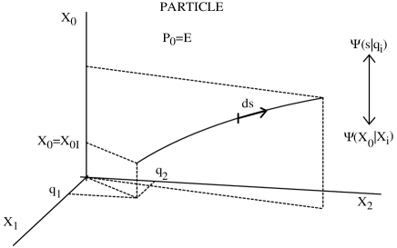
Figure 1: The world line $[s]$ of a relativistic particle in the space of events [$X_{0}|X_{i}$] with the initial data [$X_{0I}|q_{I}$] treated as the point of creation of the particle.

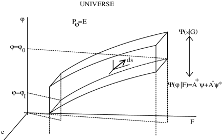
Figure 2: The world hypersurface [$s$] of the Universe in the space of events [$\varphi|F,e_{a\mu}$] with the vacuum initial data [$\varphi_{I}|G,e^{I}_{a\mu}$] treated as the point of creation of the Universe.

Expression (127) determining the probability of the creation of the world hypersurface in the space of events together with the geometric interval in a specific frame of reference solves the problems of the Dirac formulation dir ; fadpop : the nonlocalizable energy, arrow of time, comological singularity, and the initial data.

Faddeev and Popov proved in fadpop ; popkon that the integral (38) is not equivalent to the one in the relativistic invariant harmonic gauge $\partial_{\mu}(\sqrt{-g}g^{\mu\nu})=0$, which does not depend on a frame of reference. This means that the functional integral with the minimal surface (127) depends on the frame of reference, and the problem of relativistic invariance of the Hamiltonian formulation arises.

It is worthwhile to recall that the same problem arises also in SR, where in accordance with the theory of unitary irreducible representations of the Lorentz and Poincare groups the relativistic invariance means the invariance of a complete set of frames of reference with respect to the Lorentz transformations (see shwb ). In our case, the functional integral (127) should be repeated in each frame of reference of the complete set, so that the complete set of functional integrals with minimal surfaces is relativistic invariant.

IV Conclusion

We investigated General Relativity under the supposition that the evolution parameter of its Hamiltonian description coincides with the cosmological scale factor. The resulting Hamiltonian theory added by the vacuum postulate becomes free from the defects of the standard Hamiltonian approach and contains the cosmological Friedmann-like sector. The obtained Hamiltonian cosmological theory differs from the standard Lifshits-Bardeen cosmological perturbation theory lif ; bard ; kodam , where the cosmological scale factor is treated as an external field with the double counting of the spatial metric determinant. In contrast to the standard cosmological perturbation theory the Hamiltonian version contains the shift of the coordinate origin in the process of evolution, and the Newton-like form of interactions appears after resolving the constraints.

It is interesting to apply this cosmological Hamiltonian approach to GR for the description of the CMB fluctuations.

ACKNOWLEDGMENTS

We are grateful to D. Blaschke, A. Gusev, P. Flin, P. Fomin, L. Lipatov and D. Mladenov for fruitful discussions.

Appendix A: Field nature of time

To introduce the conformal time $\eta$ as a new field variable and its nonzero momentum as a proper energy of the geometric space of events, we can use the Levi-Civita-type canonical transformation bpp ; lc : $(P_{\varphi}|\varphi)\rightarrow(\Pi|\eta)$ to convert the energy constraint into a new canonical momentum $\Pi$. We consider this transformation using as an example the case of the Universe filled in by photons when $\rho_{0}(\varphi)=\mbox{\rm const.}$ In this case, this transformation takes the form

$$P_{\varphi}=\pm 2\sqrt{\Pi V_{0}},~{}~{}~{}~{}\varphi=\pm\frac{1}{2}\sqrt{\frac{\Pi}{V_{0}}}\eta.$$ (A.1)

The action (45) becomes

$$S_{c}=\int dx^{0}\left[-\Pi\partial_{0}\eta+N_{0}\left(\Pi-\rho_{0}V_{0}\right)\right].$$ (A.2)

After the reduction the non-zero energy $\Pi=V_{0}\rho_{0}$ corresponding to the invariant conformal time appears. The reduced action takes the form

$$S=V_{0}\int\limits_{\eta_{I}}^{\eta_{0}}d\eta\rho_{0}=V_{0}\rho_{0}(\eta_{I}-\eta_{0}).$$ (A.3)

In quantum theory, where $\Pi=d/id\eta$, the geometric evolution is described by the wave function

$$\psi_{\rm geometric}(\eta)=e^{iV_{0}\rho_{0}(\eta_{I}-\eta_{0})}.$$ (A.4)

The Hubble evolution $\varphi=\varphi(\eta)$ is treated as a pure relativistic effect of the relation between two supplementary descriptions of the relativistic Universe by means of two wave functions: the field (51) and the geometric (A.4) ones.

Appendix B: Central gravitational fields

Let us consider the central gravitational field produced by a single mass object

$$\overline{T}_{00}=M\left[\delta^{3}(x)-V_{0}^{-1}\right],~{}~{}\overline{T}_{kk}=0.$$ (B.1)

(see Eqs. (109), (110)). Equation (110) can be transformed into the integral form

$$\overline{\Phi}(x)=\frac{3}{4\pi\varphi^{2}}\left.\int d^{3}x\frac{T_{00}}{|y-x|}\right|_{T_{00}=M\delta^{3}(x)}=\frac{r_{g}}{r},$$ (B.2)

where $r=\sqrt{x_{1}^{2}+x_{2}^{2}+x_{3}^{2}}$ and

$$r_{g}=\frac{3M}{4\pi\varphi^{2}}=2GM;$$ (B.3)

here by definition $\varphi=\varphi_{0}a,~{}~{}M=M_{0}a$ and $\varphi_{0}=\sqrt{3/8\pi G}$.

In the case of $T_{kk}=0$, it follows from Eq. (109) that the shift vector $N_{i}$ is

$$N^{i}=\left(\frac{3r_{g}^{\prime}}{4}\right)\frac{x^{i}}{r}.$$ (B.4)

After substitution of the solutions (B.2) and (B.4) into the conformal interval we have

$$ds^{2}_{c}=\left(1-\frac{r_{g}}{r}\right)d\eta^{2}-\left(1+\frac{r_{g}}{r}\right)\left(dx_{i}+\frac{3}{2}\frac{x^{i}}{r}r^{\prime}_{g}d\eta\right)^{2};$$ (B.5)

here $ds^{2}_{c}=ds^{2}/a^{2}(\eta)$.

In the case of point mass distribution with the density

$$T_{00}=\sum_{I}M_{I}\delta^{3}(z_{I}-x)$$ (B.6)

the components of the metric $\overline{\Phi},~{}N^{i}$ are

$$\overline{\Phi}(x)=\sum^{N}_{I=1}\frac{r_{gI}}{|x-z_{I}|}$$ (B.7)

$$N^{i}=\sum^{N}_{I=1}\frac{3r_{gI}^{\prime}}{4}\frac{(x-z_{I})^{i}}{|x-z_{I}|}$$ (B.8)

The conformal interval

$$ds^{2}_{c}=(1-\overline{\Phi})d\eta^{2}-(1+\overline{\Phi})(dx^{i}+N^{i}d\eta)^{2}$$ (B.9)

determines an equation for the photon momenta

$$p_{\mu}p_{\nu}g^{\mu\nu}\simeq(p_{0}+N^{i}p^{i})^{2}(1+\overline{\Phi})-p^{2}_{j}(1-\overline{\Phi})=0,$$ (B.10)

from which we obtain

$$p_{0}\simeq-N^{i}p^{i}+(1-\overline{\Phi})|p|;~{}~{}~{}~{}~{}~{}~{}|p|=\sqrt{p^{2}_{i}}.$$ (B.11)

Finally, we obtain the relative magnitude of spatial fluctuations of a photon energy in terms of the metric components (the potential $\overline{\Phi}$ and shift function $N^{i}$)

$$\frac{p_{0}-|p|}{|p|}=-(N^{i}n^{i}+\overline{\Phi});~{}~{}~{}~{}~{}~{}~{}~{}~{}n^{i}=\frac{p_{i}}{|p|}.$$ (B.12)

The appearance of spatial anisotropic fluctuations of the photon energy in the flow of photons is the consequence of the minimal surface (B.4).

References

• (1) P. A. M. Dirac, Proc. Roy. Soc. A 246, 333 (1958); Phys. Rev. 114, 924 (1959).
• (2) R. Arnowitt, S. Deser, and C .W. Misner, Phys. Rev. 116, 1322 (1959); Phys. Rev. 117, 1595 (1960); Phys. Rev. 122, 997 (1961).
• (3) P. Bergman, Rev. Mod. Phys. 33, 510 (1961).
• (4) J. Schwinger, Phys. Rev. 130 1253 (1963); Phys. Rev. 132, 1317 (1963).
• (5) L.D. Faddeev and V.N. Popov, Us.Fiz.Nauk 111, 427 (1973).
• (6) J. A. Wheeler, Lectures in Mathematics and Physics (Benjamin, New York, 1968); B. C. DeWitt, Phys. Rev. 160, 1113 (1967).
• (7) C. Misner, Phys. Rev. 186, 1319 (1969).
• (8) M. P. Jr. Ryan, L. C. Shapley, ( Homogeneous Relativistic Cosmologies (Princeton Series on Physics, Princeton University Press, Princeton, 1975).
• (9) M. P. Ryan, Hamiltonian Cosmology (Lecture Notes in Physics N 13, Springer Verlag, Berlin–Heidelberg–New York, 1972).
• (10) E.M. Lifshits, Us.Fiz.Nauk 80, 411 (1963), in Russian; Adv. of Phys. 12, 208 (1963).
• (11) J.M. Bardeen, Phys. Rev. D22, 1882 (1980).
• (12) H. Kodama, M. Sasaki, Prog. Theor. Phys., N 78, 1 (1984).
• (13) V.A. Fock, Zs.f.Phys. 57, 261 (1929).
• (14) A.B. Borisov, V.I. Ogievetsky, Teor. Mat. Fiz., 21, 329 (1974).
• (15) A.L. Zel’manov, Doklady AN SSSR 227, 78 (1976), in Russian; Yu.S. Vladimirov, Frame of references in theory of gravitation (M., Energoizdat, 1982), in Russian.
• (16) N.P. Konoplyova, V.N. Popov, Kalibrovochnye polya (M. Atomizdat, 1980), in Russian.
• (17) See the review of papers by V. Bargman, E.P. Wigner, and A.S.Wightman in the monography by S. Schweber, Chapter 1, §1, 4, 5. An Introduction to Relavistic Quantum Field Theory (Row, Peterson and Co. Evanston, III., Elmsford, N.Y. 1961).
• (18) The proper time $ds=e_{(1)}d\tau$ becomes dynamical variables in the geometric space of events $[s|q_{i}]$ obtained by the Levi-Civita transformations $(p_{\mu}|x_{\mu})\Rightarrow(\Pi_{\mu}|s,q_{i})$, so that the constraint $p_{\mu}p^{\mu}-m^{2}=0$ becomes the new momentum $\Pi_{0}=0$ pp ; bpp ; lc ; sh ; gkp1 ; gkp .
• (19) M. Pawlowski, V.N. Pervushin, Int. J. Mod. Phys. 16, 1715 (2001); [hep-th/0006116].
• (20) B.M. Barbashov, V.N. Pervushin, M. Pawlowski, Phys. Particles and Nuclei 32, 546 (2001).
• (21) H. Poincare, C.R. Acad. Sci., Paris 140, 1504 (1905).
• (22) A. Einstein, Anal. d. Phys. 17, 891 (1905).
• (23) V.N. Pervushin, V.I. Smirichinski, J. Phys. A: Math. Gen. 32, 6191 (1999).
• (24) T. Levi-Civita, Prace Mat.-Fiz. 17, 1 (1906).
• (25) S. Shanmugadhasan, J. Math. Phys 14, 677 (1973).
• (26) S.A. Gogilidze, A.M. Khvedelidze and V.N.Pervushin, J. Math. Phys. 37, 1760 (1996); S.A. Gogilidze, A.M. Khvedelidze and V.N. Pervushin, Phys. Rev. D 53, 2160 (1996).
• (27) S.A. Gogilidze, A.M. Khvedelidze and V.N. Pervushin, Phys. Particles and Nuclei 30, 66 (1999).
• (28) E. Kasner, Am. J. Math 43, 217 (1921).
• (29) V.A. Belinsky, E. M. Lifshits, I.M. Khalatnikov, Us. Fiz. Nauk 102, 463 (1970), in Russian; JETF 60, 1969 (1971), in Russian; L.D. Landau, E.M. Lifshits, The theoretical  physics, V. 2. The field theory (M., Nauka, 1988).
• (30) D. B. Blaschke, S. I. Vinitsky, A. A. Gusev, V .N. Pervushin, and D. V. Proskurin, Physics of Atomic Nuclei 67, 1050 (2004); [gr-qc/0103114].
• (31) B. M. Barbashov, V .N. Pervushin, and D. V . Proskurin, Phys. of Particles and Nuclei, 34, Suppl. l, S68 (2003).