• The Chemical Composition of Alpha Centauri A: Strong Lines and the ABO Theory of Collisional Line Broadening

  M. T. Doyle^A,C, B. J. O’Mara (deceased¹), J. E. Ross^A,and M. S. Bessell^{B
  A} Physical Department, University of Queensland, St. Lucia, Qld 4072, Australia
  ^B RSAA, ANU, Mount Stromlo, Cotter Road, Weston Creek, ACT 2611, Australia
  ^C Email: mtdoyle@physics.uq.edu.au

  Abstract The mean abundances of Mg, Si, Ca, Ti, Cr and Fe based on both strong and weak lines of Alpha Centauri A are determined by matching the observed line profiles with those synthesized from stellar atmospheric models and comparing these results with a similar analysis for the Sun. There is good agreement between the abundances from strong and weak lines.

  Strong lines should generally be an excellent indicator of abundance and far easier to measure than the weak lines normally used. Until the development of the Anstee, Barklem and O’Mara theory for collisional line broadening, the uncertainty in the value of the damping constant prevented strong lines being used for abundance determinations other than in close differential analyses.

  We found that Alpha Centauri A has a mean overabundance of 0.12$\pm$0.06 dex compared to solar mean abundances. This result agrees remarkably well with previous studies that did not use strong lines or the Anstee, Barklem and O’Mara theory for collisional line broadening. Our result support the conclusion that reliable abundances can be derived from strong lines provided this new theory for line broadening is used to calculate the van der Waal’s damping.

  Keywords: stars: abundances, stars: individual (Alpha Centauri A), Sun: abundances

1 Introduction

The Alpha Centauri system has a special fascination for astrophysicists because it is the closest stellar system and its principle component, Alpha Centauri A ($\alpha$ Cen A), has a spectral type very similar to the Sun, G2V. $\alpha$ Cen A is also one of the brightest stars in the sky enabling spectra with a high spectral resolution and high signal to noise to be obtained. Most past analyses have concluded that the metal abundance of $\alpha$ Cen A is greater than that of the Sun. Analyses, such as Furenlid & Meylan (1990) covering 26 elements from 500 lines and Neuforge-Verheecke & Magain (1997) investigating 17 elements, concluded that the average metal overabundance compared to the Sun is 0.12$\pm$(0.02-0.04) dex and 0.24 dex respectively. Another study, Chmielewski et al. (1992), concluded that $\alpha$ Cen A can be classed as a super metal rich star.

The importance of the present study is the use of the Anstee, Barklem, and O’Mara theory (ABO theory, Barklem et al. (1998a) ) to determine van der Waal’s damping (VDW) for collisional line broadening for $\alpha$ Cen A. The ABO theory provides precise theoretical damping constants (as demonstrated in recent results for the analysis of strong lines in the solar spectrum by Allende Prieto et al.(2001)), which enables the use of strong lines for which reliable laboratory f-values exist. Strong line wings are also relatively insensitive to the effects of turbulence in the atmosphere. Thus strong line wings, together with the ABO theory, may be used as reliable abundance indicators for elements where such strong lines exist.

The choice of lines for this project follows Allende Prieto et al.(2001) investigation for the Sun and includes weak neutral, weak ionised, and strong lines for six elements, Mg, Ca, Si, Ti, Cr, and Fe.

We employ high quality coude echelle CCD spectra observed using the 74 inch telescope at Mt. Stromlo Observatory. The mass, distance, luminosity, and colours of $\alpha$ Cen A are used to determine its effective temperature, $T_{eff}$, and surface gravity, log($g_{s}$) necessary to customise existing atmospheric models to match $\alpha$ Cen A. The model is based on Kurucz solar models, (Kurucz 1979). The customised model, along with relevant atomic data, are used to synthesize line profiles for $\alpha$ Cen A. Abundances are determined by matching the observed profiles, following determination of turbulence parameters. Steps are taken to verify the $\alpha$ Cen A model used. A solar model based on the Holweger-Müller model (Holweger & Müller 1974) is used to synthesize line profiles which are matched to the observational line profiles from the Jungfraujoch Atlas (Delbouille & Roland 1995) to determine the solar mean abundance. The solar and $\alpha$ Cen A mean abundances are compared to find the mean under- or overabundance for $\alpha$ Cen A.

2 ABO Collisional Line Broadening Theory

Collisional or VDW broadening is broadening resulting from the collision of atoms in the photosphere. It is especially important in cool stars such as our Sun and $\alpha$ Cen A that have predominately neutral hydrogen photospheres. This collisional broadening produces a Lorentzian line profile. The damping constant for collisional broadening is $\Gamma_{coll}$ and is included when synthesizing the line profiles.

As discussed in Barklem et al. (1998a), up until the 1970’s, formulations of VDW broadening developed by Lindholm, Foley, and Ünsold were used and it was widely held that a better theory was needed. These theories deal with VDW interactions between perturbing hydrogen atoms and the absorbing atom. Although the term van der Waal’s broadening is still used today, it is really a misnomer as the actual line broadening theory is much more complex.

K.A. Brueckner (Brueckner 1971) introduced a perturbation theory formulation that involved long range interaction where the electron exchange could be neglected but not the overlap in the atomic charge distribution, a point taken up in O’Mara (1976). O’Mara’s work deals with collision broadening theory and draws on work from many sources to develop the beginning of what has come to be known as the ABO theory of line broadening. This theory has been further developed by Anstee, Barkelm and O’Mara (Anstee & O’Mara 1991, 1995; Barklem & O’Mara 1997; Barklem et al. 1998b). Further development of the ABO theory and its relevances to solar and late-type star abundances is on-going with a code available on the world wide web (Barklem et al. 1998a) to calculate VDW.

3 Observation and Data Reduction

Our spectra are taken on three separate observational runs in 1996 June/July and 2001 May on the 74 inch telescope at Mt Stromlo Observatory. The 120 inch focal length coude camera is used with a 31.6 groove/mm echelle, cross dispersed with a 150 lines/mm grating. Several different wavelength settings of the echelle grating and cross-disperser gratings are used to obtain almost complete wavelength coverage from 4000-8000 $\AA$.

The signal to noise ratio (S/N) varied with order across the CCD because of vignetting resulting from the cross-disperser not being near a pupil. The CCD has a gain of 2 electrons per ADU and most of the exposures are aimed at about 60000 electrons maximum. As the data are 60000-180000 electrons per resolution element, the nominal S/N ratio is 200-400. The actual resolution was 125000 estimated by measuring the width (FWHM) of the line at wavelength 8252.379 $\AA$ from the thorium arc spectrum:

$$R=\frac{\lambda}{\Delta\lambda}$$ (1)

which corresponds to a velocity of 2.392 km s^-1.

The reduction process includes cleaning the raw spectra of cosmic rays and flat fielding. The spectral orders are extracted and any scattered light between the orders is removed. Extracted spectra from a nearby “smooth spectrum” star $\beta$ Centauri, are divided through the spectra of the target star, $\alpha$ Cen A to eliminate telluric (Earth’s atmosphere) lines. An Th arc spectrum is used for wavelength calibration purposes. The spectra are smoothed to reduce noise and the continuum level is flattened. The wavelengths are also corrected for the radial velocity of $\alpha$ Cen A.

4 The Atmospheric Models and Line Profiles

Line profiles are synthesised for each line of interest and used to determine the abundances by fitting to the observed line profiles. Parameters such as macro and microturbulence, VDW damping, energy levels of the transitions, log gf values, and starting abundances are input to enable this direct matching process.

Two models and subsequent line profiles are used for $\alpha$ Cen A. Model AK is an interpolated Kurucz model (Kurucz 1979) grid; model AH is a scaled Holweger & Müller solar model (Holweger & Müller 1974). Both models use the calculated values for $\alpha$ Cen A’s effective temperature and surface gravity. These two models are compared to verify the validity of using the interpolated Kurucz model in this project.

The third model SH is the Holweger & Müller model (Holweger & Müller 1974). This is used to synthesize line profiles to fit observed solar data obtained from the Jungfraujoch Atlas.

The initial models based on published solar abundances, are used to compute line profiles to be compared with observations. If the line does not fit, the abundance of the element is adjusted and new number densities, opacities, and pressures are computed for a second iteration. This process is iterated to convergence yielding an abundance for each line. The temperature structure, $T_{log\,\tau}$, of the initial atmosphere is not adjusted.

4.1 Input Parameters and Calculations for the $\alpha$ Cen A Model Atmosphere and Synthesised Line Profiles

4.1.1 Effective Temperature and Surface Gravity

The parameters, effective temperature, $T_{eff}$, and surface gravity, log($g_{s}$), used to calculate the atmospheric model are very important.

In Table 1 we list the measurements and derived data for $\alpha$ Cen A and the Sun that are used to determine the surface gravities and effective temperatures and are computed using the following equations:

$$\log\,g_{s}=\log\,\left(\frac{Gm}{r^{2}}\right)$$ (2)

$$T_{eff}=\left(\frac{L}{4\pi r^{2}\sigma}\right)^{\frac{1}{4}}$$ (3)

The derived values are in close agreement with those researched by other authors and are listed in Table 2. For $\alpha$ Cen A the resulting values are $T_{eff}$=5784$\pm$5K and log($g_{s}$)=4.28$\pm$0.01.

Table 1: Researched and Calculated* values used to customise the model atmosphere and produce synthesised line profiles for $\alpha$ Cen A’s and the Sun

Parameters	$\alpha$ Cen A	Source	Sun	Source
Angular Diameter (arc sec)	$\left(86.2\pm 2.3\right)\times 10^{-4}$${}^{(\textrm{1})}$	Absolute IR photometry
Parallax (arc sec)	0.74212$\pm$0.0014${}^{(\textrm{2})}$	Hipparcos Catalogue
Apparent Magnitude V	-0.01$\pm$0.006${}^{(\textrm{2})}$	Hipparcos Catalogue	-26.74$\pm$0.06(3)	See Reference
Mv	4.35$\pm$0.006*	Section 4.1.2	4.83$\pm$0.002*	Section 4.1.2
Distance Modulus	-4.36$\pm 0.008$*	Section 4.1.2	-31.57$\pm$0.06*	Section 4.1.2
Bolometric Correction	-0.07$\pm$0.01${}^{(\textrm{4})}$	Observational & synthetic V band spectra	-0.07$\pm$0.01${}^{(\textrm{4})}$	Observational & synthetic V band spectra
Bolometric Magnitude	4.2755$\pm$0.01*	Calculated	4.7620$\pm$0.01*	Section 4.1.2
Mass (kg)	(2.1591$\pm$0.019)$\times 10^{30}$*	Section 4.1.2	1.99$\times 10^{30}$${}^{(\textrm{3})}$⋄	See Reference
Mass⊙	1.085$\pm$0.01(5)	From Models	1
Radius (m)	(8.6879$\pm 0.017$)$\times 10^{8}$*	Section 4.1.2	(6.96$\pm$0.00026)$\times 10^{8}$${}^{(\textrm{3})}$	See Reference
Radius⊙	1.2483$\pm$0.0024*	Section 4.1.2	1
Distance (m)	4.1578$\pm$0.0078$\times 10^{16}$*	Section 4.1.2	1.496$\times 10^{11}$ ${}^{(\textrm{3})}$⋄	See Reference
Distance (Parsecs)	1.3456$\pm$0.0025*	Section 4.1.2	4.848$\times 10^{-6}$* ⋄	Section 4.1.2
Luminosity (W)	6.0205$\pm$1$\times 10^{26}$*	Section 4.1.2	3.846$\times 10^{26}$ ${}^{(\textrm{3})}$⋄	See Reference
$\frac{L}{L_{\odot}}$	1.57$\pm$0.3*	Section 4.1.2	1
Surface Gravity (ms-2)	(1.901$\pm$0.019)$\times 10^{4}$*	Section 4.1.2	(2.74$\pm$0.0002)$\times 10^{4}$*	Section 4.1.2
Log gs	4.28$\pm$0.01*	Section 4.1.2	4.44$\pm$0.00003 *	Section 4.1.2
Effective Temperature (K)	5784.3$\pm$5.5*	Section 4.1.2	5778$\pm$1${}^{(\textrm{3})}$	See Reference

${}^{(\textrm{1})}$Blackwell & Shallis 1977; ${}^{(\textrm{2})}$Perryman 1997; ${}^{(\textrm{3})}$Ahrens 1995; ⁽⁴⁾Bessell et al. 1998; ${}^{(\textrm{5})}$Demarque et al. 1986, * calculated, ^⋄ error insignificant

Table 2: Comparing parameters for $\alpha$ Cen A from reviewed and this paper

Ref.	Teff(K)	log(g${}_{\textrm{s}}$)	$\xi$(km s-1)	Mv	$\frac{L}{L_{\odot}}$	$\frac{r}{r_{\odot}}$	$\frac{m}{m_{\odot}}$	$\Delta\log(A)$(dex)
${}^{\textrm{1}}$	5784.3$\pm$5.5	4.28$\pm$0.01	1	4.35$\pm$0.006	1.57$\pm$0.3	1.25$\pm$0.0024	1.085$\pm$0.01	0.12$\pm$0.06
2	5770$\pm$20					1.23
3	5710$\pm$25	4.0$\pm$0.2	1.0$\pm$0.2	4.38		1.26	1.085	0.12$\pm 0.06$
4	5765$\pm$50				1.53		1.085	0.25$\pm$0.02
5	5800$\pm$20	4.31$\pm 0.02$	1	4.374$\pm$0.01			1.085
6	5830$\pm 30$	4.30$\pm$0.03	1.09$\pm 0.11$		1.53		1.085$\pm 0.01$

${}^{(\textrm{1})}$This paper; ${}^{(\textrm{2})}$Soderblom 1986; ${}^{(\textrm{3})}$Furenlid & Meylan 1990; ⁽⁴⁾Noels et al. 1991; ${}^{(\textrm{5})}$Chmielewski et al. 1992; ${}^{(\textrm{6})}$Neuforge-Verheecke & Magain 1997.

4.1.2 Input Data for Line Profile Synthesis

The input data required for line synthesis are the energy levels, log(gf), and VDW parameters taken from Allende Prieto et al. (2001) (Tables 3 & 4), and the starting solar abundances from Grevesse & Sauval (1998) (Table 5).

The parallax ($\pi$) and angular diameter ($\theta$) are used to calculate $\alpha$ Cen A’s radius:

$$d=\frac{(d_{\odot})}{\pi}$$ (4)

$$r=\frac{[d(\theta/3600)(\pi/180)]}{2}$$ (5)

The apparent magnitude is used to calculate the effective temperature with the following steps:

$$M_{v}=V-5\log\frac{d}{10}$$ (6)

$$M_{bol}=M_{v}+BC$$ (7)

$$L=L_{\odot}10^{\left(\frac{M_{Bol\odot}-M_{Bol}}{2.5}\right)}$$ (8)

$$T_{eff}=\left(\frac{L}{4\pi r^{2}\sigma}\right)^{\frac{1}{4}}$$ (9)

4.2 Non-thermal Broadening Parameters

The non-thermal motions or turbulence that occur on a large scale compared with optical depth, is macroturbulence, and on the small scale is microturbulence.

Macroturbulence

Macroturbulence will broaden the line profile but does not affect the line strength (equivalent width). The effects of stellar rotation (small) and instrumental profile are included as enhancements to the macroturbulence.

Several single lines and one blend of lines are chosen to determine the effective macroturbulence. Various values are tested on each single line to see if a common value can be used to match the general shape of the observed line. When the value for the effective macroturbulence is determined, that value is used on the blended lines with no affect on the equivalent width of the synthesised line profile.

The $\alpha$ Cen A value for the effective macroturbulence is determined to be 3.3 km s^-1. This includes 2.4 km s^-1 due to instrumental effects and an atmospheric macroturbulence of 2.3 km s^-1. This indicates that most of the observed line broadening effects near the line core are from the large scale motions in the photosphere. Natural, Stark, and rotational broadening are insignificant for the lines chosen for this study.

The effective macroturbulence to match the solar model AH’s line profiles to the observed solar data is 1.6 km s^-1.

Microturbulence

Values for the microturbulence are determined by using weak neutral, weak ionised, and strong Fe lines. The values fitted are 1.08$\pm$0.2 km s^-1 for $\alpha$ Cen A with the AK model and 0.85 km s^-1 for the Sun using the SH model.

4.3 Validity of the Model

To judge whether the interpolated model AK is valid, comparison with an empirical model based on observations is useful.

The equivalent widths and profiles from model AK are compared to those produced with model AH a scaled solar empirical Holweger & Müller model (Holweger & Müller 1974).

Eight lines are chosen and a good match of line profiles and equivalent widths are obtained.

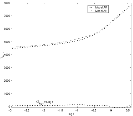
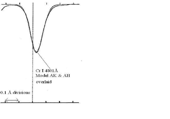
Another method for comparing the validity of model AK is to plot $T_{log\,\tau}$ vs. log$\tau_{o}$ for both models. As can be seen from Figure 1 there is close agreement for log$\tau_{o}$ -3-+0.6. This is the range of optical depths that are covered in this research. A direct comparison can be seen in Figure 2 where a strong line, CrI at 4801$\AA$, for both models have been overlaid and match exactly.

Figure 1: Temperature vs. Optical Depth. Comparison of the AK and AH Models to test for for validity.

Figure 2: Model AK & AH line profiles overlaid for CrI 4801 $\AA$

5 Analysis

5.1 Determining the Mean Abundance

Fitting the shape of the synthesised line profiles from model AK against that of the observations is straightforward for most of the lines.

For all lines, care is taken to ensure that the area of the synthesised and observed line profiles are equivalent, allowing for differences in the exact matching of the line profile’s core and wings. For two very weak lines and all the strong lines, extra care is needed.

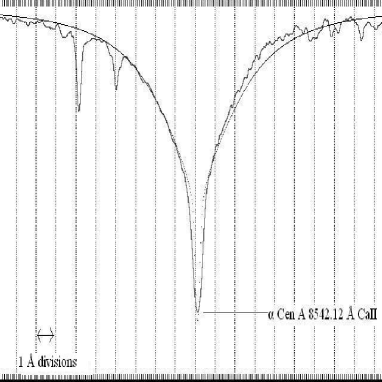
In the case of the strong lines, the core and wings cannot be matched simultaneously. In this case, the wings are matched, as per the ABO theory, and the core of the model’s line profile is extended as low as possible. Care is taken that this technique is followed in both model’s line profiles for those lines affected.

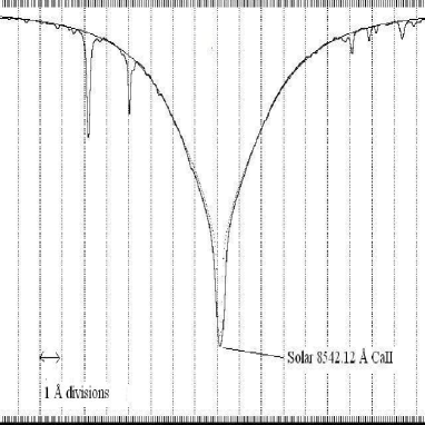
As can be seen in Figure 3 the right hand wing of the line profile for the observed data for $\alpha$ Cen A is higher than that of the synthesised line profile. This does not happen in the Sun’s line profile. The problem then is with the reduction process. Care is taken to ensure that features like this are compensated for in the determination of the abundances.

Figure 3: Fitting Model line profile to Observed Data for $\alpha$ Cen A and Sun to determine equivalent width and abundance for Strong CaII line 8542.120 $\AA$ (Scale: 1 divisions)

5.2 Results

The mean abundances are determined from 1 Mg, 7 Ca, 9 Si, 13 Ti, 6 Cr, and 22 Fe lines. Each element is represented by species that cover weak neutral, weak ionised, and strong lines except for Mg that is represented by one strong line. $\alpha$ Cen A shows a mean overabundance of 0.12$\pm$0.06 dex. The error is calculated from the variations in the individual species abundances.

These abundances are larger than those used for starting abundances from Grevesse & Sauval (1998). The individual equivalent widths ($W_{\lambda}$), abundance (A), and $\Delta$ abundances ($\Delta$A) for $\alpha$ Cen A and the Sun are listed in Tables 3 and 4. The mean abundance ($\left\langle A\right\rangle$), the $\Delta$ mean abundances ($\Delta$$\left\langle A\right\rangle$) along with the starting abundances for $\alpha$ Cen A and the Sun for each element and the final mean overabundance are listed in Table 5.

Table 3: Input Parameters and Abundances for $\alpha$ Cen A and the Sun

$\lambda$				VDW (2)		$\alpha$ Cen A (1)		Sun (1)		$\Delta$$\left\langle A\right\rangle$(1)
($\AA$)	Species(2)	E${}_{\textrm{low}}$(2)	log(gf)(2)	$\sigma$	$\alpha$	Wλ (m$\AA$)	A	Wλ (m$\AA$)	A	(dex)
4508.287	FeII	2.84	-2.520	188	0.267	109.53	7.935	90.59	7.670	0.027
4602.006	FeI	1.61	-3.150	296	0.260	91.08	7.870	73.68	7.680	0.190
4656.979	FeII	2.88	-3.580	190	0.330	36.80	7.346	31.97	7.330	0.016
4758.122	TiI	2.25	0.481	326	0.246	54.95	5.027	43.46	4.950	0.077
4759.274	TiI	2.25	0.570	327	0.246	57.32	4.990	47.90	4.958	0.032
4798.535	TiII	1.08	-2.670	211	0.209	54.95	5.130	41.77	5.000	0.130
4801.028	CrI	3.12	-0.131	348	0.240	59.73	5.800	49.66	5.720	0.800
4964.931	CrI	0.94	-2.527	262	0.291	49.04	5.790	35.90	5.720	0.700
5113.445	TiI	1.4	-0.727	298	0.243	36.10	5.003	25.15	4.950	0.053
5225.533	FeI	0.11	-4.790	207	0.253	86.83	7.823	71.07	7.680	0.143
5232.952	FeI	2.94	-0.058	713	0.238	382.43	7.450	376.95	7.510	-0.060
5234.632	FeII	3.21	-2.230	188	0.268	105.42	7.813	89.23	7.570	0.243
5247.057	FeI	0.09	-4.950	206	0.253	76.63	7.678	64.17	7.630	0.048
5272.002	CrI	3.45	-0.422	757	0.238	35.43	5.820	21.92	5.630	0.190
5295.781	TiI	1.05	-1.57	278	0.253	18.13	5.017	11.60	4.990	0.027
5300.751	CrI	0.98	-2.129	329	0.263	71.50	5.890	54.71	5.720	0.170
5312.859	CrI	3.45	-0.562	751	0.238	27.21	5.776	18.75	5.680	0.96
5336.793	TiII	1.58	-1.630	272	0.314	90.84	5.300	73.21	5.050	0.250
5418.773	TiII	1.58	-2.110	270	0.315	61.42	5.140	47.55	4.980	0.160
5490.154	TiI	1.46	-0.877	374	0.262	28.78	4.984	19.64	4.945	0.39
5665.557	SiI	4.92	-1.940	1772	0.222	56.34	7.680	39.12	7.480	0.200
5684.490	SiI	4.95	-1.550	1798	0.221	77.74	7.610	66.87	7.500	0.110
5690.425	SiI	4.93	-1.770	1772	0.222	62.79	7.616	52.84	7.520	0.096
5701.106	SiI	4.93	-1.950	1768	0.222	55.19	7.680	39.91	7.510	0.170
5708.402	SiI	4.95	-1.370	1787	0.222	95.29	7.640	84.96	7.537	0.103
5787.922	CrI	3.32	-0.083	1097	0.291	87.12	6.203	48.17	5.660	0.543
5866.457	TiI	1.07	-0.784	259	0.262	59.83	5.120	43.38	4.980	0.140
5916.254	FeI	2.45	-2.990	341	0.238	64.02	7.710	52.80	7.650	0.060
5922.115	TiI	1.05	-1.410	313	0.242	28.10	5.065	17.82	5.000	0.065
5948.545	SiI	5.08	-1.130	1875	0.222	107.51	7.663	94.74	7.506	0.157
6082.715	FeI	2.22	-3.570	306	0.271	47.38	7.697	33.24	7.590	0.107
6092.799	TiI	1.89	-1.323	398	0.239	7.92	5.125	3.77	4.96	0.165
6151.623	FeI	2.18	-3.300	277	0.263	62.73	7.711	49.26	7.61	0.101
6161.297	CaI	2.52	-1.266	978	0.257	79.49	6.540	66.02	6.409	0.131
6162.183	CaI	1.89	-0.097	878	0.236	280.96	6.350	277.82	6.350	0
6166.441	CaI	2.52	-1.142	976	0.257	81.87	6.454	75.14	6.420	0.034
6173.342	FeI	2.2	-2.880	281	0.266	81.34	7.740	70.01	7.664	0.076
6200.321	FeI	2.61	-2.440	350	0.235	85.81	7.750	74.75	7.680	0.070
6258.109	TiI	1.44	-0.299	355	0.237	62.19	5.010	51.87	4.980	0.030
6297.801	FeI	2.2	-2.750	278	0.264	86.68	7.700	76.60	7.650	0.050

${}^{(\textrm{1})}$This paper; ${}^{(\textrm{2})}$Allende Prieto et al. 2001

Table 4: Input Parameters and Abundances for $\alpha$ Cen A and the Sun (Continued)

$\lambda$				VDW(2)		$\alpha$ Cen A(1)		Sun(1)		$\Delta$$\left\langle A\right\rangle$(1)
($\AA$)	Species(2)	E${}_{\textrm{low}}$(2)	log(gf)(2)	$\sigma$	$\alpha$	Wλ (m$\AA$)	A	Wλ (m$\AA$)	A	(dex)
6371.361	SiII	8.12	-0.000	389	0.189	43.34	7.850	35.22	7.520	0.330
6432.684	FeII	2.89	-2.510	174	0.270	53.76	7.600	43.42	7.449	0.151
6455.604	CaI	2.52	-1.290	365	0.241	69.90	6.490	56.85	6.350	0.140
6481.878	FeI	2.28	-2.980	308	0.243	76.78	7.757	65.20	7.680	0.077
6498.945	FeI	0.96	-4.700	226	0.253	57.82	7.740	43.20	7.658	0.082
6499.656	CaI	2.52	-0.818	364	0.239	101.06	6.600	92.17	6.500	0.100
6516.086	FeII	2.89	-3.380	174	0.270	45.07	7.270	53.99	7.550	-0.280
6750.161	FeI	2.42	-2.620	335	0.241	111.89	8.150	79.07	7.695	0.455
6978.861	FeI	2.48	-2.500	337	0.241	108.08	8.000	82.04	7.662	0.338
7357.735	TiI	1.44	-1.06	329	0.244	29.57	5.060	20.77	5.030	0.030
7515.836	FeII	3.9	-3.450	187	0.271	23.33	7.750	14.73	7.517	0.233
7680.271	SiI	5.86	-0.590	2107	0.495	101.18	7.640	101.78	7.610	0.030
7711.730	FeII	3.9	-2.450	186	0.264	58.42	7.560	50.79	7.430	0.130
7918.387	SiI	5.95	-0.510	2934	0.232	108.85	7.600	102.00	7.504	0.096
8327.067	FeI	2.20	-1.525	258	0.247	226.21	7.660	198.38	7.621	0.039
8542.120	CaII	1.7	-0.463	291	0.275	3206.68	6.360	3274.47	6.360	0
8662.169	CaII	1.69	-0.723	291	0.275	2568.95	6.420	2566.40	6.380	0.040
8806.778	MgI	4.33	-0.120	531	0.292	679.65	7.900	562.10	7.680	0.220

${}^{(\textrm{1})}$This paper; ${}^{(\textrm{2})}$Allende Prieto et al. 2001

Table 5: Mean Abundances and Mean Overabundances for $\alpha$ Cen A models (AK), and Sun Model (SH)

Element	Grevesse & Sauval 1998	$\alpha$ Cen A - $\left\langle A\right\rangle$	Solar - $\left\langle A\right\rangle$	$\Delta$$\left\langle A\right\rangle$ (dex)
Mg	7.58$\pm$0.05	7.9 (1 line)	7.6800	0.200
Ca	6.36$\pm$0.02	6.459$\pm$0.092	6.396$\pm 0.054$	0.064$\pm$0.017
Si	7.55$\pm$0.05	7.664$\pm$0.0756	7.521$\pm 0.0370$	0.144$\pm$0.011
Ti	5.02$\pm$0.06	5.075$\pm$0.088	4.983$\pm 0.032$	0.092$\pm$0.019
Cr	5.67$\pm$0.03	5.880$\pm$0.163	5.688$\pm$0.038	0.192$\pm$0.029
Fe	7.50$\pm$0.05	7.714$\pm$0.197	7.599$\pm 0.098$	0.115$\pm$0.029
$\alpha$ Cen A’s mean overabundance = 0.12$\pm$0.06 dex

6 Summary and Discussions

The mean abundance for the six elements investigated in the chemical composition of $\alpha$ Cen A are Mg=7.9 , Ca=6.46$\pm$0.09, Si=7.66$\pm$0.07, Ti=5.07$\pm$0.09, Cr=5.88$\pm$0.16, and Fe=7.71$\pm$0.20 dex. This leads to a mean abundance of 0.12$\pm$0.06 dex with respect to the Sun.

Previous studies are not able to use strong lines as no reliable theory existed to calculate the collisional broadening of these lines. For this project the development of the ABO theory (Barklem et al. 1998a) to calculate the VDW damping, enable us to use strong lines in determining the mean abundance of $\alpha$ Cen A compared to the Sun.

The $\alpha$ Cen A parameters used are $T_{eff}$=5784.3$\pm$5.5K and log($g_{s}$)=4.28$\pm$0.01. Two models for $\alpha$ Cen A are used, the second one (AH) a scaled solar model for comparison with the first (AK) to verify the validity of using an interpolated Kurucz model (Kurucz 1979). Once the use of model AK is validated, this model is used to synthesize line profiles for $\alpha$ Cen A to match the observed line profiles.

Solar abundances are determined from comparing observed line profiles from the Jungfraujoch Atlas with those of the Holweger-Müller solar model (Holweger & Müller 1974)).

The results of this study, that $\alpha$ Cen A is overabundant with respect to the Sun and can be included with other metal rich stars, agrees with those of previous studies (Noels et al. 1991; Chmielewski et al. 1992; Neuforge 1993; Neuforge-Verheecke & Magain 1997) with an exact agreement of mean overabundance of 0.12$\pm$0.06 dex by Furenlid & Meylan (1990). This mean overabundance indicates that $\alpha$ Cen A did not originate in the same cloud as the Sun but from material that is more enriched by stellar nuclear processing.

The above studies did not use strong lines or the ABO theory. Our result supports the determination that reliable abundances can be derived from strong lines provided the ABO theory is used to calculate the VDW damping.

By using the ABO theory for strong lines, the analysis of spectra, construction of model atmospheres, and the subsequent synthesised line profiles, the chemical composition of apparently faint stars, such as those in external galaxies can be determined. All galaxies contain cool F,G K type stars whose spectra contain strong metallic lines. Previously these lines were not able to be used for absolute abundances due uncertainties in the theory for calculating the VDW damping. With the ABO theory now firmly established and reliable model atmospheres existing for cool stars it will be possible to extend reliable abundance analyses to more and more distant galaxies using strong lines.

Acknowledgments

I would like to acknowledge and thank Paul Barklem for the use of the VDW damping values calculated from the ABO theory and the Astrophysics Group at the University of Queensland. I would also like to thank the anonymous referees for their constructive comments.

References

Ahrens T.J., ed.  1995, Global Earth Physics, a Handbook of Physical Constants

Allende Prieto C., Barklem P.S., Asplund M., Ruiz Cobo B., 2001, ApJ, 558, 830

Anstee S.D., O’Mara B.J., 1991, MNRAS, 253, 549

Anstee S.D., O’Mara B.J, 1995, MNRAS, 276, 859

Barklem P.S., Anstee S,D., O’Mara B.J., 1998a, PASA, 15, 336

Barklem P.S., O’Mara B.J., 1997, MNRAS, 290, 102

Barklem P.S., O’Mara B.J., Ross J.E., 1998b, MNRAS, 296, 1057

Bessell M. S., Castelli F., Plez B., 1998, AA, 333, 231

Blackwell D.E, Shallis M.J., 1977, MNRAS, 180, 177

Brueckner K.A., 1971, ApJ, 169, 621

Chmielewski Y., Friel E., Cayrel de Strobel G., Bentolila C., 1992, AA, 263, 219

Delbouille L., Roland C., 1995, ASP, 81,32

Demarque P., Guenther D.B., van Altena W.F., 1986, ApJ, 300, 773

Furenlid I., Meylan T., 1990, ApJ, 350, 827

Grevesse N., Sauval A.J., 1998, Space Science Review, 85, 161

Holweger H., Müller E.A., 1974, Solar Physics. 39, 19

Kurucz R.L., 1979, ApJS, 40, 1

Neuforge C., 1993, AA, 268, 650

Neuforge-Verheecke C., Magain P., 1997, AA, 328, 261

Noels A., Grevesse N., Magain P., Neuforge C., Baglin A., Lebreton Y., 1991, AA, 247, 91

O’Mara B.J., 1976, MNRAS, 177, 551

Perryman M.A.C., ESA, 1997, The HIPPARCOS and TYCHO Catalogues. Astrometric and Photometric catalogues derived from the ESA Hipparcos Space Astrometry Mission, ESA Publications Division, Netherlands, 1997, vol 1200

Soderblom D.R., 1986, AA, 158, 273