Mapping Substructures in Dark Matter Halos

Abstract

We present a detailed study of the real and integrals-of-motion space distributions of a disrupting satellite obtained from a fully self-consistent high-resolution cosmological simulation of a galaxy cluster. The satellite has been re-simulated using various analytical halo potentials and we find that its debris appears as a coherent structure in integrals-of-motion space in all models (“live” and analytical potential) although the distribution is significantly smeared for the live host halo. The primary mechanism for the dispersion is the mass growth of the host. However, when quantitatively comparing the effects of “live” and time-varying host potentials we conclude that not all of the dispersion can be accounted for by the steady growth of the host’s mass. We ascribe the remaining discrepancies to additional effects in the “live” halo such as non-sphericity of the host and interactions with other satellites which have not been modeled analytically.

1 Introduction

With the discovery of stellar streams within the Milky Way (e.g Helmi et al., 1999; Chiba & Beers, 2000; Ibata et al., 2002; Brook et al., 2003; Yanny et al., 2003; Navarro, Helmi & Freeman, 2004; Majewski et al., 2004) and M31 (e.g. Ibata et al., 2001; McConnachie et al., 2004) and streams and shells in clusters (e.g. Trentham & Mobasher, 1998; Gregg & West, 1998; Calcáneo-Roldán et al., 2000; Feldmeier et al., 2002) they have become a standard fixture in our understanding of galaxy and cluster formation. These streams provide important observational support for the hierarchical build-up of galaxies and clusters and the $\Lambda$-dominated cold dark matter ($\Lambda$CDM) paradigm. Future observational experiments such as RAVE and GAIA are designed to shed further light on the importance of streams in galaxy formation. Thus to better interpret this observational data coming online in the near future it is necessary to have clear theoretical understanding of the stellar streams left behind by dissolving satellites.

The most common approach to this has been to simulate the disruption of individual satellite galaxies in static analytical potentials representative of the distribution of dark matter (DM) halos (e.g. Kojima & Noguchi, 1997; Helmi & de Zeeuw, 2000; Harding et al., 2001; Ibata et al., 2002; Bekki et al., 2003; Majewski et al., 2004). Such simulations have provided great insight into the formation of stellar (e.g. Ibata et al., 2002) and gaseous (e.g. Yoshizawa & Noguchi, 2003; Connors et al., 2004) streams, and helped to constrain the shape of the Milky Way’s halo (e.g. Johnston et al., 1999; Ibata et al., 2001) and substructure content (e.g. Johnston et al., 2002).

The $\Lambda$CDM structure formation scenario predicts that small objects form first and subsequently merge to form entities thus DM halos are never “at rest” but always be in the process of accreting material from its vicinity and hence grow in mass. This also extends to the Milky Way, although it encountered its last major merger some 10 Gyrs ago (e.g. Gilmore, Wyse & Norris, 2003). Therefore, the question presents itself, is a static analytical DM potential a valid assumption for a study of the disruption of satellites?

While Zhao et al. (1999) already addressed the issue of the evolution of a satellite galaxy in a time-varying analytical potential, we are going to complement this study by comparing the disruption processes of satellite galaxies in analytical potentials and fully self-consistent cosmological simulations.

2 The Simulations

This study focuses on halo #1 from the series of high-resolution $N$-body galaxy clusters simulations (Gill et al., 2004a, c). Halo #1 was chosen because it is the oldest of the simulated clusters (i.e. 8.3 Gyrs) having a reasonably quiet merger history. The self-consistent cosmological simulations were carried out using the publicly available adaptive mesh refinement code MLAPM (Knebe, Green & Binney, 2001) in a standard $\Lambda$CDM cosmology ($\Omega_{0}=0.3,\Omega_{\lambda}=0.7,\Omega_{b}h^{2}=0.04,h=0.7,\sigma_{8}=0.9$). For a more details and an elaborate study of these simulations we refer to reader to Gill et al. (2004a, c).

From this simulation we chose one particular satellite galaxy orbiting within the live host halo and refer to its evolution as the “live model”. This choice was based upon two constraints: firstly, the satellite contains a sufficient number of particles and secondly, it has had multiple orbits. The satellite used throughout this study complies with these criteria in a way that it consists of $\sim$ 15,000 particles (as opposed to $\sim$ 800,000 for the host) at the “initial” redshift $z=1.16$ (8.3 Gyrs ago) and has roughly 4 orbits within the host’s virial radius until $z=0$ when the mass of the host reached $2.8\times 10^{14}$$h^{-1}{\ }{\rm M_{\odot}}$ (roughly 1,550,000 particles).

After extracting the satellite from the cosmological simulation we used a tree $N$-body code (GCD+: Kawata & Gibson, 2003) to model its evolution for 8.3 Gyrs in two (external) analytical potentials. The first of these two models we call the “evolutionary model” which uses an analytical reconstruction of the live halo’s potential as follows: at each available snapshot of the live model, we fitted the host’s DM density profile to the functional form of a (spherical) Navarro, Frenk & White profile (Navarro, Frenk & White, 1997, NFW):

$$\frac{\rho(r)}{\rho_{b}}=\frac{\delta_{s}}{(r/r_{s})(1+r/r_{s})^{2}}\ ,$$ (1)

where $\rho_{b}$ measures the cosmological background density, $\delta_{s}$ controls the amplitude and $r_{s}$ measures the radius where the profile turns from its logarithmic slope of $d\log\rho/d\log r=-1$ to $d\log\rho/d\log r=-3$. From this series of snapshot NFW profiles we reconstruct the evolution of the parameters $\delta_{s}(z)$ and $r_{s}(z)$. Our best fitting functions are given below:

$$\begin{array}[]{lcl}\delta_{s}&=&\displaystyle\frac{23456}{(z+0.08)^{0.28}}-1015\ ,\\ \\ r_{s}&=&167.28-58.14\ z^{1.2}\ .\\ \end{array}$$ (2)

Fig. 1 shows the evolution of $r_{s}$, $\delta_{s}$ and consequentially mass as a function of redshift for both the numerical simulation alongside the analytical formula described by equation (2). The increase of the host’s mass around $z=0.45$ is related to a transient (“backsplash”) satellite galaxy passing just within the virial radius at high velocity (cf. Gill, Knebe & Gibson, 2004b). The second model assumes a static analytical host potential and hence is labeled “fixed model”. The parameters $\delta_{s}=21070$ and $r_{s}=97.8$ adopted for the fixed model agree with the initial values for the evolutionary model. Note that in both analytical models the hosts are assumed to be spherical. Dynamical friction is not implemented, either.

Figure 1: The redshift dependence for $r_{s}$ (upper panel), $\delta_{s}$ (middle panel) and consequentially virial mass, $M_{\rm vir}$ (lower panel). The solid lines indicate the evolution in the live model, and the dashed lines are our best fitting formula to describe the evolution (see eq. 2).

3 The Results

In Fig. 2 we show the real-space distribution (left panel) of the disrupted satellite after the 8.3 Gyrs evolution, i.e. at $z=0$ along with its distance to the host as a function of time (right panel). The spread in the number of orbits amongst the models can readily ascribed to the difference in host mass and the small “mis-modeling” of its growth as seen in Fig. 1 at around redshift $z=0.3$.

This figure further highlights a number of interesting differences and similarities amongst the models. The most striking feature is that neither of the analytical models is capable of producing the real-space distribution of particles seen in the live model, and the live model shows the most “compact” distribution. Although all models display “shell”-like features, they are less eminent for the live host. Instead, the live model exhibits a “cross-like” feature and appears to be more compact in the central region, respectively. A comparable feature, in fact, has also been noted in observational streams (cf. Hau et al., 2004).

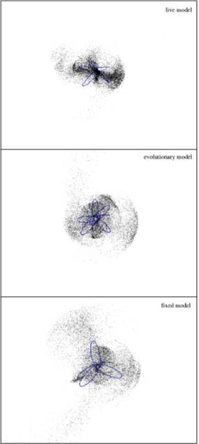
Figure 2: The projected particle distribution for all the models at $z=0$. The lines indicate the orbital paths of the satellite of the respective model.

Helmi & de Zeeuw (2000) outlined a method for identifying stellar streams within observational data sets by utilising conservation of energy, $E$, and angular momentum, $L$, (i.e. the integrals-of-motion) for spherically symmetric and time-independent potentials. In fact, this method proved to be a powerful tool for identifying streams in the Milky Way using the proper motions of solar neighbour stars (e.g. Helmi et al., 1999; Chiba & Beers, 2000; Brook et al., 2003; Navarro, Helmi & Freeman, 2004). We expand their analysis not only limiting ourselves to static analytical models but extending the study to include both our live and evolutionary models.

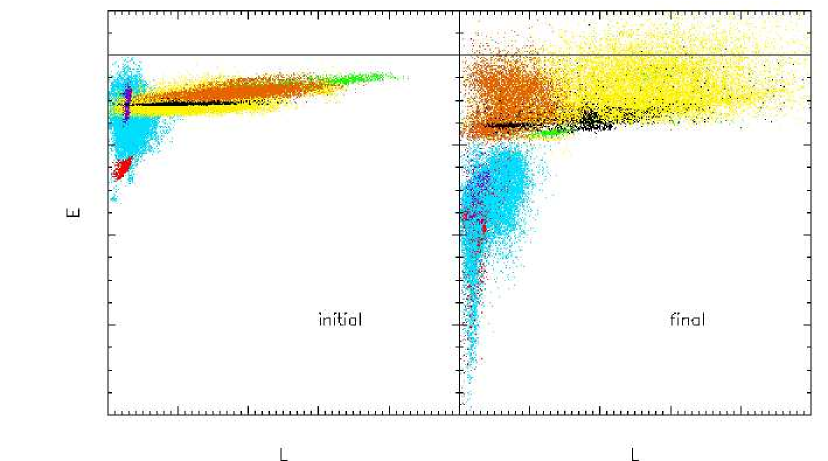
Figure 3: The distribution of satellite particles in the $E-L$ plane for the live models. The left panel shows the distributions at the time the respective satellite galaxy enters the virial radius of the host whereas the right panel presents the distributions at $z=0$. Different colours represent particles of different satellites.

Before exploring the evolution in the $E-L$ plane (hereafter also called “integral-space”) of our target satellite in all three models, we present the evolution for eight different satellites in the live model alone. The result can be viewed in Fig. 3 where each satellite is represented by an individual colour with our target satellite plotted as cyan. The satellites shown in Fig. 3 are all taken from the self-consistent cosmological simulation and represent a fair sample of all 158 available satellites, i.e. their masses cover a range from from $M\sim 5\times 10^{10}$$h^{-1}{\ }{\rm M_{\odot}}$ to $M\sim 4\times 10^{12}$$h^{-1}{\ }{\rm M_{\odot}}$ and they are on different orbits. The left panel of Fig. 3 shows the distributions at the time the satellite enters the virial radius of the host, whereas the right panel displays the distributions at $z=0$.

Fig. 3 allows us to gauge the “drift” of satellites in integral-space. We note that, compared to Fig. 4 of Helmi & de Zeeuw (2000), the integrals-of-motion are hardly conserved in the live model, neither for high or low mass streamers. The distributions rather show a large scatter, and have been significantly “re-shaped” over time. In addition, the mean values of $E$ and $L$ are also moved after the evolution. For instance, the “red” satellite drifts in time over to the initial position of the “cyan” satellite. Fig. 3 further demonstrates that the drift of our target satellite (cyan dots) is comparable to the evolution of the other satellites, thus indicating that this target satellite is a “typical satellite” in that respect.

One encouraging result implied from Fig. 3, however, is that even though the integrals-of-motion are changing over time, satellites still appear coherent in the $E-L$ plane. Hence, the integral-space analysis pioneered by Helmi & de Zeeuw (2000) still proves to be a useful diagnostic to identify streams. We further like to stress that observations only provide us with the snapshot of the distribution at today’s time, i.e. the right hand panel of Fig. 3 and hence measuring “evolution” is beyond the scope of RAVE and GAIA.

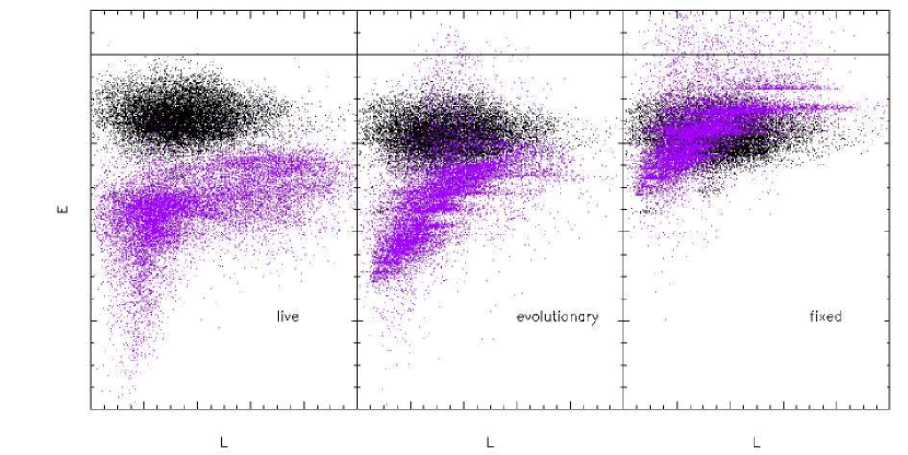
Figure 4: Total energy, $E$, versus absolute value of the angular momentum, $L$, for all satellite particles within the target satellite at initial redshift $z=1.16$ (black) and at $z=0$ (blue) in the live (left), evolutionary (middle) and fixed (right) models. The horizontal line indicates $E=0$.

Fig. 4 now focuses on our target satellite alone, showing its particles at initial and final time in the $E-L$ plane for all three models, i.e. the live, evolutionary and fixed model. We notice that particles tend to form “stripes” in the $E-L$ plane (parallel to the $L$-axis) indicative of a spread in angular momentum for particles of comparable energy. These stripes form over time and have been directly linked to both apo- and peri-centre passages of the satellite. The live model deviates most prominently from the other models not only reducing total energies, but also “randomising” the angular momentum and hence lacking the prominence of these stripes. We also observe in Fig. 4 that the fixed model is the only model to show a noticeable number of particles ($\approx$ 3%) not bound to the host halo, i.e. $E>0$. This can be ascribed to the lower mass of the host halo.

Moreover, Fig. 4 confirms the findings of Helmi & de Zeeuw (2000) that within a fixed host potential a satellite galaxies retains its identity in the $E-L$ plane and the integrals-of-motion hardly change, respectively. This statement is further strengthened by Fig. 5 which presents the actual frequency distribution of $E$ and $L$ at the initial and final time.

Not surprisingly, the live model shows the largest deviations from the initial configuration (Fig. 5). In the live model the distribution of $E$ and $L$ is broadened over time, and the peak of $E$ systematically moves toward lower values, while the peak of $L$ does not change dramatically for this particular satellite. This “drop” of $E$ is also observed in the evolutionary model; it reflects the steady mass growth and related deepening of the host potential (cf. Fig. 1). Since the drift in $E$ is the most significant change, the evolutionary model displays a similar distribution to the live model in the $E-L$ plane at $z=0$.

To further quantify the evolution of the satellite in integral-space, we calculate the centre and area of the particle distribution seen in Fig. 4 as a function of time. The centre is defined to be the two dimensional arithmetic mean in $E$ and $L$ values, respectively. The area covered in the $E-L$ plane is computed using a regular 128³ grid covering that plane from $L_{\rm min}$ to $L_{\rm max}$ and $E_{\rm min}$ to $E_{\rm max}$ in the respective model. Here, only cells containing more than three particles are taken into account. The evolution of both area and centre as a function of time since $z=1.16$ is presented in Fig. 6.

The top panel of Fig. 6 (showing the change in area) demonstrates that all three halos loose coherence of the distribution in integral-space. This loss is most prominent for the live model and least for the fixed model. This phenomenon can also be seen in a comparison between Fig. 4 of Helmi & de Zeeuw (2000) and the right panel of Fig. 3. Therefore, we conclude that a fixed (and even an evolutionary) model significantly underestimates the scatter in the integral-space, and earlier predictions based on the simulation using a static (or time-varying) analytical description for the halo potential overestimate their efficiency of the detection ability of streams.

The bottom panel of Fig. 6 (showing the drift of the distribution’s centre in the $E-L$ plane with respects to its initial position) is yet another proof that the fixed model holds the best conservation of energy and angular momentum. The “live” nature of the host mass can be held responsible for not only the increased dispersion (i.e. area) but also for the actual drift in integral-space. We further like to stress that at not time the evolutionary model matches the effects of the “live” model. There always appears to be a well pronounced discrepancy which can be ascribed to effects not considered in the evolutionary model, such as the triaxiality of the host and interactions of the debris with other substructure. This leads to the immediate conclusion that for an understanding of the formation of streams in integrals-of-motion space it appears rather crucial to take into account the full complex evolutioary effects of the host. The first such step has been taken by Zhao et al. (1999) who modeled the evolution of tidal debris in a time-varying potential. However, our study further indicates that in a “live” scenario there are additional effects at work leading to an even greater dispersion.

Figure 5: The distribution of energies (upper panels) at initial (black) and final (blue) time and angular momentum (lower panels) for the three models (live, evolutionary, fixed, from left to right).

Figure 6: The evolution of the area (top panel) and the centre (bottom panel) in integral-space (see text for more details) as a function of time for the live (solid), evolutionary (dot-dashed) and fixed (dotted line) models.

4 Conclusions

In hierarchical structure formation scenarios as favoured by recent estimates of the cosmological parameters (Spergel et al., 2003) DM halos continuously grow via both merger activity and steady accretion of material. Furthermore, they also contain a great deal of substructure and are far from spherical symmetry. We have investigated the development of streams due to the tidal disruption of satellite galaxies in a DM halo forming in a fully self-consistent cosmological simulation. This not only models the time-dependency of the potential (reflecting the mass growth of the host), it also accounts for other effects such as the triaxiality of the host and interactions of the debris with other satellites.

Our conclusions can be summarised as follows. (1) The distributions of (debris of) satellite galaxies in both real and integrals-of-motion space are sensitive to the evolution (and the particulars) of their host galaxy. This puts a caution on studies that investigate the shape of the halo based on satellite streams obtained via simulations with static DM halos. (2) Even in a $\Lambda$CDM “live” halo, satellites still appear to be coherent structures in the integrals-of-motion space. However, the coherency is smeared significantly in contrast to predictions from simulations using static and time-varying host potentials, respectively. Thus, earlier studies of the detection ability of streams using a static DM potentials (e.g. Helmi & de Zeeuw, 2000; Harding et al., 2001) and even time-varying potentials (Zhao et al. 1999) could overestimate the efficiency of the “integrals-of-motion approach”. (3) In the integrals-of-motion space, energy changes most significantly due to the mass growth of the host halo which is inevitable in hierarchical structure formation scenarios. However, there are additional effects at work such as triaxiality of the host and interactions of the stream with other satellites. Hence, any currently observed distribution of a satellite stream in the $E-L$ plane no longer reflects its original distribution.

5 Acknowledgments

The simulations presented in this paper were carried out on the Beowulf cluster at the Centre for Astrophysics & Supercomputing, Swinburne University. The financial support of the Australian Research Council is gratefully acknowledged. We also appreciate useful discussion with Chris Brook.

References

- Bekki et al. (2003) Bekki K., Couch W.J., Drinkwater M.J., Shioya Y., 2003, MNRAS, 344, 399
- Brook et al. (2003) Brook, C.B., Kawata, D., Gibson, B.K., Flynn, C., 2003, ApJ, 585, L125
- Calcáneo-Roldán et al. (2000) Calcáneo-Roldán C. Moore B., Bland-Hawthorn J., Malin D., Sadler E.M. 2000, MNRAS, 314, 324
- Chiba & Beers (2000) Chiba M., Beers T.C., 2000, AJ, 118, 2843
- Connors et al. (2004) Connors T.W., Kawata D., Maddison S.T., Gibson B.K., PASA, 21, 222
- Feldmeier et al. (2002) Feldmeier J.J., Mihos C., Morrison H.L. Rodney S., Harding P., 2002, ApJ, 575, 779
- Gardiner & Noguchi (1996) Gardiner L.T., Noguchi M., 1996, MNRAS, 278, 191
- Gill et al. (2004a) Gill S.P.D., Knebe A., Gibson B.K., 2004a, MNRAS, 351, 399
- Gill, Knebe & Gibson (2004b) Gill S.P.D., Knebe A., Gibson B.K., MNRAS, in press (astro-ph/0404427)
- Gill et al. (2004c) Gill S.P.D., Knebe A., Gibson B.K., Dopita M. A., 2004b, MNRAS, in press (astro-ph/0404255)
- Gilmore, Wyse & Norris (2003) Gilmore G., Wyse R.F.G., Norris J.E., 2003, ApJL, 574, 39
- Gregg & West (1998) Gregg M.D., West M.J. 1998, Nature, 396, 549
- Helmi & de Zeeuw (2000) Helmi A., de Zeeuw P.T., 2000, MNRAS, 319, 657
- Helmi et al. (1999) Helmi A., White S.D.M., de Zeeuw P.T., Zhao, H., 1999, Nature, 402, 53
- Harding et al. (2001) Harding P., Morrison, H.L., Olszewski E.W., Arabadjis J. Mateo M., Dohm-Palmer R.C., Freeman K.C., Norris J.E., ApJ, 122, 1397
- Hau et al. (2004) Hau G., Gill S.P.D., Knebe A., Gibson B.K., 2004 in preparation
- Ibata et al. (2001) Ibata R.A., Irwin M.J., Lewis G.F., Ferguson A.M.N., Tanvir N.R., 2001, Nature, 412, 49
- Ibata et al. (2001) Ibata R.A., Lewis G.F., Irwin M.J., Totten E., Quinn T., 2001, ApJ, 551, 294
- Ibata et al. (2002) Ibata R.A., Lewis G.F., Irwin M.J., Cambrésy L., 2002, MNRAS, 332,921
- Johnston et al. (1999) Johnston K.V., Zhao H., Spergel D.N., Hernquist L., 1999, ApJL, 512, 109
- Johnston et al. (2002) Johnston K.V., Spergel D.N., Haydn C., 2002, ApJ, 570, 656
- Kawata & Gibson (2003) Kawata D., Gibson B.K., 2003, MNRAS, 340, 908
- Knebe, Green & Binney (2001) Knebe A., Green A., Binney J., 2001, MNRAS, 325, 845
- Kojima & Noguchi (1997) Kojima M., Noguchi M., 1997, APJ, 481, 132
- Lokas & Mamon (2001) Lokas E.L., Mamon G.A., 2001, MNRAS, 343, 401
- Majewski et al. (2004) Majewski S.R., Kunkel W.E., Law D.R., Patterson R.J. Polak A.A. et al., 2004 AJ in press (astro-ph/0403701)
- McConnachie et al. (2004) McConnachie A., Irwin M., Lewis G., Ibata R., Chapman S., Ferguson A., Tanvir N., 2004 MNRAS in press (astro-ph/0406055)
- Navarro, Frenk & White (1997) Navarro J., Frenk C.S., White S.D.M., 1997, ApJ, 490, 493 (NFW)
- Navarro, Helmi & Freeman (2004) Navarro J.F., Helmi A., Freeman K.C., 2004, ApJ, 601, 43
- Spergel et al. (2003) Spergel D.N., Verde L., Peiris H.V., Komatsu E., Nolta M.R. et al., 2003, ApJS 148, 175
- Trentham & Mobasher (1998) Trentham N., Mobasher B., 1998, MNRAS, 293, 53
- Yanny et al. (2003) Yanny B., Newberg H.J., Grebel E.K., Kent S., Odenkirchen M. et al. 2003, ApJ, 588, 823
- Yoshizawa & Noguchi (2003) Yoshizawa A.M., Noguchi M., 2003, MNRAS, 339, 1135
- Zhao et al. (1999) Zhao H.S., Johnston K.V., Hernquist L., Spergel D.N., 1999, A&A 348, L49