Luminosity functions of Lyman-$\alpha$ emitters at Redshift z=6.5 and z=5.7: Evidence against reionization at $z\approx 6$

Abstract

Lyman-$\alpha$ emission from galaxies should be suppressed completely or partially at redshifts beyond reionization. Without knowing the intrinsic properties of galaxies at $z=6.5$ this attenuation is hard to infer in any one source, but can be infered from a comparison of luminosity functions of Lyman-$\alpha$ emitters at redshifts just before and after reionization. We combine published surveys of widely varying depths and areas to construct luminosity functions at z=6.5 and 5.7, where the characteristic luminosity ${L_{\star}}$ and density ${\phi_{\star}}$ are well constrained while the faint-end slope of the luminosity function is essentially unconstrained. Excellent consistency is seen in all but one published result. We then calculate the likelihood of obtaining the z=6.5 observations given the z=5.7 luminosity function with (A) no evolution and (B) an attenuation of a factor of three. Hypothesis (A) gives an acceptable likelihood while (B) does not. This indicates that the $z=6.5$ Lyman-$\alpha$ lines are not strongly suppressed by a neutral intergalactic medium and hence that reionization was largely complete at $z\approx 6.5$.

1 Introduction

The epoch of reionization marks a phase transition in the universe, when the intergalactic medium was ionized. Recent observations of $z>6$ quasars show a Gunn-Peterson trough, implying that the reionization of intergalactic hydrogen was not complete until $z\approx 6$ (Becker et al 2001, Fan et al 2002). Yet microwave background observations imply substantial ionization as early as $z\gtrsim 15$ (Spergel et al 2003). Either reionization took place at $z\approx 6$, or $z\approx 15$, or occurred twice (e.g., Cen 2003). Lyman-$\alpha$ emitting galaxies offer another, independent test of reionization, because they are sensitive to neutral fraction of about $\sim 0.1$, rather than $\sim 0.01$ for Gunn-Peterson effect.

Because Lyman-$\alpha$ photons are resonantly scattered by neutral hydrogen, we expect Lyman-$\alpha$ line fluxes to be strongly attenuated for sources at rest in an intergalactic medium (IGM) that has a substantial neutral fraction (Miralda-Escudé 1998, Loeb & Rybicki 1999, Haiman & Spaans 1999). To zeroth order this should produce a decrease in Lyman-$\alpha$ galaxy counts at redshifts beyond the end of hydrogen reionization. A fraction of the line flux may escape due to velocity structure in the line and/or local ionization of the IGM by the galaxy producing the line, but an effective optical depth of at least $1$ to $2$ is unavoidable in any model with a neutral IGM (Haiman 2002; Santos 2004).

By now a fair number of Lyman-$\alpha$ sources have been observed at $z>6$ (Hu et al 2002; Kodaira et al 2003; Rhoads et al 2004, Kurk et al. 2004, Stern et al. 2004) and even up to z=10 (Pello et al. 2004). In each individual case we cannot say whether the Lyman-$\alpha$ flux has been attenuated by a factor of $\gtrsim 3$ by the IGM, since we do not know the intrinsic Lyman-$\alpha$ flux. Thus, while the evidence to date supports a largely ionized IGM at $z\approx 6.5$ (Rhoads et al 2004), we cannot completely exclude a neutral IGM if these sources had been intrinsically brighter than the observations would have us believe.

This difficulty can be overcome if we compare sizeable samples of galaxies before and after reionization. We previously developed such an approach to demonstrate that the IGM at $z\approx 5.7$ is largely ionized (RM01), despite the large increase in IGM opacity with redshift seen in quasar spectra at $z\approx 5.7$ (Djorgovski et al 2001). Subsequent work has shown that the true Gunn-Peterson trough likely sets in at $z\gtrsim 6.2$ (Becker et al 2001, Pentericci et al 2002, Fan et al 2002).

In this Letter, we assemble presently available data at $z\approx 6.5$, before the end of the reionization era suggested by the GP trough. We compare these data with a control sample at $z\approx 5.7$. The $z\approx 5.7$ window is the closest atmospheric window to $z\approx 6.5$ and hence affords high sensitivity and a short time baseline (thus minimizing possible effects due to galaxy evolution) while still spanning the end of the reionization era inferred from the Gunn-Peterson test. We construct a luminosity function at redshift z=5.7 (§ 2) and at redshift 6.5 (§ 3). We then test whether the z=6.5 Lyman-$\alpha$ emitters are consistent with one of the following two scenarios: (A) no change in luminosity function between z=5.7 and 6.5, or (B) a factor of 3 reduction in the characteristic luminosity ${L_{\star}}$going from z=5.7 to z=6.5 (§ 4). In § 5, we derive the star-formation rate at z=6.5 and how that constrains the luminosity function.

2 The $z=5.7$ Lyman-$\alpha$ Luminosity Function

We base our $z=5.7$ luminosity function (LF) fit on a combination of four surveys: The Large Area Lyman Alpha (LALA) survey (Rhoads & Malhotra 2001, Rhoads et al 2003); Hu et al (2004); Ajiki et al (2004); and Santos et al (2004). Properties of these surveys are summarized in table 1. The resulting LF is also consistent with the upper limits presented by Martin & Sawicki (2004).

In the LALA survey, we have previously published a sample of 18 narrowband-selected $z\approx 5.7$ Lyman-$\alpha$ candidates (Rhoads & Malhotra 2001). Early followup observations confirmed three of the first four that were spectroscopically observed (Rhoads et al 2003), suggesting a total sample of $\sim 13$ after correction for reliability. The uncertainty assigned to the Lyman-$\alpha$ sample size when fitting LFs must account for uncertainties both in the candidate counts and the spectroscopically determined reliability. Given a sample of four spectroscopic targets and three confirmations, the variance in the number confirmed follows that of a binomial distribution, $Np(1-p)=4\times(3/4)\times(1/4)=3/4$ for $N=4$ trials and probability $p=3/4$ for confrimation. This gives a fractional uncertainty of $29\%$. Combining this with the $\sqrt{1/18}$ fractional uncertainty in the candidate counts gives a final fractional uncertainty of $0.37$. The Poisson sample size giving the same fractional uncertainty is $N_{equiv}=7.3$. Thus, when fitting the luminosity function using Cash statistics (see below), we treat this sample as having discovered $7.3$ sources in a volume , and in our luminosity function fits we treat this survey as having detected 7.3 sources in an effective volume $54\%=7.3/(18*3/4)$ of the true survey volume.

The Hu et al (2004) sample consists of $19$ spectroscopically confirmed $z\approx 5.7$ Lyman-$\alpha$ galaxies. They obtained this sample from 23 spectra among a list of 26 candidates selected from narrowband imaging. We calculate their line luminosities using published narrow-band fluxes. Folding in the spectroscopic confirmation uncertainties with the above formalism, we obtain a final fractional uncertainty of 23% in the source density, for an effective sample size $N_{equiv}=19.0$ and volume $88\%=19.0/(26*19/23)$ of the true survey volume. Another comparable narrowband sample at $z\approx 5.7$ has been published by Ajiki et al (2003) and is plotted in figure 1. However, this is likely to be biased as it is in the field of a previously known $z\approx 5.74$ quasar, and we omit it from our calculations. More recently, Ajiki et al (2004) used an intermediate band filter to search a larger volume in the same field to shallower depth. They found four $z\approx 5.7$ galaxies, all near the bright end of the Lyman-$\alpha$ sample luminosity range. We use this survey in our fit, because it provides a valuable bright-end constraint on the LF and because the number density bias due to the known quasar is diluted in such a large volume field. The study by Santos et al (2004) provides the best leverage on the faint end of the luminosity function, because they have obtained slit spectra of the most strongly magnified regions near gravitational lens galaxy clusters. This yields a very sensitive Lyman-$\alpha$ search over a small volume spanning a wide range of redshift ($2.8\lesssim z\lesssim 6.7$). In the range $4.5\lesssim z\leq 5.6$ they have detections, which constrain the faint end of the $z\approx 5.7$ luminosity function. This may introduce a slight systematic bias in the faint end of the luminosity function slope if redshift evolution is strong. But comparison of z=4.5 and z=5.7 LALA samples shows at most weak evolution (RM01).

Using these four surveys we can constrain the luminosity function of the Lyman-$\alpha$ emitters at $z=5.7\pm 0.1$. Assuming that the errors in the number of Lyman-$\alpha$ emitters found are Poissonian rather than Gaussian, the analog to chi-square statistic is the Cash C stastic (Cash 1979, Holder, Haiman & Mohr 2001):

$$C=-2lnL=-2\Sigma_{a=1}^{N}n_{a}\ln e_{a}-e_{a}-\ln n_{a}!$$ (1)

Here $n_{a}$ and $e_{a}$ are respectively the observed and expected number of counts in sample $a$ and N is the total number of samples.

If we look at figure 1, it is clear that the faint end slope of the LF is constrained only by a handful of points from Santos et al (2004). Therefore we have assumed a faint-end slope $\alpha$. Taking $\alpha=1,1.5,2$ we can fit a Schechter function

$$\phi(L)dL=\phi_{\star}(\frac{L}{L_{\star}})^{\alpha}e^{-L/L_{\star}}\frac{dL}{L_{\star}}~{}~{}.$$ (2)

For each assumed value of $\alpha$, we have minimized $C$ using a simple grid search. This leads to reasonably constrained measurements of the parameters $L_{\star}$ and $\phi_{\star}$ (albeit with correlated uncertainties). The best fit parameters for each value of $\alpha$ are given in table 3.

Table 1: Surveys for $z\approx 5.7$ Lyman-$\alpha$ emitters

Survey ID	Sensitivity	Volume	Number	$\sigma$
	(${\rm\,erg\,cm^{-2}\,s^{-1}}$)	(Mpc-3)
LALA (Rhoads & Malhotra 2001)	$1.5\times 10^{-17}$	$2.3\times 10^{5}$	13.5	5
Ajiki et al 2004	$4\times 10^{-17}$	$5\times 10^{5}$	4	2
Hu et al. 2004	$1.1\times 10^{-17}$	$2.3\times 10^{5}$	19	4.9
Santos et al. 2004	$1\times 10^{-17}$	$2\times 10^{4}$	1	1
	$3\times 10^{-17}$	9200	1	1
	$1\times 10^{-18}$	2000	3	1.73
	$3\times 10^{-18}$	370	2	1.4
	$1\times 10^{-19}$	53	1	1

Note. — Surveys used for determining the $z\approx 5.7$ Lyman-$\alpha$ luminosity function.

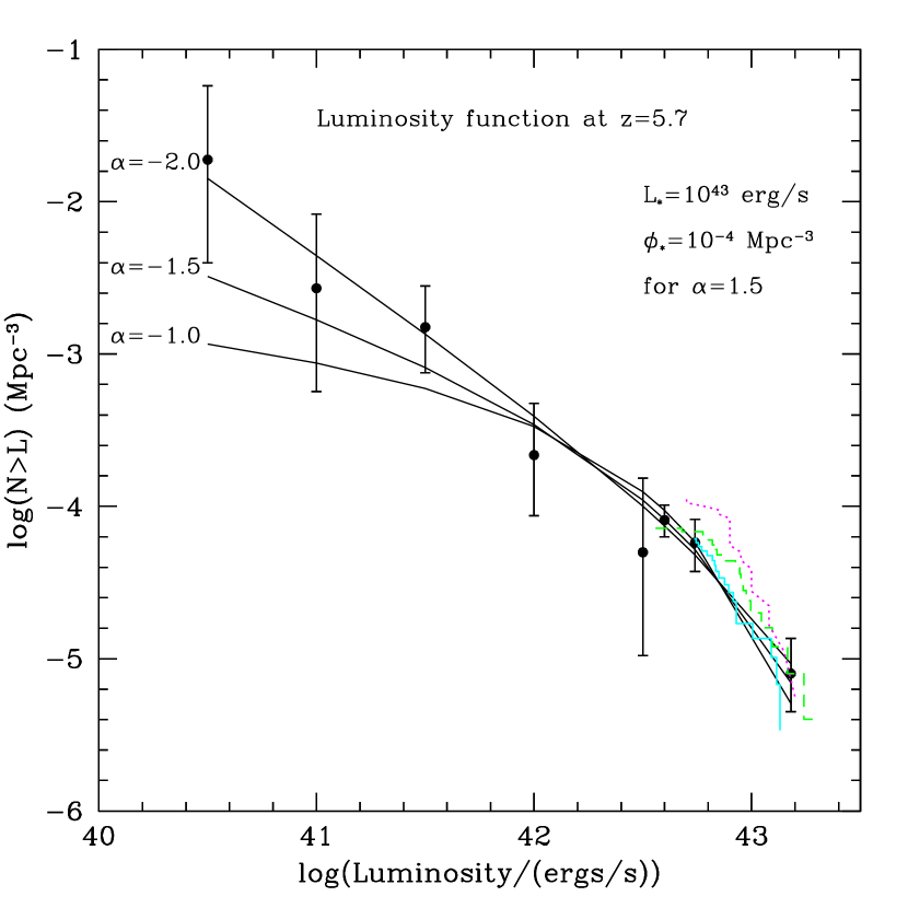
Figure 1: Lyman-$\alpha$ luminosity function at redshift $z\approx 5.7$. Data points with error bars show the measured densities above detection threshold and their corresponding uncertainties for samples from Table 1. Three curves are shown, corresponding to the best Schechter function fits to the data for assumed faint-end slopes $\alpha=1$, 1.5, and 2 (from bottom to top). Cumulative flux-number density curves are shown for the LALA survey (RM01 and Rhoads et al. 2003) - solid line , Hu et al. 2004 (dashed line), and Ajiki et al. 2003 - dotted line, and show consistency with each other.

3 The $z=6.5$ Lyman-$\alpha$ Luminosity Function

While the current sample of $z\approx 6.5$ Lyman-$\alpha$ emitters is small ($\sim 6$), they were identified by searches that spanned a wide range of survey volume (a factor of $\sim 10^{4}$) and sensitivity (a factor of $\sim 100$). The resulting sample can thus constrain the luminosity function reasonably. Table 2 lists the parameters of the various $z\gtrsim 6$ Lyman-$\alpha$ surveys that we consider in our analysis.

The LALA survey (Rhoads et al. 2000, 2003) covers the largest area, 1260 square arcminutes, to a depth of $2\times 10^{-17}{\rm\,erg\,cm^{-2}\,s^{-1}}$ at $z\approx 6.5$. Followup spectroscopy of three good candidates showed that one is a galaxy at $z=6.535$ and the other two are not (Rhoads et al 2004, hereafter R04). Kodaira et al. (2003; hereafter K03) use Subaru to search an area of 814 square-arcminutes to a depth of $0.9\times 10^{-17}{\rm\,erg\,cm^{-2}\,s^{-1}}$ and find 73 candidates. They obtained spectra for 9 of their candidates, among which two are confirmed as Lyman-$\alpha$ on the basis of a single asymmetric emission accompanied by a continuum drop, which would imply 16 Lyman-$\alpha$ sources among 73 candidates. Two further sources from K03 show asymmetric lines with a continuum too faint to ascertain a Lyman break. These are likely to also be Lyman-$\alpha$, resulting in a best estimate of 32 Lyman-$\alpha$ sources among the K03 candidates. The Hu et al. (2002) narrowband search for lensed sources finds intrinsically the faintest $z>6$ Lyman-$\alpha$ object after applying the factor of 4.5 lensing magnification in the smallest area, $0.46\Box^{\prime}$ with limiting line flux $3\times 10^{-18}{\rm\,erg\,cm^{-2}\,s^{-1}}$. Their larger area non-lensed upper limits are consistent with other surveys. The Santos et al (2004) spectroscopic survey for lensed Lyman-$\alpha$ emitters provides the deepest Lyman-$\alpha$ emitter search at $z\approx 6.5$ also. However, at $z>5.6$, Santos et al found no sources and thus provide only upper limits to the luminosity function. Kurk et al (2004) have reported the detection of one $z\approx 6.5$ source in a slitless spectroscopic search at the VLT. Their volume coverage is about 10% those of K03 and of R04, and their sensitivity ranges from $1$ to $2\times 10^{-17}{\rm\,erg\,cm^{-2}\,s^{-1}}$ depending on the line wavelength.

Cuby et al. (2003) report one source at z=6.17 found as a continuum drop source using narrow-band data. We neglect this source in the subsequent analysis because of the dissimilarity in discovery methods. Also, Stern et al (2004) have recently discovered a serendipitous $z\approx 6.5$ Lyman-$\alpha$ source in slit spectroscopy for an unrelated project. We leave this source also out of the present paper both because we came to know of it after most of our analysis was complete and because it is difficult to assess the true total volume in which serendipitous $z\approx 6.5$ galaxies might have been found and reported by extragalactic astronomers worldwide.

The density of Lyman-$\alpha$ emitters and its effective uncertainty is easily calculated for the LALA survey, Hu et al 2004, and Kurk et al 2004, all of which have complete spectroscopic followup of a small number of candidates. For the K03 sample, we need to account for spectroscopic completeness in two ways. First, K03 did not consider a source confirmed as Lyman-$\alpha$ unless it showed both line asymmetry and a continuum break. This, in our opinion, is too stringent, given that more than half of our $z=4.5$ sources remain undetected in the continuum due to high equivalent width of the Lyman-$\alpha$ line (Malhotra & Rhoads 2002) and still show the continuum break in coadded spectra (Dawson et al. 2004). Such a selection also biases against high equivalent width objects. Therefore we include all four of the Kodaira sources discussed above as Lyman-$\alpha$ in our luminosity function calculations. However our primary conclusions do not change qualitatively if we treat only two K03 objects as confirmed.

Second, the uncertainty in the K03 density estimate is dominated by the small size of the spectroscopic followup. Applying the same method we used for the $z\approx 5.7$ LALA and Hu et al samples, we find a variance of $20/9$ and fractional uncertainty of $37\%$ for the confirmed sample size. Adding in the small Poisson uncertainty in the candidate counts gives a fractional uncertainty of $39\%$ in the true Lyman-$\alpha$ source density. The equivalent number of objects for a pure Poisson sample would be $N_{equiv}=6.57$. Thus, we treat K03 as having discovered 6.57 sources in an effective volume $20\%=6.57/(73*4/9)$ of their true survey volume for purposes of our fitting code.

Table 2: Surveys at $z\approx 6.5$

Survey ID	Sensitivity	Volume	Number	$\sigma$
	(${\rm\,erg\,cm^{-2}\,s^{-1}}$)	(Mpc-3)
LALA (Rhoads et al. 2004)	$2\times 10^{-17}$	$2.11\times 10^{5}$	1	1
Kurk et al. 2004	$1.5\times 10^{-17}$	$1.8\times 10^{4}$	1	1
Kodaira et al 2003	$9\times 10^{-18}$	$2.2\times 10^{5}$	32.4	12.6
Hu et al. 2002	$3\times 10^{-18}$	110	1	1
Santos et al. 2004	$2.5\times 10^{-16}$	$2.7\times 10^{4}$	0
	$8\times 10^{-17}$	18929	0
	$2.5\times 10^{-17}$	11943	0
	$8\times 10^{-18}$	3000	0
	$2.5\times 10^{-18}$	598	0
	$8\times 10^{-19}$	78.9	0
	$2.5\times 10^{-19}$	11.4	0

Note. — Surveys used for determining the $z\approx 6.5$ Lyman-$\alpha$ luminosity function.

We then minimize the Cash parameter for the $z\approx 6.5$ data. These results are given in table 3, and plotted in figure 2. The Hu et al. (2003) lensed object HCM 6A, is incosistent with Santos et al. upper limits. If the surface density suggested by the HCM 6a discovery were the norm, Santos et al. (2004) should have detected 7 Lyman-$\alpha$ emitters at $5.6\lesssim z\lesssim 6.7$. They found none. The corresponding Poisson likelihood is $9\times 10^{-4}$. Taking now our best fit curve, the chance that Hu et al would have found HCM 6a is $6.5\%$. Likely explanations for this inconsistency include (a) luck, or (b) systematic difficulties in estimating sensitivity thresholds and volumes, which depend critically on the details of cluster lens modelling for both Hu et al and Santos et al. If the true lensing amplification for HCM 6a were $\sim 1$ (and not $\sim 4.5$ as Hu et al suggest), its intrinsic flux would be $\sim 2\times 10^{-17}{\rm\,erg\,cm^{-2}\,s^{-1}}$. The volume covered by Hu et al’s survey to that depth is roughly 400 times the volume stated for an amplification $>4.5$. This would move HCM 6A to a brightness and number density comparable to the LALA and Kurk et al 2004 points.

Figure 2: Lyman-$\alpha$ luminosity function at redshift $z\approx 6.5$. Data points with error bars show the measured densities above detection threshold and their corresponding uncertainties for samples from Table 2. Three curves are shown, corresponding to the best Schechter function fits to the data for assumed faint-end slopes $\alpha=1$, 1.5, and 2 (from bottom to top). The $z=5.7$ best fit luminosity function is also consistent with the data (short dashed curve), but $z=5.7$ luminosity function with flux attenuation of a factor of three (long dashed curve) is ruled out (see details in section 4).

Table 3: Fitted luminosity function parameters

Redshift	$\alpha$	log$({L_{\star}}/{\rm\,erg\,s^{-1}})$	log${({\phi_{\star}}/\hbox{Mpc}^{-3})}$
5.7	-1	-3.6	43.45
	-1.5	-4.0	43.0
	-2	-4.8	42.75
6.5	-1	-2.9	42.5
	-1.5	-3.0	42.6
	-2	-3.3	42.7

Note. — Best fit Lyman-$\alpha$ luminosity function parameters, as a function of redshift and faint-end luminosity function slope $\alpha$.

4 Testing for Reionization

To test whether Lyman-$\alpha$ emission lines from $z\approx 6.5$ galaxies are attenuated by the scattering effects of a neutral intergalactic medium, we compare the observations at $z\approx 6.5$ to two hypothetical Lyman-$\alpha$ luminosity functions. In hypothesis (A), we use the best-fitting $z\approx 5.7$ Lyman-$\alpha$ luminosity function directly. This corresponds to the null hypothesis that the $z\approx 6.5$ IGM neutral fraction, $x_{n}(z\approx 6.5)$, is not substantially greater than $x_{n}(z\approx 5.7)$, and that there has been no strong evolution of the Lyman-$\alpha$ luminosity function. (Given that the intervening time is only $\approx 160\hbox{Myr}$, or about 17% the age of the universe, evolution is likely to be relatively modest.). These results are tabulated in Table 4.

With the $z=5.7$ luminosity function, LALA should have found 3.6 sources, but found one; Kurk et al. should have found 0.5 sources and found one, K03 survey should find about 14 sources and the estimate there is 16–32, depending on whether 2 or 4 of their published spectra are believed to be Lyman-$\alpha$ emitters. We see that the expected numbers in all surveys are within a factor of 2–3 of the observed values. Poisson noise aside, we know that variation in number density of factors of 2–3 are often seen and are due to large scale structure. Therefore we conclude that the z=6.5 discoveries are consistent with the z=5.7 luminosity function.

In model (B), we assume that the Lyman-$\alpha$ fluxes are reduced by a factor of $\sqrt{(}10)$, which corresponds roughly to the minimum reduction expected in a neutral IGM for any model considered by Santos (2004). For many plausible models, the reduction would be considerably larger, especially for low-luminosity sources which cannot carve a significant ionized bubble in the surrounding IGM. Again the results are tabulated in Table 4. With this luminosity function, LALA and Kurk et al. had 10% and 3% chances of finding a source in their survey, but lucky coincidences do happen.

Here, the K03 sample is the most constraining due to its large size. Under model (B) they should have only 1–2 real Lyman-$\alpha$ emitters. They have published spectroscopic followup of 9 out of 73 candidates and 2 to 4 are already specctroscopically confirmed as Lyman-$\alpha$ emitters. We calculate the likelihood of obtaining the observed spectroscopic confirmations by modelling the number of Lyman-$\alpha$ emitters in the field with a Poisson random variable, and the number of spectroscopic confirmations achieved with a binomial probability distribution. This gives a likelihood of $6\%$ for $\geq 4$ spectroscopic confirmations under hypothesis (A) (and $40\%$ for $\geq 2$ confirmations). Adopting instead hypothesis (B) reduces the likelihood to $8\times 10^{-5}$ for $\geq 4$ confirmations (and $1.1\%$ for $\geq 2$ confirmations). Thus imposing a $3\times$ reduction in Lyman-$\alpha$ line fluxes reduces the likelihood for the K03 data by a factor of $\gtrsim 40$. The Hu et al. galaxy HCM 6A is unlikely to have been discovered, with 2% and 0.5% probability under the two luminosity function models, and does not fit with a best-fit luminosity function for z=6. See section 3 for further discussion.

Table 4: Comparison of $z\approx 6.5$ data to model luminosity functions

	LALA	Kurk	Kodaira	Hu
Observed	1	1	32.4	1
$z=5.7$ (raw)	3.6	0.55	14.3	0.02
$z=5.7$ (0.5 dex attenuated)	0.10	0.029	1.7	0.005

Note. — Comparison between observed and modelled Lyman-$\alpha$ galaxy sample sizes. The observed number is the candidate count corrected for spectroscopically determined reliability where appropriate. The “z=5.7 (raw)” line shows the expected number of Lyman-$\alpha$ emitters in each survey assuming that the best fitting $z\approx 5.7$ LF holds for $z\approx 6.5$. The “attenuated” line corresponds to the $z\approx 5.7$ LF with $L_{\star}$ reduced by a factor of $\sqrt{10}$ (and $\phi_{\star}$ unchanged). This approximates the effect of a neutral IGM on the observed Lyman-$\alpha$ lines under conservative assumptions.

5 Star Formation and Metal Production

We now estimate the star formation rate density in Lyman-$\alpha$ galaxies at $z\approx 5.7$ and $z\approx 6.5$ by integrating over a Schechter luminosity function. The luminosity density in Lyman-$\alpha$ photons is $L_{\star}\phi_{\star}(\alpha+1)!$ (e.g., Peebles 1993). At $z\approx 5.7$ and $\alpha=-1.5$, we obtain a luminosity density of ${\cal L}_{Ly\alpha}(5.7)=1.8\times 10^{39}{\rm\,erg\,s^{-1}}\hbox{Mpc}^{-3}$, corresponding to an SFRD of $1.8\times 10^{-3}M_{\odot}\hbox{yr}^{-1}\hbox{Mpc}^{-3}$. At $z\approx 6.5$ and $\alpha=-1.5$, the best fitting luminosity function implies a luminosity density of ${\cal L}_{Ly\alpha}(6.5)=7\times 10^{39}{\rm\,erg\,s^{-1}}\hbox{Mpc}^{-3}$, corresponding to an SFRD of $7\times 10^{-3}M_{\odot}\hbox{yr}^{-1}\hbox{Mpc}^{-3}$. As discussed in section 4, the $z\approx 6.5$ data are consistent with the $z\approx 5.7$ LF, which means that the differences in luminosity and SFR densities are within the measurement uncertainties. We therefore adopt $\sim 3\times 10^{-3}M_{\odot}\hbox{yr}^{-1}\hbox{Mpc}^{-3}$ as a weighted average estimate for Lyman-$\alpha$ galaxies at $z\sim 6$. Uncertainties in the luminosity functions lead to a factor of $\sim 3$ uncertainty in this SFRD.

This result substantially exceeds the lower bounds obtained from the input surveys without integrating over a luminosity function. For example, K03 find $5.2\times 10^{-4}M_{\odot}\hbox{yr}^{-1}\hbox{Mpc}^{-3}$, about 1/5 of our value. A lower bound from the Lyman break galaxies is $\geq 4.7\times 10^{-4}M_{\odot}\hbox{yr}^{-1}\hbox{Mpc}^{-3}$ at $5.6<z<6.1$ (Stanway, Bunker, & McMahon 2003), consistent with the K03 lower bound and again below the Lyman-$\alpha$ luminosity function integral. The omission of galaxies with active star formation but no prominent Lyman-$\alpha$ line (e.g. Malhotra et al. 2004) from the samples we consider can only increase the $z\approx 6.5$ SFRD above our estimate. Of course, the stellar population model used to derive the conversion between Lyman-$\alpha$ photons and star formation activity is sensitive to unknown details of the IMF and metallicity evolution at high redshift, and may be incorrect. Comparison with other methods of estimating the SFRD may be sensitive to these assumptions.

The metal production rate from the Lyman-$\alpha$ galaxies at $z\sim 6$ can be estimated because both Lyman-$\alpha$ photons and heavy elements are produced predominantly by the most massive stars. We use the relation $dM_{Z}/dt=500L_{i}/c^{2}$, where $L_{i}\gtrsim 2L_{Ly\alpha}$ is the luminosity in ionizing photons and $M_{Z}$ is the mass in elements with atomic number $Z\geq 6$ (Madau & Shull 1996). This gives a metal production rate of of $53M_{\odot}/\hbox{Myr}/\hbox{Mpc}^{3}\times{{\cal L}_{Ly\alpha}}/(3\times 10^{39}{\rm\,erg\,s^{-1}}\hbox{Mpc}^{-3})$. For comparison, the UV luminosity density in continuum-selected objects at $z\sim 4$ (uncorrected for dust absorption) implies a metal production of $85M_{\odot}/\hbox{Myr}/\hbox{Mpc}^{3}$ (Madau & Shull 1996).

Multiplying our metal production rate by the $0.85\hbox{Gyr}$ age of the universe at $z\approx 6.5$ gives an estimate of $4.5\times 10^{4}M_{\odot}/\hbox{Mpc}^{3}$ for the mean volume density of metals, or a mean metallicity estimate of $7\times 10^{-6}$ (for $\Omega_{b,0}=0.048$). This is about $7\%$ of the metal production required to reionize the universe with UV photons produced by stellar nucleosynthesis (Gnedin & Ostriker 1996).

6 Discussion and Conclusions

We show that the Lyman-$\alpha$ galaxy population at $z\approx 6.5$ shows no evidence for a neutral intergalactic medium, by comparing the $z\approx 6.5$ Lyman-$\alpha$ survey results to a Lyman-$\alpha$ luminosity function derived at $z\approx 5.7$. The $z\approx 6.5$ data are fitted by the $z\approx 5.7$ luminosity function with an acceptable likelihood, but the alternative hypothesis that all Lyman-$\alpha$ fluxes are attenuated by a factor of $\sim 3$ is much less likely. All but one data points, taken in different parts of the sky, are consistent with the luminosity function at that redshift bin, therefore we do not see any evidence of patchy reionization, which would attenuate Lyman-$\alpha$ in one patch and not the other. Within the limitation of small number of fields considered here, we do not see any evidence of ”reionization in progress”. More data would, of course, help.

We also derive the best fitting Schechter function parameters for both the $z\approx 5.7$ and $z\approx 6.5$ samples, and use the results to estimate the star formation rate density ($\sim 3\times 10^{-3}M_{\odot}\hbox{yr}^{-1}\hbox{Mpc}^{-3}$) and metal production ($\sim 50M_{\odot}\hbox{Myr}^{-1}\hbox{Mpc}^{-3}$) in Lyman-$\alpha$ galaxies at $z\sim 6$. These rates imply that Lyman-$\alpha$ emitters contribute $\sim 7\times 10^{-6}$ to the mean metallicity of the universe by redshift $6.5$, and contribute $\sim 7\%$ of the ultraviolet photon budget needed to reionize the universe.

The Lyman-$\alpha$ test it is sensitive to neutral fractions $x_{n}$ in the range $0.1\lesssim x_{n}\lesssim 1$. It therefore complements the Gunn-Peterson test, which “saturates” for very small IGM neutral fractions ($x_{n}\sim 10^{-4}$ in a uniform IGM, and $x_{n}\lesssim 10^{-2}$ in any case; e.g., Fan et al 2002). Our present result implies $x_{n}\ll 1$ (and probably $x_{n}\lesssim 0.3)$ at $z\approx 6.5$. This represents the strongest upper limit presently available on the neutral fraction at this redshift. The WMAP result (Spergel et al 2003) provides an integral constraint on the ionized column density along the line of sight, but does not place so strong a constraint on any particular redshift. By combining all of these constraints, and other tests in future, it will be possible to build a much more complete observational history of reionization.

References

- (1) Ajiki,M et al. 2004, to appear in PASJ, astro-ph/0405222
- (2) Ajiki,M et al., 2003, AJ 126, 2091
- (3) Becker, R. H., et al. (SDSS consortium), 2001, AJ 122, 2850
- (4) Cash, W. 1979, ApJ, 228, 939
- (5) Cen, R. 2003, ApJ, 591, 12.
- (6) Cuby, J.-G., LeFevre, O., McCracken, H., Cuillandre, J.-C., Magnier, E., & Meneux, B. 2003, A&A 405, L19
- (7) Dawson, S., Rhoads, J., Malhotra, S., Stern, D., Dey, A., Jannuzi, B, Wang, J.X., Landes, E. et al 2004, submitted to the ApJ.
- (8) Djorgovski, S. G., Castro, S. M., Stern, D., & Mahabal, A. 2001, ApJ, 560, L5.
- (9) Fan, X., Narayanan, V. K., Strauss, M. A., White, R. L., Becker, R. H., Pentericci, L., & Rix, H.-W. 2002, AJ 123, 1247
- (10) Gnedin, N., Ostriker, J.P. 1997 ApJ,486,581
- (11) Haiman, Z., & Spaans, M. 1999, ApJ 518, 138
- (12) Haiman, Z. 2002, ApJ 576, L1
- (13) Holder, G. Haiman, Z., & Mohr, J. J. 2001, ApJ 560, L111
- (14) Hu, E. M., Cowie, L. L., McMahon, R. G., Capak, P., Iwamuro, F., Kneib, J.-P., Maihara, T., Motohara, K. 2002, ApJ 568, L75
- (15) Hu, E. M., Cowie, L. L., , Capak, P., McMahon, r. g., Hayashino, T., & Komiyama, Y. 2004, AJ, 127,563.
- (16) Kodaira, K., et al 2003, PASJ 55, L17 (K03)
- (17) Kurk, J. D., Cimatti, A., di Serego Alighieri, S., Vernet, J., Daddi, E., Ferrara, A., & Ciardi, B. 2004, submitted to A&A, astro-ph/0406140
- (18) Loeb, A. & Rybicki, G. B. 1999, ApJ 524, L527
- (19) Madau, P., & Shull, J. M. 1996, ApJ 457, 551
- (20) Malhotra, S., & Rhoads, J. E. 2002, ApJ 565, L71
- (21) Malhotra, S., Rhoads, J., Pirzkal, N., Xu, C. et al. 2004 (in prep).
- (22) Martin, C. L., & Sawicki, M. 2004, ApJ 603, 414
- (23) Miralda-Escudé, J. 1998, ApJ 501, 15
- (24) Peebles, P. J. E., 1993, Principles of Physical Cosmology, Princeton: Princeton University Press
- (25) Pello, R., Schaerer, D., Richard, J., Le Borgne, J-F, Kneib, J-P 2004, astro-ph/0403025.
- (26) Pentericci, L. Fan, X., Rix, H.W., et al 2002, AJ,123, 2151
- (27) Rhoads, J. E., Malhotra, S., Dey, A., Stern, D., Spinrad, H., & Jannuzi, B. T. 2000, ApJ 545, L85
- (28) Rhoads, J. E., & Malhotra, S. 2001, (RM01) ApJ 563, L5
- (29) Rhoads, J. E., Dey, A., Malhotra, S., Stern, D., Spinrad, H., Jannuzi, B. T., Dawson, S., Brown, M. J. I., & Landes, E. 2003, AJ 125, 1006
- (30) Rhoads, J.E., Xu, C., et al. 2004, to appear in ApJ (astro-ph/0403161)
- (31) Santos, M. R. 2004, MNRAS, 349, 1137
- (32) Santos, M. R., Ellis, R. S., Kneib, J.-P., Richard, J., & Kuijken, K. 2004, ApJ, 606, 683
- (33) Spergel, D. N., et al 2003, ApJS, 148, 175
- (34) Stanway, E., Bunker, A., & McMahon, R. G. 2003, MNRAS 342, 439
- (35) Stern, D., et al 2004, submitted, astro-ph 0407409