Auto and cross correlation of phases of the whole-sky CMB and foreground maps from the 1-year WMAP data

Abstract

The issue of non-Gaussianity is not only related to distinguishing the theories of the origin of primordial fluctuations, but also crucial for the determination of cosmological parameters in the framework of inflation paradigm. We present a method for testing non-Gaussianity on the whole-sky CMB anisotropies. This method is based on the Kuiper’s statistic to probe the two-dimensional uniformity on a periodic mapping square associating phases: return mapping of phases of the derived CMB (similar to auto correlation) and cross correlations between phases of the derived CMB and foregrounds. Since phases reflect morphology, detection of cross correlation of phases signifies the contamination of foreground signals in the derived CMB map. The advantage of this method is that one can cross check the auto and cross correlation of phases of the derived maps and foregrounds, and mark off those multipoles in which the non-Gaussianity results from the foreground contaminations. We apply this statistic on the derived signals from the 1-year WMAP data. The auto-correlations of phases from the ILC map shows the significance above 95% CL against the random phase hypothesis on 17 spherical harmonic multipoles, among which some have pronounced cross correlations with the foreground maps. We find that most of the non-Gaussianity found in the derived maps are from foreground contaminations. With this method we are better equipped to approach the issue of non-Gaussianity of primordial origin for the upcoming Planck mission.

1 Introduction

The issue of non-Gaussianity in the cosmic microwave background (CMB) has touched the most fundamental base in cosmology. It was first brought to attention by Ferreira, Magueijo and Górski [Ferreira, Magueijo & Górski 1998] that non-Gaussian signal is present in the COBE data. Although it is almost certain that the departure from Gaussianity is induced by systematic error [Banday, Zaroubi & Gorski 2000, Magueijo & Medeiros 2004], the discussions and focus about non-Gaussianity since then have been focusing primarily on primordial origin. Mechanisms other than the simplest inflation model that have been proposed for primordial density fluctuations produce non-Gaussian fields (see Bartolo et al. 2004 and references therein). Due to this reason, the issue of non-Gaussianity seems to be discussed separately from that of the determination of cosmological parameters. It is in the framework of inflation paradigm that the cosmological parameters can only be determined correctly from the angular power spectrum if the CMB temperature anisotropies constitute a Gaussian random field (GRF). Therefore, the issue of non-Gaussianity is not beyond the power spectrum, but still within the power spectrum.

The statistical characterization of temperature fluctuations of CMB radiation on a sphere can be expressed as a sum over spherical harmonics:

$$\Delta T(\theta,\varphi)=\sum_{\ell=1}^{\infty}\sum_{m=-\ell}^{\ell}a_{\ell m}Y_{\ell m}(\theta,\varphi),$$ (1)

where $a_{\ell m}=|a_{\ell m}|\exp(i\phi_{{{\ell}m}})$. The strict definition of a homogeneous and isotropic GRF, as a result of the inflation paradigm, requires that the moduli $|a_{\ell m}|$ are Rayleigh distributed and the phases $\phi_{{{\ell}m}}$ are uniformly random on the interval $[0,2\pi]$. The central limit theorem, however, guarantees that a superposition of a large number of harmonic modes will be close to a Gaussian as long as the phases are random. Hence the random-phase hypothesis on its own serves as a definition of Gaussianity [Bardeen et al. 1986, Bond & Efstathiou 1987].

One of the most useful properties of GRF is that the second-order statistics, the 2-point correlation function or the angular power spectrum $C_{\ell}$

$$\langle a_{\ell m}a^{*}_{\ell^{{}^{\prime}}m^{{}^{\prime}}}\rangle=C_{\ell}\;\delta_{\ell\ell^{{}^{\prime}}}\delta_{mm^{{}^{\prime}}}$$ (2)

furnish a complete description of the GRF. It is based on this analytically-simple but important property that the cosmological parameters can be correctly determined from $C_{\ell}$. Accordingly, if non-Gaussian signals are present, either with primordial origin, or induced from data processing or systematic error, the cosmological parameters derived from the $C_{\ell}$ of such a “contaminated” field will have larger error bars. The issue of non-Gaussianity in CMB is therefore not only related to discriminating the theories of origin of primordial fluctuations, it is also fundamental, in the framework of inflation paradigm, for the determination of the cosmological parameters.

To test non-Gaussianity, the next order statistics: the 3-point correlation function, or its Fourier transform, the bispectrum are often used. The higher-order statistics, however, are only part of the whole picture about non-Gaussianity. It takes a full hierarchy of $n$-point correlation functions, or the polyspectra, to complete the statistical characterisation of the CMB anisotropies.

Since the release of 1-year WMAP data, great efforts have been made for the search and detection of non-Gaussianity via various approaches and methods [Chiang et al. 2003, Park 2004, Eriksen et al. 2004c, Vielva et al. 2004, Copi, Huterer & Starkman 2004, Eriksen et al. 2004b, Cabella et al. 2004, Hansen et al. 2004, Mukherjee & Wang 2004, Larson & Wandelt 2004]. These detection of non-Gaussianity shall augment the error bars on the estimation in cosmological parameters.

Practically speaking, characterizing non-Gaussianity through phases is one of the most general approaches. Based on the random-phase hypothesis, the key to developing statistical methods using phases is testing their “randomness”. Due to the $2\pi$ wrapping, however, the phases tend to be uniformly distributed at $[0,2\pi]$. For example, for a point source produces phases are distributed evenly and orderly, but not randomly between 0 and $2\pi$. Probing non-Gaussianity via examining uniformity of phases themselves between 0 and $2\pi$ is often as ineffective as via examining one-point Gaussian (temperature) probability distribution $p(T)$ (e.g. it is possible $p(T)$ is still Gaussian for a non-Gaussian field). The $2\pi$ wrapping causing a uniform distribution of phases is similar to the central limit theorem in action producing one-point Gaussian probability distribution. We thus seek associations between phases as a more sensitive and effective statistical measure.

The linear association such as auto correlation $\langle\phi\phi^{{}^{\prime}}\rangle$, however, does not give useful statistics due to the circular nature of phases. To counter this problem, return mapping of phases is introduced to associate phase pairs systematically [Chiang, Coles & Naselsky 2002]. The main idea is mapping all phase pairs with the same separation $(\Delta{\ell},\Delta m)$ onto a square, which is conceptually similar to the auto correlation $\xi(\Delta{\ell},\Delta m)=\langle\phi_{{\ell},m}\,\,\phi_{{\ell}+\Delta{\ell},m+\Delta m}\rangle$.

Another important feature of phases is that phases are closely related to morphology. Through pixel-by-pixel cross correlation, maps with the same phases display strong resemblance in morphology, regardless of their power spectrum [Chiang 2001]. The level of cross-correlation of phases taken from two images therefore renders significance of resemblance between them. Based on the simple but prevailing assumption that the CMB signals should not correlate with the foregrounds (i.e. the microwave foregrounds should not have knowledge in what the CMB signals ‘look like’), cross correlations of phases between the derived CMB and the foregrounds shed light on the status of microwave foreground cleaning. Dineen and Coles [Dineen & Coles 2003] perform cross correlations in pixel domain between the derived CMB and the foreground maps. Naselsky, Doroshkevich & Verkhodanov [Naselsky, Doroshkevich & Verkhodanov 2003, Naselsky, Doroshkevich & Verkhodanov 2004], Naselsky et al.[Naselsky et al. 2004] use cross correlation of phases to illustrate the foreground contaminations in the derived CMB signals.

Return mapping of phases renders phase associations on a square with each side ranged $[0,2\pi]$ (with periodic boundaries). Cross correlation of phases between derived CMB and foregrounds connect phases from the same $a_{\ell m}$ mode of the maps also produce mapping in a $[0,2\pi]$ square. The null hypotheses for both cases: random phases for a Gaussian CMB sky and no cross correlation between the CMB and the foregrounds shall result in random points on $[0,2\pi]$ squares. Statistics that are developed for a square taking into account of the periodic boundaries can be implemented both on the return mapping (auto correlation of phases) of the derived CMB signal and on cross correlation of phases between CMB and foregrounds. More importantly, through checking both auto and cross correlations of phases from the derived maps, one can gain insight into the issue of non-Gaussianity.

In this paper we test on each spherical harmonic multipole ${\ell}$ the auto and cross correlations, as well as the overall correlations. This paper is arranged as follows. In Section 2 we recap the phase mapping technique and introduce the Kuiper’s statistics. We apply the Kuiper’s statistics in Section 3 both on the auto and cross correlation of phases of the 1-year WMAP derived maps and connect the phase correlations with non-trivial whitened $\Delta T$ distribution in 1D Fourier composition. The conclusion and discussions are in Section 4.

2 The phase mapping technique and the Kuiper’s statistics

2.1 The return mapping of phases and two-dimensional uniformity

Chiang, Coles & Naselsky [Chiang, Coles & Naselsky 2002] have introduced a technique called return mapping of phases to render associations between phase pairs on a square. The idea is borrowed from the return map in chaotic dynamics [May 1976]. The phase pairs are taken systematically and mapped onto a $[0,2\pi]$ square. In a return map of phase pairs with the separation $(\Delta{\ell},\Delta m)$, for example, the mapped points formed from phase pairs have the coordinates $(\phi_{{\ell},m}\,\,,\phi_{{\ell}+\Delta{\ell},m+\Delta m})$ for all possible ${\ell}$ and $m$. Because of the circular nature of phases, the $[0,2\pi]$ return map is periodic at all 4 sides, which can be viewed as a flat torus.

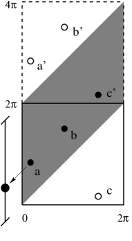
Figure 1: We show two panels formed with a mosaic of 4 return maps of phases (left) and the projection of the mapping points to tackle the circular nature of phases. On the left top, the 4 points $\beta$, $\gamma$, $\varepsilon$ and $\eta$ on the return maps in fact represent the same point due to periodicity of the return maps. To probe the connectivity of points on the return maps, therefore, we consider the simplest directions: anti-diagonal ($\vec{\rm BD}$), and diagonal ($\vec{\rm AC}$) projecting onto the $y$ axis. On the right panel, we put 3 points $a$, $b$ and $c$, as an example on the return map and probe the connectivity in the anti-diagonal direction. We reproduce the same map on top of it: ${\mbox{\boldmath$a$}^{{}^{\prime}}}$, ${\mbox{\boldmath$b$}^{{}^{\prime}}}$ and ${\mbox{\boldmath$c$}^{{}^{\prime}}}$. Due to the projection, we consider the same total area but different configuration (the shaded area), which covers the 2 points from the lower map ($a$ and $b$), and 1 from the upper map (${\mbox{\boldmath$c$}^{{}^{\prime}}}$). The 3 seemingly non-correlated points in a single return map now show the alignment along the anti-diagonal direction.

After the mapping of phases, various statistics can be applied to extract the statistical significance. Chiang, Naselsky & Coles [Chiang, Naselsky & Coles 2004] use a simple mean chi-square statistic to extract the information of the one-dimensional uniformity of the distribution of the return maps. In order to probe associations between points (uniformity in 2 dimensions), care has to be taken on the periodicity of the return maps. In Fig.1 on the left we show the mosaic of 4 return maps to indicate the periodicity. To probe the connectivity of points on the return maps, we consider the following 2 directions: anti-diagonal ($\vec{\rm BD}$), and diagonal ($\vec{\rm AC}$) onto the $y$ axis. This projection is also useful for cross correlation of phases. Complete cross correlation of phases produces points exactly on the anti-diagonal line.

The projection of a point located at $(x_{0},y_{0})$ along the anti-diagonal direction to $y$ axis as shown in Fig.1 is equivalent to taking the difference of its $x$ and $y$ coordinates, i.e. $y_{0}-x_{0}$; in the diagonal direction $y_{0}+x_{0}$. In a return map of phases with separation $(\Delta{\ell},\Delta m)$, points are formed with phase pairs $\phi_{{\ell}m}$ and $\phi_{{\ell}+\Delta{\ell},m+\Delta m}$, the projection then becomes $\phi_{{\ell}+\Delta{\ell},m+\Delta m}-\phi_{{\ell}m}$: the phase difference. In Coles et al. [Coleset al. 2003] they probe phase correlations by investigating the uniformity of the neighbouring phase difference $\phi_{{\ell},m+1}-\phi_{{\ell}m}$. This is equivalent to testing the uniformity of the projected points on a return map of the separation $(\Delta{\ell},\Delta m)=(0,1)$. Following this line of thought, the analysis of the projection in either the vertical or the horizontal directions is that of the randomness of $\phi_{{\ell}m}$ themselves.

Figure 2: The difference in the statistical significance of Kuiper statistics from its analytical derivation, Eq.(5) and (6), and Monte Carlo simulation. We list the 3 frequently used significance value (from top to bottom): 66.269%, 95.450% and 99.730%, respectively, which corresponds to Gaussian 1, 2, 3-$\sigma$ C.L.. The $y$-axis is the difference in absolute value, and the $x$-axis is the data point $N$.

2.2 The Kuiper’s statistic

The Kuiper’s statistic can be viewed as a variant of Kolmogorov-Smirnov (K-S) test [Kuiper 1960, Press et al. 1992, Fisher 1993]. As the projection of points on the directions we mention in § 2.1 produces unbinned distribution that is a function of single independent variable, it is very useful to apply the K-S test to probe its uniformity. The K-S statistic is taken as the maximum distance of the cumulative proability distribution against the theoretical one:

$$D=\max_{-\infty<x<\infty}|S_{N}(x)-P(x)|$$ (3)

For circular function, however, one needs to take into account of the maximum distance both above and below the $P(x)$

$$V=D_{+}+D_{-} = \max_{-\infty<x<\infty}[S_{N}(x)-P(x)]$$ (4)

$$+ \max_{-\infty<x<\infty}[P(x)-S_{N}(x)]$$

and the C.L. against the null hypothesis (e.g. uniformity of phases in our case) can be calculated from [Press et al. 1992]

$${\rm C.L.}=1-Q_{\rm Kuiper}\left(V\left[\sqrt{N}+0.155+\frac{0.24}{\sqrt{N}}\right]\right),$$ (5)

where

$$Q_{\rm Kuiper}(\lambda)=2\sum^{\infty}_{j=1}(4j^{2}\lambda^{2}-1)e^{-2j^{2}\lambda^{2}},$$ (6)

and $N$ is the data points.

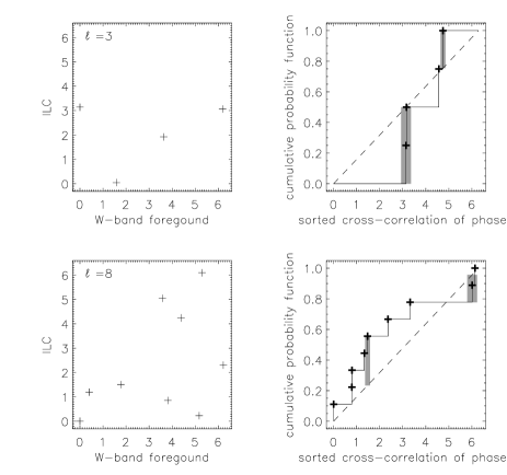
Figure 3: The cross correlation of phases at ${\ell}=3$ (top-left: $m=0-3$) and 8 (bottom-left: $m=0-8$) between the ILC map and the W-band foreground map. One can imagine that, for example, for ${\ell}=3$ the 4 points are highly correlated along the anti-diagonal direction if the left-most point is repositioned at the far-right. The same for ${\ell}=8$ if we reposition the 3 points at the lower-right region to the above top axis line (cf Fig.1). The panels on the right are their corresponding cumulative probability functions. The dashed line is the $P(x)$, the theoretical cumulative probability distribution for 2D uniformity. The thin and thick shaded lines are the $D_{+}$ and $D_{-}$, respectively, their maximum distances of the cumulative probability distribution above and below the theoretical one.

We run Monte Carlo (MC) simulation in order to test Eq.(5) and (6). One hundred thousand realizations of the difference of two random phase series (the phases are defined $[0,2\pi)$) are simulated, which is to mimic the projection of return map shown in Fig.1. For each $N$, we have an ensemble of 100 000 random realization each producing maximum distance $V$ as in Eq.(4). We then sort these 100 000 $V$ to yield the statistical significance from MC simulation. Simultaneously, the statistical significance can be calculated directly from Eq.(5) and (6). In Fig.2 we show the difference in the statistical significance of the Kuiper statistics from its analytical derivation, Eq.(5) and (6), and MC simulation. We list the 3 frequently quoted significance value (from top to bottom): 66.269%, 95.450% and 99.730%, which corresponds to Gaussian 1, 2, 3-$\sigma$ C.L., respectively. One can see that for 95.450% and 99.730% the difference between analytical calculation and MC simulation is down to $10^{-3}$ level even for as few data points as $N=10$.

We use the maps available on the WWW for testing this method: the derived foreground maps at 5 frequency bands from the WMAP website and the 4 derived CMB maps : the internal linear combination (ILC) map by the WMAP science team [Bennett et al. 2003a, Bennett et al. 2003b, Bennett et al. 2003c, Hinshaw et al. 2003a, Hinshaw et al. 2003b, Komatsu et al. 2003], the ILC map by Eriksen et al.(hereafter EILC) [Eriksen et al. 2004a] , the Wiener-filtered map (WFM) by Tegmark, de Oliveira-Costa & Hamilton [Tegmark, de Oliveira-Costa & Hamilton 2003], and the Phase-Cleaned Map (PCM) by Naselsky et al. [Naselsky et al. 2003]. Note that these maps are used only for testing the effectiveness of the Kuiper’s statistics because of their different approaches on foreground cleaning and their different morphology. Our claim about non-Gaussianity in this paper shall not contradict with others in the literature as most of these maps, as advised by the authors, are not for scientific purposes.

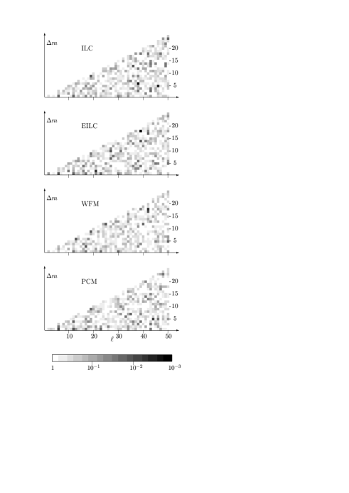
Figure 4: The Kuiper’s statistics on return maps for the WMAP ILC map, the EILC map, TOH’s Wiener-filter map and the PCM map. In order to display the C.L. more clearly against random phase hypothesis, we show the $Q_{\rm Kuiper}$ instead. So $10^{-3}$ corresponds to C.L. 99.9% against uniformity of phases, $10^{-2}$ corresponds to C.L. 99% …etc.. Within each multipole ${\ell}$ we take the phases of fixed separation $\Delta m$ and map them in a return map. We take $\Delta m=1$ up to $\Delta m={\ell}_{0}/2$ for multipole number ${\ell}_{0}$.

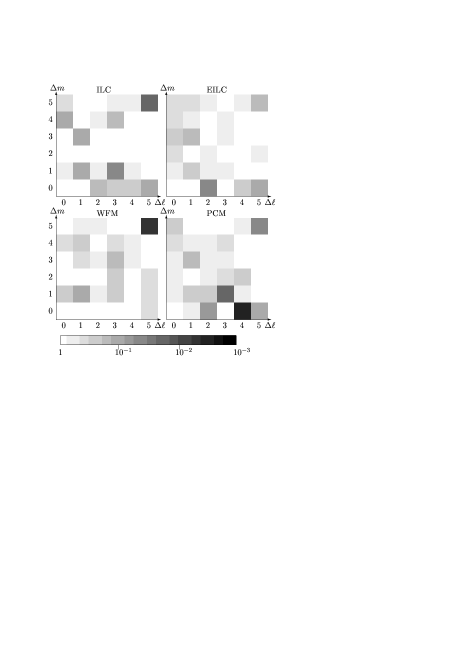
Figure 5: The Kuiper’s statistics on return map for separation $(\Delta{\ell},\Delta m)$. The mapping takes all the phases from ${\ell}=2$ to 50. The separation of mapping is ranged 0 to 5 for both $\delta{\ell}$ and $\delta m$. In order to display more clearly the C.L. against random phase hypothesis, we show the $Q_{\rm Kuiper}$ instead. So $10^{-3}$ corresponds to 99.9% C.L. against uniformity of phases, $10^{-2}$ to 99% C.L. …etc..

In Fig.3 as an example of how the Kuiper’s statistics works, we show the cross correlation of phases between the ILC and the W-band foreground map at ${\ell}=3$ (top) and ${\ell}=8$ (bottom) and their corresponding cumulative probability functions from the projection in the anti-diagonal direction onto the $y$ axis. We show with thin ($D_{+}$) and thick ($D_{-}$) shaded lines the maximum distances of the cumulative probability distribution above and below the theoretical one, respectively.

3 Auto and cross correlation of phases

3.1 Auto correlation

We consider first within each multipole number ${\ell}$ the mapping of phases of fixed $\Delta m$. In Fig.4 we show the Kuiper’s statistics on return maps for the WMAP ILC map, the EILC map, the WFM and the PCM. Within each multipole ${\ell}$ we take the phases of fixed separation $\Delta m$ and map them into a return map. For the multipole number ${\ell}={\ell}_{0}$ we take the separation from $\Delta m=1$ to $\Delta m={\ell}_{0}/2$, although in general we can take any $\Delta m$ values to test the randomness of phases. In order to display the C.L. more clearly against random phase hypothesis, we show the $Q_{\rm Kuiper}$ instead. So $10^{-3}$ corresponds to C.L. 99.9% against uniformity of phases, $10^{-2}$ corresponds to C.L. 99% …etc..

One interesting result is that for ${\ell}=6$ the mapping of $\Delta m=1-3$ for all 4 maps are all above 75% C.L.. and the multipole numbers which has $\Delta m$ mappings that are above 95.45% C.L. against random phase hypothesis are ${\ell}=6$, 12, 15, 17, 19, 30, $35-36$, $38-39$, 41, 43, $45-47$, $49-50$. For $\Delta m=6$ at ${\ell}=38$ and $\Delta m=5$ at ${\ell}=46$, both mappings reach above 99.73%. For other 3 maps, they all have modes that reach 95.45%. We do not, however, claim the overall non-Gaussianity of these maps.

We also consider the mapping for separation $(\Delta{\ell},\Delta m)$ from all the available phases from ${\ell}=2$ to 50 (except those of $m=0$ modes). In Fig.5 we show the Kuiper’s statistics for the 4 maps: the ILC, EILC, WFM and PCM. The separation of return mapping ranges from 0 to 5 for both $\Delta{\ell}$ ($x$ axis), $\Delta m$ $y$ axis), although it can be extended to higher number. The ILC, EILC and PCM have $(\Delta{\ell},\Delta m)=(2,0)$ correlation above 68.27% C.L. and there are considerable degrees of phase correlation at separation $(\Delta{\ell},0)$ for ILC, EILC and PCM, but except for WFM.

Note also the strong correlation of $(\Delta{\ell},\Delta m)=(4,0)$ for the PCM. This specific correlation is recently mentioned in Naselsky & Novikov [Naselsky & Novikov 2005], which is caused by the symmetric (w.r.t. Galactic centre) point-like peaks lying along the Galactic plane. The PCM is produced without further cleaning performed for ILC, EILC and WFM, hence the Galactic contamination is still present.

Figure 6: The assembled “whitened” distribution ${\ell}$ by ${\ell}$ from the WMAP ILC map. We assemble only the phase part $\exp(i\phi_{{{\ell}m}})$ of each harmonic number ${\ell}$ in Fourier composition: $\Delta T_{{\ell},{\rm whitened}}(x)=\sum_{m}\exp(i\phi_{{{\ell}m}})\exp(imx)$. The extrema that reach $3\sigma$ are ${\ell}=6$, 12, 15 and 17: $-3.0\sigma$, $3.1\sigma$, $-3.2\sigma$ and $3.3\sigma$, respectively. These multiple numbers are picked up by phase correlations with C.L. 95.45% from the Kuiper’s statistics.

In order to see how non-random phases affect the distribution, we assemble only the phase part in each harmonic number ${\ell}$ in Fourier composition (the so-called “whitened” image):

$$\Delta T_{{\ell},{\rm whitened}}(x) \equiv \sum_{m}\frac{a_{\ell m}}{|a_{\ell m}|}\exp(imx)$$ (7)

$$= \sum_{m}\exp(i\phi_{{{\ell}m}})\exp(imx).$$

In Fig.6 we display for ${\ell}=2$ to 17 the “whitened” distributions which have no influence from the amplitudes $|a_{\ell m}|$. This representation in 1D Fourier composition for each ${\ell}$, rather than in the standard whole-sky spherical harmonic composition, can provide some advantages for further analysis. The morphology can be seen more clearly in 1D Fourier composition than in spherical harmonic composition. Here we can relate phase correlation (in Fourier space) to the simple GRF peak statistics (in real space). The extrema (maximum or minimum) that have reached $3\sigma$ appear in the distribution of ${\ell}=6$, 12, 15 and 17: $-3.0\sigma$, $3.1\sigma$, $-3.2\sigma$ and $3.3\sigma$, respectively. These multipole numbers correspond to those picked up by the Kuiper’s statistics with non-random phases at 95.45% C.L.. Furthermore, phase correlation does not only manifest itself in the extrema. One can see, for example, for ${\ell}=10$ the assembled whitened $\Delta T$ has repeated peaks. The C.L. against random phase hypothesis at $\Delta m=2$ of ${\ell}=10$ reaches 94.13%.

3.2 Cross correlation

The Kuiper’s statistics can also be applied to cross correlation.

In Fig.7 we show the C.L. against the null hypothesis in cross-correlation of phases for ${\ell}=2$ to 50. The thick lines are the WMAP ILC cross the WMAP foreground maps at (from top to bottom) K, Ka, Q, V and W-band, the cross sign ($\times$), the diamond sign ($\diamond$), the plus sign ($+$) are the EILC by Eriksen et al.[Eriksen et al. 2004a], the PCM by Naselsky et al.[Naselsky et al. 2003] and the WFM by Tegmark et al.[Tegmark, de Oliveira-Costa & Hamilton 2003], respectively, cross the WMAP foreground maps. We would like to point out that the ILC are produced by less weights from the W-band map than V and Q. One can see that the ILC map has substantial cross correlation of phases for ${\ell}=3$ and 8 with WMAP all 5 channel foreground maps. High cross correlation with the foregrounds, however, does not necessarily imply the non-Gaussianity for that multipole number.

In Fig.8 we show the assembled $\Delta T$ distribution for ${\ell}=8$ from WMAP ILC map and WMAP W-channel foreground map. From the Kuiper’s statistics for cross correlation of phases, for ${\ell}=8$ the correlation reaches C.L. 89.98%, which reflects on their resemblance in morphology.

4 Conclusion and Discussions

In this paper we introduce the Kuiper’s statistic to probe the 2D uniformity for the phase mapping technique. The Kuiper’s statistics are useful to explore both auto correlation and cross correlation of phases. We use the 4 maps to test the effectiveness of this method: WMAP ILC, the ILC by Eriksen et al., the WFM by Tegmark et al.and the PCM by Naselsky et al.and found several multipole numbers with non-randomness of phases over 95.45%. The Kuiper’s statistics can also used to test on all the available phases.

Contrary to the $\Delta T$ representation for each ${\ell}$ from standard spherical harmonic composition, we use 1D Fourier composition to display the $\Delta T$. We use the “whitened” Fourier composition to display the connection between non-random phases and non-trivial morphology, and between cross-correlated phases of 2 maps and resemblance in their morphology.

The peculiarity of ${\ell}=3$ and 8 found by Copi et al.[Copi, Huterer & Starkman 2004] can be seen clearly in the cross correlation with the foregrounds at all 5 foreground maps, as shown in Fig.7, particularly with the W band foreground map. This is another advantage of using phases as cross checking for non-Gaussianity for the CMB signal. There is no other method so far that can cross check both the foreground maps and the derived CMB map when peculiarities are found. What is unclear though, is the non-random phases at ${\ell}=6$ appearing on all ILC, EILC WFM, and PCM (Fig.4), where the cross correlation with foregrounds is reasonably low.

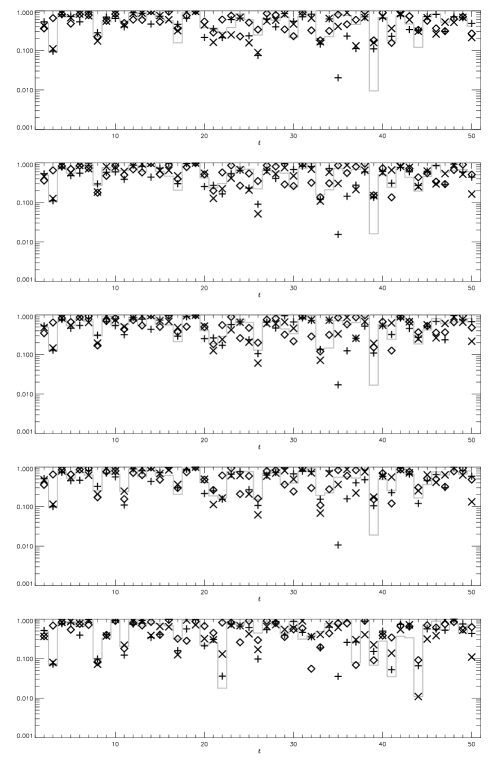
Figure 7: The confidence level against the null hypothesis in cross-correlation of phases for ${\ell}=2$ to 50. The thick lines are the WMAP ILC cross the WMAP foreground maps at (from top to bottom) K, Ka, Q, V and W-band, the cross sign ($\times$), the diamond sign ($\diamond$), the plus sign ($+$) are the EILC by Eriksen et al.[Eriksen et al. 2004a], the PCM by Naselsky et al.[Naselsky et al. 2003] and the WFM by Tegmark et al.[Tegmark, de Oliveira-Costa & Hamilton 2003], respectively, cross the WMAP foreground maps. In order to display the C.L. against random phase hypothesis more clearly, we show the $Q_{\rm Kuiper}$ instead. So 0.1 corresponds to 90% C.L. against uniformity of phases, 0.01 to 99% C.L. …etc..

Figure 8: The assembled $\Delta T$ distribution for ${\ell}=8$ from WMAP ILC map (solid curve) and WMAP W-channel foreground map (dashed curve). The top panel is assembled from $\sum_{m}a_{8m}\exp(imx)$ and the bottom (whitened) from $\sum_{m}\exp(i\phi_{8m})\exp(imx)$. Notice the resemblance in morphology between the derived CMB and foreground signals.

References

- [Banday, Zaroubi & Gorski 2000] Banday A. J., Zaroubi S., Gorski K. M., 2000, ApJ, 533, 575
- [Bardeen et al. 1986] Bardeen J. M., Bond J. R., Kaiser N., Szalay A. S., 1986, ApJ, 304, 15
- [Bartolo et al. 2004] Bartolo N., Komatsu E., Matarrese S., Riotto A., 2004, Phys. Rep. (astro-ph/0406398)
- [Bennett et al. 2003a] Bennett C. L. et al., 2003, ApJ, 583, 1
- [Bennett et al. 2003b] Bennett C. L. et al., 2003, ApJS, 148, 1
- [Bennett et al. 2003c] Bennett C. L. et al., 2003, ApJS, 148, 97
- [Bond & Efstathiou 1987] Bond J. R., Efstathiou G., 1987, MNRAS, 226, 655
- [Cabella et al. 2004] Cabella P., Hansen F., Marinucci D., Pagano D., Vittorio N., 2004, Phys. Rev. D, 69, 063007
- [Chiang 2001] Chiang L.-Y., 2001, MNRAS, 325, 405
- [Chiang 2003] Chiang L.-Y., 2004, MNRAS, 350, 1310
- [Chiang et al. 2002] Chiang L.-Y., Christensen P. R., Jørgensen H. E., Naselsky I. P., Naselsky P. D., Novikov D. I., Novikov I. D., 2002, A&A, 392, 369
- [Chiang & Coles 2000] Chiang L.-Y., Coles P., 2000, MNRAS, 311, 809
- [Chiang, Coles & Naselsky 2002] Chiang L.-Y., Coles P., Naselsky P. D., 2002, MNRAS, 337, 488
- [Chiang, Naselsky & Coles 2004] Chiang L.-Y., Naselsky P. D., Coles P., 2004, ApJL, 602, 1
- [Chiang et al. 2003] Chiang L.-Y., Naselsky P. D., Verkhodanov O. V., Way M. J., 2003, ApJ, 590, L65
- [Coles & Barrow 1987] Coles P., Barrow J. D., 1987, MNRAS, 228, 407
- [Coles & Chiang 2000] Coles P., Chiang L.-Y., 2000, nat, 406, 376
- [Coleset al. 2003] Coles P., Dineen P., Earl J., Wright D., 2004, MNRAS accepted (astro-ph/0310252)
- [Copi, Huterer & Starkman 2004] Copi C. J., Huterer D., Starkman G. D., 2004, Phys. Rev. D in press (astro-ph/0310511)
- [Dineen & Coles 2003] Dineen P., Coles P., 2003, MNRAS accepted (astro-ph/0306529)
- [Doroshkevich et al. 2003] Doroshkevich A. G., Naselsky P. D., Verkhodanov O. V., Novikov D. I., Turchaninov V. I., Novikov I. D., Christensen P. R., 2003, A&A submitted (astro-ph/0305537)
- [Eriksen et al. 2004a] Eriksen H. K., Banday A. J., Gorski K. M., Lilje P. B., 2004, ApJ, 612, 633
- [Eriksen et al. 2004b] Eriksen H. K., Hansen F. K., Banday A. J., Gorski K. M., Lilje P. B., 2004, ApJ, 605, 14
- [Eriksen et al. 2004c] Eriksen H. K., Novikov D. I., Lilje P. B., Banday A. J., Gorski K. M., 2004, ApJ, 612, 64
- [Ferreira, Magueijo & Górski 1998] Ferreira P., Magueijo J., Gorski K. M., 1998, ApJ, 503, L1
- [Fisher 1993] Fisher N. I., 1993, Statistical analysis of Circular Data, Cambridge University Press, Cambridge, UK
- [Gaztanagz & Wagg 2003] Gaztanagz E., Wagg J., 2003, Phys. Rev. D, 68, 021302
- [Górski, Hivon & Wandelt 1999] Górski K. M., Hivon E., Wandelt B. D., 1999, in A. J. Banday, R. S. Sheth and L. Da Costa, Proceedings of the MPA/ESO Cosmology Conference “Evolution of Large-Scale Structure”, PrintPartners Ipskamp, NL
- [Hansen et al. 2004] Hansen F. K., Cabella P., Marinucci D., Vittorio N., 2004, ApJL submitted (astro-ph/0402396)
- [Hikage, Matsubara & Suto 2003] Hikage C., Matsubara T., Suto Y., 2003, ApJ submitted (astro-ph/0308472)
- [Hinshaw et al. 2003a] Hinshaw G. et al., 2003, ApJS, 148, 63
- [Hinshaw et al. 2003b] Hinshaw G. et al., 2003, ApJS, 148, 135
- [Komatsu et al. 2003] Komatsu E. et al., 2003, ApJS, 148, 119
- [Kuiper 1960] Kuiper N. H., 1960, Proceedings of the Koninklijke Nederlandse Akademie van Wetenschappen, Series A, Vol 63
- [Larson & Wandelt 2004] Larson D. L., Wandelt B. D., 2004, ApJL submitted (astro-ph/0404037)
- [Magueijo & Medeiros 2004] Magueijo J., Medeiros J., 2004, MNRAS submitted (astro-ph/0311096)
- [Matsubara 2003] Matsubara T., 2003, ApJL, 591, 79
- [May 1976] May R. M., nat 261 459 1976
- [Mukherjee & Wang 2004] Mukherjee P., Wang Y., 2004, ApJ accepted (astro-ph/0402602)
- [Naselsky & Novikov 2005] Naselsky P. D., Novikov I. D., 2005, ApJL submitted (astro-ph/0503015)
- [Naselsky et al. 2003] Naselsky P. D., Verkhodanov O. V., Chiang L.-Y., Novikov I. D., 2003, ApJ submitted (astro-ph/0310235)
- [Naselsky et al. 2004] Naselsky P. D., Verkhodanov O. V., Chiang L.-Y., Novikov I. D., 2004, ApJ submitted (astro-ph/0405523)
- [Naselsky, Doroshkevich & Verkhodanov 2003] Naselsky P. D., Doroshkevich A., Verkhodanov O. V., 2003, ApJL 599 53 (astro-ph/0310542)
- [Naselsky, Doroshkevich & Verkhodanov 2004] Naselsky P. D., Doroshkevich A., Verkhodanov O. V., 2004, MNRAS 349 695 (astro-ph/0310601)
- [Cabella et al. 2004] Cabella P., Hansen F., Marinucci D., Pagano D., Vittorio N., 2004, Phys. Rev. D, 69, 063007
- [Park 2004] Park C.-G., 2004, MNRAS, 349, 313
- [Press et al. 1992] Press W. H., Teukolsky S. A., Vetterling W. T., Flannery B. P., 1992, Numerical Recipes in Fortran, Cambridge University Press, Cambridge, UK
- [Tegmark & Efstathiou 1996] Tegmark M., Efstathiou G., 1996, MNRAS, 281, 1297
- [Tegmark, de Oliveira-Costa & Hamilton 2003] Tegmark M., de Oliveira-Costa A., Hamilton A., 2003, Phys. Rev. D accepted (astro-ph/03022496)
- [Vielva et al. 2004] Vielva P., Martinez-Gonzalez E., Barreiro R. B., Sanz J. L., Cayon L., 2004, ApJ accepted (astro-ph/0310273)
- [Watts & Coles 2002] Watts P. I. R., Coles P., 2002, MNRAS, 338, 806
- [Watts, Coles & Melott 2003] Watts P. I. R., Coles P., Melott A., 2003, ApJL, 589, 61
- [Komatsu, Spergel & Wandelt 2003 ] Komatsu E., Spergel D. N., Wandelt B. D., 2004, ApJ (astro-ph/0305189)