Detailed spectral analysis of the 260 ksec XMM-Newton data of 1E1207.4-5209 and significance of a 2.1 keV absorption feature

Abstract

We have reanalyzed the 260 ksec XMM-Newton observation of 1E1207.4-5209. There are several significant improvements over previous work. Firstly, a much broader range of physically plausible spectral models was used. Secondly, we have utilized a more rigorous statistical analysis. The standard F-distribution was not employed, but rather the exact finite statistics F-distribution was determined by Monte-Carlo simulations. This approach was motivated by the recent work of Protassov et al. (2002) and Freeman et al. (1999). They demonstrated that the standard F-distribution is not even asymptotically correct when applied to assess the signficance of additional absorption features in a spectrum. With our improved analysis we do not find a third and fourth spectral feature (Bignami et al. (2003), De Luca et al. (2004)) in 1E1207.4-5209, but only the two broad absorption features previously reported (Sanwal et al. (2002), Hailey and Mori (2002)). Two additional statistical tests, one line model dependent and the other line model independent confirmed our modified F-test analysis. For all physically plausible continuum models where the weak residuals are strong enough to fit, the residuals occur at the instrument Au-M edge. As a sanity check we confirmed that the residuals are consistent in strength and position with the instrument Au-M residuals observed in 3C273.

1 Introduction

The thermal emission from isolated neutron stars (INS) probes neutron star physics since it is uncontaminated by emission from an accretion disk. In particular, many INS (age $\sim 10^{3}$–$10^{5}$ yrs) are good candidates because they are hot enough that the thermal emission is not obscured by non-thermal magnetospheric emission. Lines in thermal spectra are an excellent tool to probe the strong magnetic field and gravity of the INS.

Two broad absorption features were discovered in the INS 1E1207 by Chandra (Sanwal et al., 2002) and later confirmed by XMM-Newton (Mereghetti et al., 2002). The discovery was followed by the detection of a single spectral feature in the X-ray thermal spectra of three nearby INS (Haberl et al., 2003; van Kerkwijk et al., 2004; Haberl et al., 2004). 1E1207 still remains unique because it shows more than one spectral feature as opposed to the other three INS which only show a single absorption feature.

The interpretation of features in NS thermal spectra is not straightforward because of effects such as magnetic field, gravity and unknown surface composition. Soon after the discovery of features in the 1E1207 spectrum several different interpretations were proposed ranging from Helium atomic lines at $B\sim 10^{14}$ G (Sanwal et al., 2002), Iron atomic lines at $B\sim 10^{12}$ G (Mereghetti et al., 2002), Oxygen/Neon atomic lines at $B\sim 10^{12}$ G (Hailey & Mori, 2002; Mori & Hailey, 2003) and hydrogen molecule ion lines at $B\sim 10^{14}$ G (Turbiner & López Vieyra, 2004). Recently, Bignami et al. (2003) (hereafter B03) proposed electron cyclotron lines based on the detection of two additional absorption features at 2.1 and 2.8 keV in the 260 ksec XMM-Newton observations. They interpreted these four absorption lines as the fundamental and three harmonics of cyclotron lines. De Luca et al. (2004) (hereafter DL04) re-analyzed the same XMM-Newton data and also found that the 3rd and 4th feature are significant.

In this paper we present our detailed analysis of the same 260 ksec XMM-Newton observation and investigate the significance of the two additional absorption features at 2.1 keV and 2.8 keV.

2 Data reduction methodology

XMM-Newton observed the INS 1E1207 for two orbits starting on August 4, 2002. The PN camera was operated with a thin filter in the ”small window” mode. This allows accurate timing (6 ms time resolution) and minimizes pile up. The two MOS cameras were operated in ”full frame” mode with a thin filter. Our data reduction followed the latest XMM-Newton calibration document (Kirsch, 2004) and we processed the data by running the pipeline directly from the ODF files with SAS version 5.4.1. We used canned response matrices for all the instruments and generated ancillary files by the SAS command ”arfgen”. We also generated response function using the SAS command “rmfgen”, but the difference in chi-squared and fit parameters was tiny. Following Kirsch (2004), we generated a lightcurve of high energy ($>10$ keV) single pixel (PATTERN = 0) events on the full field of view and selected good time intervals using the criteria for count rates $<1.0$ cts/sec (PN) and $0.35$ cts/sec (MOS). The total exposure time for PN and MOS after removing time intervals with high background are 156 ksec and 231 ksec respectively.

We extracted the source photons from a 45” radius circle centered on the source for all cameras. There are sufficient photons in the PN camera to enable selection of only single events to achieve the best spectral resolution. Most of our results are based on this higher quality singles data, however later we discuss some results from the doubles analysis. The MOS cameras have less photons so we used all events in our analysis to improve the photon statistics.

Background regions were selected according to the recommendations of the XMM-Newton calibration team (Kirsch, 2004). In the PN camera we chose a 45” radius circle background region the same distance from the readout node as the source region to ensure similar noise. An annular background region encircling the source was not used to avoid out-of-time events from the source. In the MOS cameras we used a circular region away from the source according to the calibration team recommendations. We also tried an annular region surrounding the source and found no significant deviations in the continuum fit parameters. The source is located in a supernova remnant and non-uniform X-ray emission from the remnant could influence the neutron star spectra. To validate our choice of background region we chose three different background regions for each instrument and confirmed the spectral fit parameters of the source did not significantly change with our choices. As a result, source count rates in 0.2–5.0 keV are 1.546+/-0.003 cts/sec (PN single+double), 0.346+/-0.001 cts/sec (MOS1) and 0.353+/-0.001 cts/sec (MOS2). Background count rates in the energy band are 0.089+/-0.001 cts/sec (PN single+double), 0.0065+/-0.0005 cts/sec (MOS1) and 0.0069+/-0.0005 cts/sec (MOS2).

The spectra were rebinned such that each bin contained at least 40 counts and analyzed using XSPEC v11.3.1 in the 0.3–4.0 keV energy range. Modest oversampling of the energy resolution kernel was utilized. Our number of bins and degrees of freedom are comparable to those of other analyses of this source. We adopted the energy band between 0.3 and 4.0 keV for the PN instrument. For the MOS instruments we selected the 0.5–4.0 keV band because the MOS is not well-calibrated at lower energies. Continuum fit parameters for the PN and MOS instruments were in good agreement.

The long XMM-Newton observation permits splitting the full observation in order to search for time variability. We split the observation into four approximately equal time intervals and found no deviations between the four observations. They yielded statistically consistent continuum fit parameters. We conclude that there was no time dependence during the total observation and therefore we use the data from the entire observation for all subsequent analysis.

3 Analysis of data using continuum models

3.1 Introduction

In this section we consider fits to the global 1E1207 spectra using a variety of physically motivated spectral models. Most of these models are not compatible with the data and are rejected. For those models which provide good fits to the data we determine the relevant fitting parameters. The issue of properly fitting additional spectral features is a complex one, and we postpone addressing it until §4. Here we only set the stage by providing information on the best fit continuum models.

3.2 Atmosphere models for neutron star thermal spectra

The fitted continuum models must reflect the full range of plausible INS atmospheric conditions. The surface of an INS can be any element from Hydrogen to Iron, since only $\sim 10^{-19}M_{\odot}$ of material produces an optically thick atmosphere (Romani, 1987). The atmosphere distorts the spectral energy distribution (SED) from Planckian, as will the presence of a magnetic field. For $B=0$, hydrogen atmosphere models have the hardest spectrum due to free-free absorption. INS spectra soften and show a proliferation of lines and edges at higher energies, becoming closer to black-body (Romani, 1987). For increasing B and atomic number there is significant spectral softening of the SED (Ho & Lai, 2003). Even for Hydrogen, electron binding effects can amount to an appreciable fraction of the INS surface kT at high enough B-field, leading to incomplete ionization and softening of the SED due to opacity from bound species (Ho et al., 2003). From the above considerations we conclude that realistic atmospheric models for 1E1207 will have an SED somewhere between black-body and a fully-ionized hydrogen model, and our subsequent fitting reflects this range of SED.

3.3 Description of model fits to the data (no third or fourth line assumed)

In the following few sections we describe our fit to the data without the assumption of a third or fourth line in the spectrum. Fits with such additional lines are discussed in §4. Therefore our ”baseline” models always consist of the two universally accepted lines in the 1E1207 spectrum, which we model as Gaussian absorption lines at 0.7 and 1.4 keV.

For each continuum component we adopt one of the following three physically plausible models; blackbody (BB), magnetized hydrogen atmosphere (HA) or power-law (PL). The magnetized hydrogen atmosphere model was constructed assuming a fully-ionized hydrogen atmosphere at $B=10^{12}$ G, close to the dipole field strength as measured from the spin-down parameters (private communication with V.E. Zavlin). We also tried B-fields as low as $B=0$ (Zavlin et al., 1996), and this did not alter the continuum parameters significantly. Higher B-fields ($\>\vbox{\hbox{$>$\hskip-7.5pt\lower 4.30554pt\hbox{$\sim$}}}\>4.4\times 10^{13}$ G), just give results closer to the black-body case (Ho & Lai, 2003).

In our first fits to the spectrum we used one continuum component along with the two absorption lines. For all instruments the one-component models did not yield acceptable $\chi^{2}$ values ($\chi^{2}_{\nu}>$ 1.3) and showed significant residuals above $\sim 2$ keV. This suggested the need for another continuum component.

Given two continuum components and two absorption lines there are three types of continuum models defined as below. They consist of two continuum components ($C1$ and $C2$) and two absorption lines ($L1$ and $L2$). $C1$/$L1$ and $C2$/$L2$ refer to the lower and higher energy spectral component respectively. The three classes of models considered (with the notation $C*L$ meaning line $L$ resides on continuum component $C$)

Model I: $$C1*L1*L2+C2$$

Model II: $$C1*L1+C2*L2$$

Model III: $$(C1+C2)*L1*L2$$

For $L1$ and $L2$ the Gaussian absorption line was modeled as

$$F(E)\propto\exp\{-\tau\exp(-(E-E_{0})^{2}/2w^{2})\}$$ (1)

where $\tau$ and $w$ refer to the line depth and width. We fit other absorption line profiles such as a Lorentzian but the results were similar. While the exact shape of the absorption features may be asymmetric or have substructure from blended lines (Mori & Hailey, 2003), we obtained excellent fits without invoking asymmetric profiles. Thus we chose simple Gaussian line shapes. When we fit photo-absorption edges to the two absorption features at 0.7 and 1.4 keV, the $\chi^{2}_{\nu}$ was not as good as for the Gaussian lines in any of the continuum models.

3.3.1 Physical meaning of model I, II and III

Interpretation of spectral features in NS thermal spectra is not straightforward since the line parameters depend on various NS parameters such as surface element, ionization state, magnetic field strength and gravitational redshift (Hailey & Mori, 2002; Mori & Hailey, 2003). Therefore, it is important whether the observed spectral features originate from the same region or layer.

The presence of two continuum components complicates our interpretation of the observed absorption features. We assume that the two continuum components originate from different regions on the NS surface. For instance, $C1$ is emitted from a large area on the surface and $C2$ is emitted from a hot polar cap (DL04).

Model I assumes that $L1$ and $L2$ are from the same region as the emission of C1 and Model II assumes that they are from different regions. Model III assumes that $L1$ and $L2$ are from a layer above the two regions emitting continuum photons. Several physical models predicting a layer made of electron-positron or electron-ion pairs a few NS radii above the NS surface have been proposed (Dermer & Sturner, 1991; Wang et al., 1998; Ruderman, 2003). Such a layer may become optically thick and modify the thermal spectra from the NS surface. In addition, absorption in model III can take place anywhere between the NS and the observer (e.g. magnetosphere, supernova remnant, ISM or materials on the XMM-Newton mirrors and cameras).

3.4 Results of continuum model fitting to XMM-Newton data

We searched for continuum models that are consistent with the data using models I, II and III. The set of models we considered is extensive including all permutations of blackbody (BB), magnetized hydrogen atmosphere (HA) and power law (PL) models for $C1$ and $C2$.

All the two-component thermal models (and combinations of BB and HA) fit the data well, yielding $\chi^{2}_{\nu}$ very close to unity (table 1 and 2). For brevity we do not consider mixed cases (BB+HA) because tests showed that in assessing absorption line significances (§4) they always produced results intermediate between the pure BB and pure HA cases. Continuum models with PL components are ruled out because they do not adequately fit the data, leaving significant residuals above 2 keV. Models I, II and III with thermal continuum components are all acceptable.

Figure 1 show the spectra and residuals for the best fit to model I(BB+BB) using the PN single/double events and MOS1/MOS2 data. We also fit the data with a third spectral line, calculated $\chi^{2}$, and evaluated the difference of $\chi^{2}$ between third line case and no third line case. This is a key parameter in our subsequent statistical tests.

We show our best-fit continuum parameters and 90% confidence levels for six different models in the energy range from 0.3-4.0 keV for PN in Table 1. All the errors quoted are statistical errors and we did not include any systematic error. We calculated 90% confidence level errors using $S=S_{min}+2.706$ for each parameter while allowing the other parameters to vary freely (Lampton et al., 1976). These models yield excellent fits to the data with $\chi^{2}_{\nu}$ values for PN slightly less than unity. We found that Gaussian line profiles yield a statistically good fit to the data. The PN blackbody models I, II and III all give consistent values for these parameters.

We note that for some of our models the line depths (especially for the 1.4 keV line) are not well-constrained. This is caused by the presence of two continuum components. If the absorption feature is fixed to reside on one of the continuum components then the level of that component becomes very important. If the depth of the absorption feature is close to the continuum level the residuals cannot be adequately fit rendering the line depth poorly constrained. It is possible for both of the broad absorption features to lie on the higher temperature continuum component $(C1+C2*L1*L2)$. However, the fit was not acceptable leaving significant deviations from the data.

As an aside we note that we took an additional step to confirm the robustness of our continuum parameter fitting and $\chi^{2}$ determination. We examined a range of degrees of freedom in the PN analysis spanning those previously reported in the literature, and consistent with obtaining normal statistics and sensible energy resolution kernel sampling. Both our continuum parameter determination and quality of fit were insensate to this. However we emphasize the extremely important technical point that we selected the actual bin size a priori, not by adjusting the size emipirically to obtain the lowest $\chi^{2}$. It is well known this would result in a fit statistic which is not $\chi^{2}$ distributed (Eadie et al. 1983). It is important for the subsequent statistical analysis that the conditions for a distribution-free statistic are met, even in the finite-N limit.

Figure 1: PN (top) and MOS (bottom) spectra fit by I(BB+BB) model and their residuals. The excess around 0.7 keV is a known calibration feature (Kirsch, 2004).

3.5 Comparison with and improvements to previous work

In several previous investigations (DL04, B03) the data were fit with two black-body components and two absorption lines. In both cases $\chi^{2}_{\nu}$ significantly greater than one were obtained, requiring the inclusion of additional absorption lines to fit some higher energy residuals. Other work did not require such extra lines when fitting either black-body continuua (Sanwal et al., 2002; Hailey & Mori, 2002; Mereghetti et al., 2002) or magnetized HA models (Mereghetti et al., 2002).

In order to more thoroughly investigate these deviations in fit quality using just continuum models we have exploited, in addition to more up-to-date response matrices and a more time-consuming study of background effects, a much broader set of continuum models (models I and II in addition to model III). In the case of model III, where our comparison with previous work is direct, we find agreement at the 90$\%$ confidence level for all derived parameters for both MOS and PN data.

In regards the overall fits, we find acceptable $\chi^{2}_{\nu}$($\sim$ 1–1.3) for all three classes of models, i.e., our fits do not require additional spectral features. However introduction of extra lines does improve the overall $\chi^{2}$ very slightly. Assessing the necessity of such additional features is a matter of great statistical delicacy, which we discuss fully in §4.

To facilitate a direct comparison with previous work we have used the results of table 2 in DL04 which indicates the best continuum model fits (without 2 additional lines) as giving $\chi^{2}_{\nu}\sim$1.8, 1.3 and 1.6 for PN, MOS1 and MOS2 respectively. While the MOS fits of DL04 are not as good as ours (for any of our three models), the discrepancy is not really that large; DL04 only marginally required extra lines in the MOS data. Only the PN fits appear to have a large ”discrepancy”. One must be very cautious in assuming this discrepancy arises from differences in processing of the data. Such an assumption is belied by the agreement in overall signal and background count rates in MOS and PN, in MOS and PN fitting parameters and even in overall $\chi^{2}$ for MOS1/2 data between all groups. The problem is that in the case of finite count statistics, there can be substantial deviations in $\chi^{2}$ from its ideal, distribution-free theoretical form (Eadie et al., 1983).

Simulations support this assertion. We generated 1000 sets of bootstrapped data based on the 1E1207 data set, fitting this data set with continuum model III, and then comparing the theoretical and observed $\chi^{2}$ distributions. It was found that $\chi^{2}_{\nu}$ of 1.6 or greater were found more than an order of magnitude more times than predicted by the standard $\chi^{2}$ distribution. Thus there is a non-negligible probability ($\sim$ 10%) of obtaining a deceivingly large $\chi^{2}$ using proper fitting procedures. The difference in $\chi^{2}_{\nu}$ for the PN data may be nothing more than artifacts of finite N statistics. Our results are more immune to this because we fit so many test cases. Moreover such a large $\chi^{2}_{\nu}$ is not problematic per se. Rather what is required is an appropriate finite-N statistical methodology applicable to each reduced data set. An appropriate approach has recently been developed and we present it and apply it to the 1E1207 data set in §4 and 5.

4 Statistical tests for extra spectral features

While it may naively appear that assessing the existence of and need for an extra spectral feature in a continuum spectrum is straightforward, this is not true. We present three approaches for assessing the need for extra spectral features. These include goodness-of-fit test for lines in a continuum, direct spectral fitting and significance assessment, and the modified F-test.

We have chosen to apply the F-test because it has been used in previous work on 1E1207. Despite its great familiarity to astrophysicists, the use of the F-test to determine the need for extra spectral features is extremely problematic. To effect this analysis we exploit the recent work of Protassov et al. (2002) (hereafter P02) and Freeman et al. (1999) (hereafter F99). These authors have developed approaches which surmount the difficulties in the standard F-test and permit much more reliable and accurate determination of feature significance than is possible with the ”standard” F-test. Our analysis exactly follows that of P02, so we emphasize P02 in our brief discussion of theoretical and practical particulars in §4.1. The reader is directed to the above references for a more thorough treatment. In §4.2 and §4.3 we consider the other methods for attacking this problem.

4.1 F-test for detecting extra model components

In the F-test and its closely related cousin the likelihood ratio test (LRT) a test statistic is formed from the distribution function $f(x_{i}|\theta)$ governing the probability of counts $x_{i}$ in bin $i$ under a set of parameters $\theta=(\theta_{1}....\theta_{p})$. The test statistic is a functional containing the $f(x_{i}|\theta)$ with $\theta$ free to assume any value and also $f(x_{i}|\theta)$ where some parameters are constrained by the values that are required by the null hypothesis. To be concrete, in the case of the F-statistic the statistic $F=(\chi^{2}_{c}(x,\theta)-\chi^{2}_{u}(x,\theta))/\chi^{2}_{\nu}$ (Bevington 1969; P02).

The F-test is extremely powerful because it is “distribution-free”. That is, in the asymptotic (large count) limit, and under the null hypothesis (specifically, in our case, $\tau=0$) it does not depend on the initial probability distribution, which is the underlying distribution $f(x_{i}|\theta_{1}...\theta_{p})$. Rather the test statistics only depend on the reference distribution (in our case the F-distribution). The asymptotic behavior effectively decouples details such as the shape of the continuum and the particulars of the line profile and strength from the way the test statistic is distributed asymptotically. This is why the test is so powerful and broadly applicable.

P02 and F99 made the crucial observation that there are certain regularity and topological conditions that must be met for distribution-free statistics. The regularity conditions are related to the integrals and derivatives of $f(x_{i}|\theta_{1}...\theta_{p})$ (see Serfling 1980; Roe 1992 for a precise statement) and are of no interest to us since these conditions are weak and thus almost always satisfied in astrophysics modeling. Of profound importance are the topological conditions (P02). These are: 1) the model under test must be nested, that is, the parameter under test in the constrained model must be a subset of that parameter in the unconstrained model and 2) the parameter under test in the constrained model cannot lie on the boundary of the possible values of the parameter under the unconstrained test.

Evaluating these topological conditions for equation 1 we see that the first is met; the constrained model has $\tau=0$ and thus the parameterization in the constrained model is a subset of that in the unconstrained model. However condition 2 is violated. $\tau=0$ is on the boundary of the possible values $\tau$ can assume under the unconstrained model. When condition 2 is violated the F-statistic does not even asymptotically approach the F-distribution. P02 illustrate, through simulations for an absorption line on a continuum, that the reference distribution overestimates the strength of the line by almost an order of magnitude. P02 properly note that in general nothing can be said about the significance of a line with the standard F-test, because we do not even in principle know the asymptotic reference distribution. In this regard, for instance, the XSPEC users manual specifically advises against the use of the F-test in assessing the necessity for extra lines in a spectrum.

4.1.1 Analysis of 1E1207 line significance using modified F-test

Following P02 we seek to more accurately assess the significance of the alleged third and fourth lines in 1E1207 by employing the F-statistic, which we now recognize is not F-distributed. The F-statistic is actually a less obvious choice than LRT, but it facilitates direct comparison with previous work. Since an appropriate asymptotic distribution does not exist, even in principle, what is now required is the establishment of a reference distribution for finite statistics. P02 and F99 explain in detail how to do this. We have determined the reference distribution using the posterior predictive p-value methodology (PPPM) of P02, and the reader is referred there for details. The idea behind PPPM is straightforward although the computer resources required to implement it are substantial. We only outline the procedure here.

Under the null hypothesis we can use data to generate fake data from which we can determine the relevant reference distribution. However this standard bootstrapping technique is not correct, since we do not know the ”true” values of the parameters to use in the simulation. The failure of the topological condition means we lose conditioning properties which would make it meaningful to replace parameters by best estimators. The solution, as pointed out by P02, is to use parameter values in the simulation which are likely given the observed data. This simply requires a statistical distribution of parameter values which can be sampled and incorporated into the simulation which generates the distribution of the statistic. P02 advocate a Bayesian approach for determining the probability distribution of each parameter, given the data. PPPM is a specific Bayesian implementation. In effect, it is a fancy statistical bootstrap with a method for explicitly incorporating parameter fitting errors. The entire approach is completely straighforward to implement in a Monte-Carlo by brute force, althouth clever and efficient non-brute force methods for implementation of the Monte-Carlo exist (van Dyk et al., 2001).

4.1.2 Details of the line search procedure

We simulated our spectra with parameters determined by Bayes formula. These spectra are folded through the instrumental response using XSPEC. The actual line search was done by performing a blind search for absorption lines between 0.3 and 4.0 keV. The statistic $F$ was calculated as, $F=(\chi^{2}_{c}-\chi^{2}_{u})/\chi^{2}_{\nu}$ (Bevington (1969); P02) where $F$ is obtained from the fit to a continuum model (C) and continuum model plus absorption line (U). A blind search for spectral features in fake spectra in XSPEC is dependent on the initial values and paths (Rutledge et al., 2002). In order to reduce this effect we started the line search from four different line energies. We may not find all the significant absorption lines when more than four are present in the simulated spectrum. However such cases, which entail a large F statistic, occur very rarely. To confirm this we performed Monte-Carlo simulations with an increased number of initial starting energies, and found that the number of occurrences of $F$ larger than 5 did not change. In searching for a line from four starting locations we found that sometimes XSPEC fit the same feature more than once. We corrected for such double-counted events a posteriori.

The distribution of the statistic $F=\Delta\chi^{2}/\chi^{2}_{\nu}$ is shown in figure 2. This distribution was determined for each instrument. In formulating this distribution we recall §4.1 that this corresponds to the distribution of $F$ under the null hypothesis, i.e., that there is no line. This is what is shown in figure 2, along with the classical F-distribution. The value of F for six models is plotted, along with significance line. We conclude that there are no grounds for rejecting the null hypothesis (no third line). The results are always in the 1–3$\sigma$ range and only reach the higher level in a few isolated instances involving black-body models and PN singles data.

Our results differ from previous work (B03/DL04) for two reasons. Firstly our F-statistic is about 50% smaller due to our better fits to the continuum. And secondly the use of the correct finite distribution for the F-statistic drops the significance of an extra absorption line by a huge amount, as happened in the likelihood simulations of P02. The net result is a more than six order of magnitude reduction in the significance of the strongest line found in the PN data.

Further support for our conclusions is presented below, where essentially the same result is arrived at by indepedent statistical tests.

Figure 2: $P(F)$ distribution for PN-single (left) and MOS1 (right) instrument. The dashed line shows the classical F-distribution.

4.2 Goodness-of-Fit test for lines in smooth spectra

This type of test is described in numerous papers, but we mainly follow the arguments and notation of Eadie et al. (1983). We test the null hypothesis ($H_{0}$) that there is no deviation of counts with respect to the continuum level against the alternative ($H_{1}$) that there is such a deviation. We define a test statistic $T$, and unless $T$ exceeds some critical value $T_{c}$ then we accept $H_{0}$. Under $H_{0}$, $T$ has some distribution $P(T)$. $T_{c}$ can then be implicitly defined by the formula $\alpha=\int_{T_{c}}^{\infty}P(T)dT$ where $\alpha$ is defined by the 4$\sigma$ tail of a normal, standard distribution. This procedure ensures that the null hypothesis will not be rejected unless a $4\sigma$ burden of proof is met. This test is binary - unless $T$ exceeds $T_{c}$ we accept $H_{0}$. This result can be further quantified by calculating $1-C=\int_{-\infty}^{T}P(x)dx$. $1-C$ can be converted into units of $\sigma$ using the same method as employed for $\alpha$ and provides a rough measure of the significance of the absorption feature.

We need only define our test statistic $T$ and its probability distribution under $H_{0}$. We are searching for a deficit of counts in a region of the spectrum beyond that predicted by our continuum model. We will assume that the region of interest is defined by $K$ energy bins around 2.1 keV. Define $n_{i}$ = observed counts in bin $i$; $s_{i}=n_{i}-\hat{b_{i}}$, $b_{i}$ = true continuum in bin $i$ and $\hat{b_{i}}$ = estimated continuum in bin $i$. We can then formally construct the null hypothesis $H_{0}$, there is no line, ($s_{i}=0$ for all $K$) against all alternatives defined by $H_{1}$. This is the classic goodness-of-fit test. The natural test statistic is $T=\sum_{i=1}^{K}\frac{(n_{i}-\hat{b_{i}})^{2}}{var(n_{i}-b_{i})}$.

This can be expressed, under suitable conditions (appendix) as

$$T=\sum_{i=1}^{K}\frac{(n_{i}-b_{i})^{2}}{\hat{b_{i}}+\hat{\sigma_{i}}^{2}}.$$ (2)

This test statistic is composed of random variables $z_{i}=(n_{i}-b_{i})/\sqrt{(n_{i}-\hat{b_{i}})}$ or equivalently $T=\sum z_{i}^{2}$. We restrict this sum to the $K$ bins of interest. Under the null hypothesis $H_{0}$ one can show (appendix) that for $n_{i}$ not too small that the $z_{i}$ are normal (Gaussian) and standard (mean 0 and variance 1). Thus under $H_{0}$, $T$ is by construction $\chi^{2}$ distributed with $K$ dof. If $K\>\vbox{\hbox{$>$\hskip-7.5pt\lower 4.30554pt\hbox{$\sim$}}}\>30$ one can additionally show (appendix) that a new variable can be constructed $y=(T-K)/\sqrt{2K}$ and $y$ is asymptotically standard, normal. We select a $T_{c}(y_{c})$, and if $T<T_{c}$ $(y<y_{c})$ we accept $H_{0}$ (there are no counts in deficit of the continuum model). $T_{c}$ is related to $\alpha$ as discussed above. $y_{c}$ is similarly defined only with the standard, normal distribution replacing $P(T)$.

4.2.1 Results applied to 1E1207 data

For all the models we considered the observed $T$ was much less than $T_{c}$ so we accept $H_{0}$ - i.e., there is no line. Table 3 lists the observed $T$ and $T_{c}$ for various models. Note $T_{c}$ changes for each model because of its dependence on the continuum level and fit variances within that model. Table 3 also indicates $1-C$, to give some feel for the ”distance” of $T$ from $T_{c}$ in probability space. Because $K$ is sufficiently large in this analysis, we formed the random variable $y$ from the observed $T$, as mentioned above. This is shown in table 4 and provides a direct comparison of how close (far) the measured $y$ is from $y_{c}$ and the ”center” of the distribution $P(y)$ in units of $\sigma$.

The formulation above is correct in searching a region where there is a priori reason to expect a line. There is a complication in how exactly to determine the $K$ bins of interest (other than that they are around 2.1 keV). If the spectral feature is narrow and the region of the $K$ bins broad, then the feature can be washed out. This is also true in the converse case. To be conservative we checked varying sized regions of interest around 2.1 keV. The results were not significantly changed for regions comparable to a few times the energy resolution (from less than to slightly greater than the widths reported in B03/DL04).

In such a blind search one must correct for the fact that there are N possible regions of interest ($N$ is the energy band divided by the width of a single region of interest) in which to find a statistical fluctuation of a given level. Very roughly this increases $1-C$ by the same factor, which is $\sim 6$. A more detailed treatment can determine the exact factor (Eadie et al., 1983). We have neither corrected for this factor in this section nor reduced the significances in the next section accordingly. Thus, it should be noted that the actual significances are approximately 6 times less than indicated in table 3.

4.3 Significance of the absorption lines by equivalent width

The final and perhaps most straightforward method for deducing an absorption feature’s existence is to simply assume it exists and estimate the significance of the detection. In this section we evaluate the significance of the residuals around 2.1 keV by fitting a Gaussian absorption profile, and then calculate the equivalent width (EW) and error bars. This particular absorption line profile gives excellent fits to the data ($\chi^{2}_{\nu}\sim 1$), so no improvement would be had by alternate line shapes. We confirmed other line shapes did not statistically significantly affect either the EW or the line position. Of critical importance here is a proper calculation of the error on the line fit. This is a standard non-linear $\chi^{2}$ fitting problem of the type discussed by Lampton et al. (1976) (LMB). We follow their approach exactly. The spectrum is fit allowing all the continuum parameters to vary freely, and the line depth and width are stepped through. The minimum value of $\chi^{2}$ is jointly estimated for the line depth and width. A contour plot of the 68% confidence interval for line depth and width is then calculated using the prescription of LMB. Using the 68% $(\tau,w)$ contour we integrate to find the EW extrema, and the best fit $(\tau,w)$ provide the best estimator of EW. We held the line centroid at its best-fit value during this procedure to save computational time. A series of test runs indicated that the EW depended only weakly on line centroid within the 68% confidence interval. The contour plots (68% confidence) are shown for the PN single and MOS1/MOS2 data in figure 3, for model III(BB+BB)*L3. In the case of the MOS data the errors in depth and width are highly correlated, highlighting the importance of a joint estimation of the errors using the procedure of LMB.

The results of this analysis are shown in table 4 for all the relevant models. In no case is the statistical significance of the line detection larger than $\sim 2\sigma$. As noted in §4.2, this is a firm upper limit, uncorrected for a blind search. The strongest residuals are for PN data, and the EW for these cases are shown in figure 4. Except for the black-body models, the MOS1/2 residuals were essentially non-existent, so we gave up attempting to fit them. In some cases in table 4 the absorption line resided on a low temperature black-body component which was so weak that no EW could be determined. We note for thoroughness (although we think it obvious) that one must calculate the EW using both the low and the high energy continuum components, even though the physical model may indicate the line only resides on one continuum component. Calculating the EW in this latter case may be physically important in interpreting the physics, but in assessing the existence of a line only the former procedure has statistical significance.

4.4 Concluding remarks on line search

We have used three different methods to demonstrate there is no spectral line in the 2.1 keV region. A summary is presented in table 4. The level of significance of the third spectral feature and measures of its significance are consistent with each other. In only a few isolated cases of black-body continuua does the line rise even to the $3\sigma$ level (and only for the F-test), much less something firmly indicative of a line. Since the fourth spectral feature is much, much weaker than the third feature, we were unable to analyze it in detail. In §6 below we will present plausibility arguments that the statistically insignificant spectral residuals in the PN data are due to instrumental effects.

Figure 3: $\tau$–$w$ contour plot for a 3rd line (PN, MOS1 and MOS2). The contours were calculated at 68% confidence level. We fit model III(BB+BB)*L3 to the data. The crosses show the best-fit parameters at 90% confidence of DL04 (Solid = PN, dashed = MOS1, dotted = MOS2).

Figure 4: Equivalent width [eV] of a 3rd line at 2.1 keV and 68% confidence levels.

5 Phase-resolved spectral analysis

While no evidence of a third spectral feature was found in the time-averaged data, for thoroughness we decided to repeat our analyses for phase-resolved data. First we searched for the spin-period using the PN data after correcting photon arrival times to the barycenter. PN was operated in small window mode with time resolution $\sim 6$ ms. The MOS data does not have sufficient time resolution for spin-period determination. We used XRONOS 5.20 for our timing analysis. Using the Epoch-folding method we found significant pulsation at $P=424.13076\pm 0.00002$ msec, consistent with the results of B03 and DL04. After tagging photons with the best-fit spin-period, we reduced spectra in four spin phases. Spectral bins were binned to have at least 40 counts in each bin. Figure 5 shows a typical phase-resolved spectrum fitted with continuum model I(BB+BB) and residuals. We fixed $N_{H}$ to the fitted value ($1.32\times 10^{20}$ cm² from the phase-averaged PN spectral analysis). Our results did not change when we let $N_{H}$ vary in spectral fitting.

Around 2.1 keV, only a few spectral bins deviate from the continuum model, and residuals are comparable to or smaller than the energy resolution, indicating that they are due to statistical fluctuation. This is borne out by statistical analysis of the residuals using the approach of §4.1. Figure 5 summarizes the results for the statistical tests on the phase-resolved data. There are no spectral features around 2.1 keV.

Figure 5: One of the four phase-resolved spectra and residuals fit by model I (BB+BB) (left) and $P(F)$ distribution for phase-resolved spectra (right). The dashed line shows the classical F-distribution.

6 Physical significance of the residuals in the continuum spectrum

We have demonstrated that there is no third line in the 1E1207 spectrum. Thus any attempt to explain the origin of   $<$$\sim$   1–3 $\sigma$ residuals should be considered suspect. We have several ground rules in this section. We explicitly avoid detailed fitting of line shapes and in-depth searches for specific instrumental origins of the residual. It would certainly be futile given the strength of the residuals, and we are unlikely to offer deep insights into possibly subtle instrumental effects. Finally we concentrate on motivating our suspicions using PN data, since the residuals are marginally stronger and thus likely to be more fruitful hunting ground.

6.1 Analysis of residual line centroids

The analysis of §4.3 yields the centroid of the weak residuals for each of the models described in §3. A plausible hypothesis is that the residuals are associated with the Au–M edge, which occurs in the PN and MOS instruments. To pursue this hypothesis we need to focus particular attention on the line centroids associated with model III. If the residuals arise in the Au–M5 edge of the instrument, then model III clearly corresponds to the only physically correct model for the data. So if this hypothesis is true, we expect to see residuals around the Au–M5 energy.

Figure 6 shows the line centroids from fits to the third line using model III for PN single data, PN double data and combined PN single and double data. We also show the B03/DL04 90% confidence interval band for their line centroid determination. The dotted line is the theoretical position of the Au–M5 edge. The striking feature of this plot is that the PN single data, which is without question the most reliable data since it rejects split events, occurs at the position of the Au–M5 edge. Moreover the potential origin of the lower residual energy found in previous work is suggested by the fact that the PN doubles (split events) residuals occur at lower energy. Our combined PN singles/doubles data set is in agreement with the results of B03/DL04. Thus we conclude the PN split events have reduced the apparent energy of the residuals, while the pristine PN singles events are at the expected energy for an instrumental effect. One would be tempted to say this lower energy in the split events is expected. This would get into a discussion about how well split events are reconstructed in EPIC data and is far too detailed for us. We simply note that the highest quality event data shows residuals at the Au–M5 edge and the lowest quality data shows it at much lower energy. We also show in figure 6 the position of the residuals in 3C273, using a fitting procedure described in the next section. The 3C273 residuals, which are most certainly associated with the Au–M5 edge, define the ”fit” position of the Au–M5 edge and is a more relevant metric than the theoretical position of the edge. Nevertheless, the position of the Au–M feature in 3C273 is consistent at the 90% level with the theoretical Au–M energy and it is also consistent with the position of the residuals in the PN singles data. A better line shape approximation would no doubt move the 3C273 result downwards, but this would require detailed understanding of the instrument response. Our results are meant only to be suggestive since, after all, the residuals are statistically insignificant.

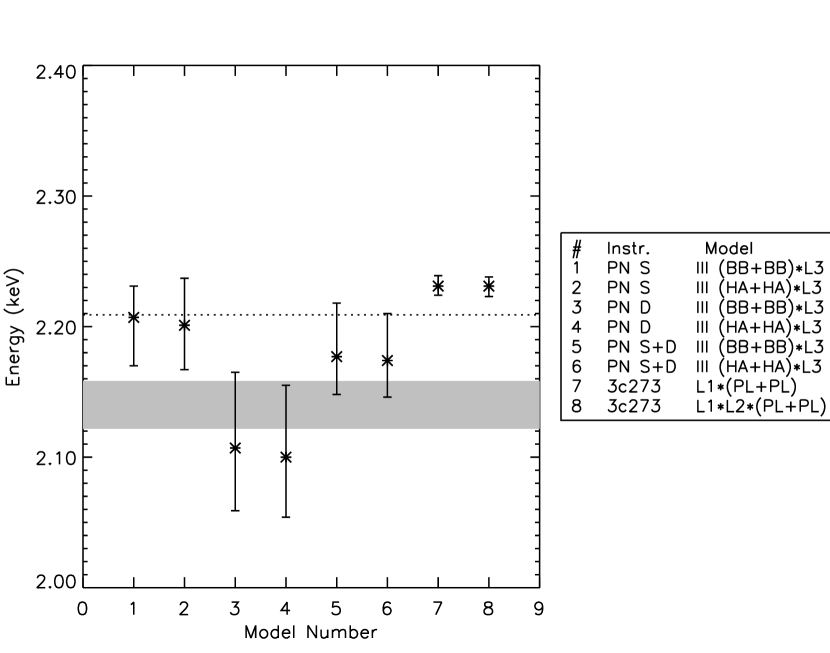
Figure 6: Line energy of a fitted 3rd line. The shaded region indicates the 90% confidence level found by DL04. All error bars are 68% confidence. The dotted line is at Au–M5 edge position.

6.2 Consistency test between PN and MOS data

In DL04 a large inconsistency ($\sim 5\sigma$) between the significance of the lines detected in PN and MOS data was reported, despite fit parameters being in statistical agreement. They explained this as being due to low energy calibration uncertainties in the MOS. This observation motivated us to perform a consistency check on our data set. Because we utilized a MOS energy cut slightly higher in energy, one would reduce low energy calibration uncertainties, and thus better consistency between MOS and PN data sets. This is what we have found, as described below.

We set up a Monte-Carlo simulation to test whether the 3rd line residual detected by PN could have appeared in MOS data as a deficit with a significance comparable to that observed. We used the III(BB+BB)*L3 model fit to the data because it showed the largest significance of a 3rd feature, therefore the largest discrepancy between PN and MOS. Hereafter we describe our formalism using PN-single and MOS1 case as an example: (1) we fit the model III(BB+BB)*L3 to the PN-single data and calculate best-fit parameters (2) we fold the model with variance in both the continuum and line parameters through MOS1 detector response and simulate a spectrum with the same exposure time and spectral bins as our analysis of the real data. (3) we evaluate $\Delta\chi^{2}$ by fitting a simulated spectrum with and without a 3rd line. We repeat this procedure 1000 times and compute the distribution of $\Delta\chi^{2}$. Figure 7 shows the results from the consistency test between PN and MOS1 (left) and PN and MOS2 (right).

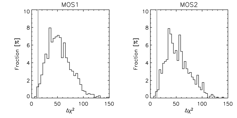
Figure 7: Results from the consistency test for PN-single data. The grey lines correspond to the measured $\Delta\chi^{2}$ values in MOS1 and MOS2 data.

We calculated the fraction of simulated $\Delta\chi^{2}$ points smaller than or equal to the measured $\Delta\chi^{2}$ ($S$), i.e. $f(\Delta\chi^{2}\leq S)$. The results are $f(\Delta\chi^{2}\leq S)=2.9\times 10^{-2}$ (MOS1) and $f(\Delta\chi^{2}\leq S)=3.1\times 10^{-2}$ (MOS2). The PN and MOS1 results are just consistent at the $1.90\sigma$ level and at the $1.86\sigma$ level between PN and MOS2. We conclude that the behavior of PN and MOS instruments is internally consistent with regards fitting of the lines, as we showed previously was the case for the continuum fits.

6.3 Strength of the residuals in the Au–M region

There are no statistically significant additional spectral features in the 1E1207 spectrum. For thoroughness we indicate just how weak the residuals are that we have uncovered at the Au-M edge. We do this by considering the residuals relative to 3C273, where the same instrument residuals are well-established (Kirsch, 2004).

We extracted PATTERN 0–4 events from a 40” radius region centered on the source. We used a double power law continuum model to fit the PN singles data in the 0.3–6.0 keV energy range. We did not fit the Au–M region but instead fit our model III with blackbody spectra for 1E1207 and double power-law continuum for 3C273, and plot the ratio of the residuals to the model spectrum (figure 8). We note that the residuals are $\sim$ 6–7% in the quasar data and $\sim$ 10–15% in the neutron star data. The neutron star data has larger error bars.

We directly calculated the EW of the 2.2 keV residuals without a line fit, and find them to be $\sim$ 40 eV. This is consistent with the EW we determined by line fitting. A similar calculation (as a sanity check) gave us 8 eV for the EW residuals at 2.2 keV in 3C273, in agreement with measurements of the XMM-Newton team (Kirsch, 2004). Of course the much higher noise level in the 1E1207 data renders the residuals insignificant. In figure 8 we show the ratio between the continuum model and the data for 1E1207. The same plot is shown for 3C273. We see there is nothing extraordinary in the NS data. The fluctuations are uniform through the entire spectrum. In 3C273 the Au-M edge is readily apparent because of the better counting statistics.

We note that a common error in estimating residual strength is to fit absorption lines and a continuum, and then to use the resultant continuum without lines as a basis for comparison with the residuals. This procedure grossly overestimates the continuum, and thus the strength of any absorption features with respect to it. The correct procedure of comparing the dips with respect to the best fit continuum markedly reduces the significance of the residuals. With this proper procedure our results here are consistent with those we obtained in §4.

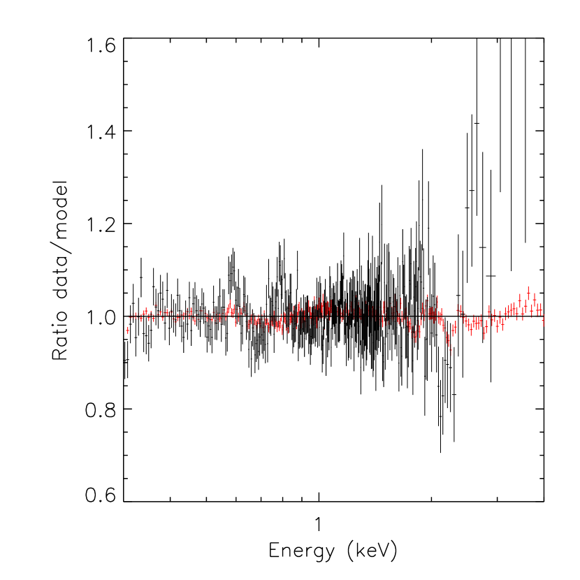
Figure 8: Data/model ratio plot for 1E1207 (black) and 3c273 (red).

7 Conclusions

• Utilizing a wider range of physically plausible INS models and careful background subtraction we have obtained continuum fits for 1E1207 which effectively rule out the need for additional harmonics of the first two spectral absorption features. Our derived continuum parameters for both PN and MOS data are consistent with those found by previous investigators.

• To explore the significance of the weak residuals found at higher energies in a few cases, we have implemented an improved F-statistic analysis for additional weak lines in 1E1207. It corrects for systematic overestimation of absorption line strengths using the standard F-test, as previously reported in the literature. Calculating the correct, finite statistics reference distribution for the F-statistic we find lines at harmonics of the two firmly established lines are statistically insignificant.

• We performed three completely independent statistical analyses to test for the presence of third and fourth spectral features. All tests give consistent results and all tests indicate there is no third or fourth line.

• While there are no statistically significant spectral features at higher energies, we explicitly fit the spectral residuals around 2.1 keV. Using the continuum model favored by previous investigators, and for which we get excellent continuum fits, we find the PN single spectrum residuals occur at the position of the instrumental Au-M edge. The residuals appear at the same energy as those obtained by fitting the known Au-M residuals in 3C273 with the identical procedure. We further show that PN doubles events yield a much lower energy for the residuals, as does the combined PN singles/doubles data set. This is highly suggestive of an instrumental origin for the insignificant residuals. Indeed in all eight physically plausible INS models we considered, the residuals always appear at the Au-M edge.

• We have demonstrated that the strength of the weak instrumental residuals in the 1E1207 spectrum are consistent with the stronger instrumental residuals observed in the 3C273 spectrum.

Appendix A Testing for a spectral line in a continuum

Some important results used in §4.2 are summarized here. The arguments of Eadie et al. (1983) are closely followed.

Consider searching a region of interest (ROI) consisting of $K$ bins for a deficit of counts over the expected continuum. The total spectrum has $N$ bins. Define $b_{i}$ as the true continuum, $\hat{b_{i}}$ as the estimated continuum, and $n_{i}$ as the observed counts in bin $i$. We can define the difference of counts in bin $i$ as $s_{i}=n_{i}-\hat{b_{i}}$.

The search for residual in the $K$ bins of the ROI can be formulated as a goodness-of-fit test, and under the null hypothesis $H_{0}$ there are no residuals, and $E(s_{i})=E(n_{i})-\hat{b_{i}}=b_{i}-\hat{b_{i}}\simeq\hat{b_{i}}-\hat{b_{i}}=0$, where $E$ is the expectation (mean) operator. A reasonable test statistic is $T=\sum_{i=1}^{K}\frac{(n_{i}-\hat{b_{i}})^{2}}{V(n_{i}-\hat{b_{i}})}$ where $V()$ is the variance operator. This statistic is a function of the random variables $z_{i}=\frac{n_{i}-\hat{b_{i}}}{\sqrt{V(n_{i}-\hat{b_{i}})}}$.

The $z_{i}$ have the following properties if $H_{0}$ is true. $E(z_{i})=0$, and $V(n_{i}-\hat{b_{i}})=V(n_{i})+V(\hat{b_{i}})-cov(n_{i},\hat{b_{i}})=V(b_{i})+V(\hat{b_{i}})=\hat{b_{i}}+\hat{\sigma_{i}}^{2}$. $cov()$ is the covariance operator. The trick is that the $\hat{b_{i}}$ should be estimated using the $N-K$ bins outside the ROI, for then $n_{i}$ and $\hat{b_{i}}$ are uncorrelated and their covariance vanishes. The continuum is simply fit without utilizing the $K$ bins in the ROI. Also note that $V(\hat{b_{i}})\equiv\hat{\sigma_{i}}^{2}$ can be directly obtained from covariance matrix of the continuum fit. Thus under $H_{0}$,

$$T=\sum_{i=1}^{K}\frac{(n_{i}-\hat{b_{i}})^{2}}{\hat{b_{i}}+\hat{\sigma_{i}}^{2}}=\sum_{i=1}^{K}z_{i}^{2}$$ (A1)

and $E(z_{i})=0,V(z_{i})=1$. Thus the $z_{i}$ are standard, normal variables (for $s_{i}$ not too small), and $P(T)$ is a $\chi^{2}$ distribution with $K$ degrees of freedom.

For $K\>\vbox{\hbox{$>$\hskip-7.5pt\lower 4.30554pt\hbox{$\sim$}}}\>30$ we can simplify this result by defining a new statistic $y=\frac{T-K}{\sqrt{2K}}$. Since the mean and variance of the $\chi^{2}$ distribution are $K$ and $2K$ respectively, $y$ has a standard, normal distribution. Then as described in the text we can test $H_{0}$ by simply calculating $y$ and if $y<y_{c}=4$ we accept $H_{0}$.

Table 1: Best-fit continuum parameters to PN data

	PN	PN	PN	PN	PN	PN
	I(BB+BB)	II(BB+BB)	III(BB+BB)	I(HA+HA)	II(HA+HA)	III(HA+HA)
$N_{H}$ [$10^{22}$ cm2]	$0.126_{-0.017}^{+0.009}$	$0.128_{-0.005}^{+0.017}$	$0.132_{-0.014}^{+0.012}$	$0.146_{-0.009}^{+0.009}$	$0.151_{-0.010}^{+0.010}$	$0.155_{-0.016}^{+0.007}$
$kT^{\infty}_{S}$ [keV]	$0.159_{-0.005}^{+0.009}$	$0.154_{-0.017}^{+0.010}$	$0.153_{-0.009}^{+0.015}$	$0.116_{-0.009}^{+0.009}$	$0.109_{-0.006}^{+0.006}$	$0.116_{-0.007}^{+0.009}$
$R^{\infty}_{S}$ [km]	$5.01_{-0.36}^{+0.88}$	$5.3_{-0.5}^{+1.3}$	$5.51_{-0.87}^{+0.72}$	$21.2_{-3.7}^{+1.9}$	$23.7_{-2.5}^{+3.5}$	$21.2_{-3.9}^{+1.4}$
$kT^{\infty}_{H}$ [keV]	$0.296_{-0.012}^{+0.010}$	$0.287_{-0.020}^{+0.018}$	$0.286_{-0.010}^{+0.024}$	$0.358_{-0.057}^{+0.074}$	$0.316_{-0.040}^{+0.017}$	$0.360_{-0.064}^{+0.060}$
$R^{\infty}_{H}$ [km]	$0.97_{-0.12}^{+0.13}$	$1.09_{-0.23}^{+0.19}$	$1.10_{-0.28}^{+0.19}$	$0.68_{-0.28}^{+0.40}$	$1.01_{-0.24}^{+0.54}$	$0.67_{-0.23}^{+0.72}$
$E_{1}$ [keV]	$0.741_{-0.006}^{+0.008}$	$0.743_{-0.007}^{+0.007}$	$0.725_{-0.005}^{+0.006}$	$0.730_{-0.005}^{+0.005}$	$0.731_{-0.005}^{+0.005}$	$0.728_{-0.005}^{+0.005}$
$\tau_{1}$	$0.92_{-0.07}^{+0.05}$	$0.99_{-0.10}^{+0.26}$	$0.60_{-0.03}^{+0.06}$	$0.56_{-0.02}^{+0.02}$	$0.58_{-0.01}^{+0.02}$	$0.53_{-0.03}^{+0.02}$
$FWHM$ [keV]	$0.303_{-0.026}^{+0.024}$	$0.297_{-0.022}^{+0.015}$	$0.290_{-0.020}^{+0.030}$	$0.272_{-0.018}^{+0.023}$	$0.262_{-0.016}^{+0.017}$	$0.264_{-0.019}^{+0.020}$
$E_{2}$ [keV]	$1.398_{-0.010}^{+0.009}$	$1.382_{-0.009}^{+0.008}$	$1.388_{-0.008}^{+0.008}$	$1.391_{-0.008}^{+0.008}$	$1.379_{-0.008}^{+0.008}$	$1.389_{-0.009}^{+0.008}$
$\tau_{2}$	$2.9_{-1.2}\tablenotemark{b}$	$0.58_{-0.10}^{+0.16}$	$0.39_{-0.02}^{+0.04}$	$0.55_{-0.07}^{+0.05}$	$3.7_{-2.0}^{+13}$	$0.39_{-0.04}^{+0.04}$
$FWHM$ [keV]	$0.15_{-0.10}^{+0.02}$	$0.183_{-0.013}^{+0.026}$	$0.187_{-0.025}^{+0.026}$	$0.190_{-0.024}^{+0.027}$	$0.140_{-0.052}^{+0.029}$	$0.187_{-0.023}^{+0.028}$
$\chi^{2}/dof$	$0.98$	$0.98$	$0.99$	$0.98$	$0.98$	$0.98$
$dof$	$422$	$422$	$422$	$422$	$422$	$422$

Note. — For hydrogen atmosphere models, we fixed neutron star mass and radius to 1.4 $M_{\odot}$ and 10 km. $kT^{\infty}$ and $R^{\infty}$ are insensitive to variation of $M$ and $R$ (Zavlin et al., 1998).

Note. — All parameters include a roundoff digit except when it would have required displaying a fourth digit after the decimal point.

Table 2: Best-fit continuum parameters to MOS data

Instrument	MOS1	MOS1	MOS2	MOS2
Model	III (BB+BB)	III(HA+HA)	III(BB+BB)	III(HA+HA)
$N_{H}$ [$10^{22}$ cm2]	$0.05_{-0.04}^{+0.10}$	$0.176_{-0.037}^{+0.035}$	$0.075_{-0.053}^{+0.074}$	$0.182_{-0.050}^{+0.011}$
$kT^{\infty}_{S}$ [keV]	$0.197_{-0.027}^{+0.026}$	$0.117_{-0.016}^{+0.025}$	$0.204_{-0.030}^{+0.021}$	$0.123_{-0.020}^{+0.018}$
$R^{\infty}_{S}$ [km]	$3.4_{-1.2}^{+1.5}$	$20.3_{-7.7}^{+9.8}$	$3.0_{-0.8}^{+1.6}$	$18_{-6}^{+19}$
$kT^{\infty}_{H}$ [keV]	$0.374_{-0.040}^{+0.074}$	$0.41_{-0.06}^{+0.11}$	$0.373_{-0.039}^{+0.056}$	$0.418_{-0.063}^{+0.083}$
$R^{\infty}_{H}$ [km]	$0.39_{-0.17}^{+0.27}$	$0.49_{-0.20}^{+0.46}$	$0.37_{-0.17}^{+0.38}$	$0.43_{-0.17}^{+0.59}$
$E_{1}$ [keV]	$0.700_{-0.031}^{+0.033}$	$0.728_{-0.016}^{+0.013}$	$0.718_{-0.046}^{+0.018}$	$0.729_{-0.016}^{+0.013}$
$\tau_{1}$	$0.90_{-0.22}^{+0.52}$	$0.62_{-0.05}^{+0.12}$	$0.68_{-0.12}^{+0.49}$	$0.56_{-0.06}^{+0.09}$
$FWHM$ [keV]	$0.43_{-0.08}^{+0.22}$	$0.330_{-0.031}^{+0.043}$	$0.39_{-0.06}^{+0.15}$	$0.319_{-0.037}^{+0.056}$
$E_{2}$ [keV]	$1.418_{-0.010}^{+0.009}$	$1.417_{-0.009}^{+0.009}$	$1.403_{-0.009}^{+0.010}$	$1.402_{-0.009}^{+0.009}$
$\tau_{2}$	$0.46_{-0.05}^{+0.04}$	$0.39_{-0.05}^{+0.05}$	$0.47_{-0.05}^{+0.05}$	$0.44_{-0.04}^{+0.04}$
$FWHM$ [keV]	$0.236_{-0.038}^{+0.043}$	$0.181_{-0.030}^{+0.035}$	$0.229_{-0.037}^{+0.035}$	$0.215_{-0.031}^{+0.034}$
$\chi^{2}/dof$	$0.85$	$0.80$	$1.20$	$1.18$
$dof$	$139$	$139$	$137$	$137$

Note. — All parameters include a roundoff digit except when it would have required displaying a fourth digit after the decimal point.

Table 3: Goodness-of-fit parameters of 3rd line test

Continuum model	Parameters	PN single	PN double	MOS1	MOS2
	$T_{c}$	112.8	71.38	65.26	65.26
III(BB+BB)	$T$	85.90	43.42	24.79	41.03
	$1-C$	$1.7\times 10^{-2}$	$5.4\times 10^{-2}$	$5.3\times 10^{-1}$	$3.1\times 10^{-2}$
	$T_{c}$	112.8	71.38	65.26	65.26
III(HA+HA)	$T$	80.45	42.62	20.47	34.68
	$1-C$	$3.3\times 10^{-2}$	$6.3\times 10^{-2}$	$7.7\times 10^{-1}$	$1.2\times 10^{-1}$

Note. — Model I and II show very similar results as model III.

Table 4: Summary statistics for 3rd feature significance

Instrument	Continuum model	$P(F)$ analysis	Goodness-of-fit test	EW analysis
	I (BB*L3+BB)	1.77	2.13	*
	I (BB+BB*L3)	3.29	2.13	2.07
	I (HA*L3+HA)	2.81	1.18	1.69
	I (HA+HA*L3)	2.84	1.18	1.96
PN-single	II (BB+BB*L3)	3.27	2.22	2.18
	II (HA+HA*L3)	2.55	1.69	1.85
	III (BB+BB)*L3	3.26	2.17	2.14
	III (HA+HA)*L3	3.12	1.83	1.88
	I (BB*L3+BB)	0.70	0.33	*
	I (BB+BB*L3)	2.09	0.33	1.92
	I (HA*L3+HA)	0.32	-0.92	#
	I (HA+HA*L3)	0.32	-0.92	#
MOS1	II (BB+BB*L3)	2.36	0.28	1.82
	II (HA+HA*L3)	1.02	-0.83	#
	III (BB+BB)*L3	2.55	-0.07	1.36
	III (HA+HA)*L3	1.32	-0.73	#
	I (BB*L3+BB)	0.69	1.78	*
	I (BB+BB*L3)	2.21	1.78	1.65
	I (HA*L3+HA)	0.27	1.05	#
	I (HA+HA*L3)	-1.43	1.05	#
MOS2	II (BB+BB*L3)	2.17	1.97	1.68
	II (HA+HA*L3)	1.14	1.37	#
	III (BB+BB)*L3	2.14	1.87	1.87
	III (HA+HA)*L3	1.11	1.18	#

References

- Bevington (1969) Bevington, H. A. 1969, Data Reduction and Error Analysis for the Physical Sciences (New York: McGraw-Hill)
- Bignami et al. (2003) Bignami, G. F., Caraveo, P. A., Luca, A. D., & Mereghetti, S. 2003, Nature, 423, 725
- De Luca et al. (2004) De Luca, A., Mereghetti, S., Caraveo, P. A., Moroni, M., Mignani, R. P., & Bignami, G. F. 2004, A&A, 418, 625
- Dermer & Sturner (1991) Dermer, C. D. & Sturner, S. J. 1991, ApJ, 382, L23
- Eadie et al. (1983) Eadie, W. T., Drijard, D., & James, F. E. 1983, Statistical methods in experimental physics (Amsterdam: North-Holland, 1983)
- Freeman et al. (1999) Freeman, P. E., Lamb, D. Q., Wang, J. C. L., Wasserman, I., Loredo, T. J., Fenimore, E. E., Murakami, T. & Yoshida, A. 1999, ApJ, 524, 772
- Giacani et al. (2000) Giacani, E. B., Dubner, G. M., Green, A. J., Goss, W. M., & Gaensler, B. M. 2000, AJ, 119, 281
- Haberl et al. (2003) Haberl, F., Schwope, A. D., Hambaryan, V., Hasinger, G., & Motch, C. 2003, A&A, 403, L19
- Haberl et al. (2004) Haberl, F., Zavlin, V. E., Trümper, J., & Burwitz, V. 2004, A&A, 419, 1077
- Hailey & Mori (2002) Hailey, C. J. & Mori, K. 2002, ApJ, 578, L133
- Ho & Lai (2003) Ho, W. C. G. & Lai, D. 2003, MNRAS, 338, 233
- Ho et al. (2003) Ho, W. C. G., Lai, D., Potekhin, A. Y., & Chabrier, G. 2003, ApJ, 599, 1293
- Lampton et al. (1976) Lampton, M., Margon, B., & Bowyer, S. 1976, ApJ, 208, 177
- Kirsch (2004) Kirsch, M. 2004, XMM-Newton EPIC status of calibration and data analysis (available at http://xmm.vilspa.esa.es/docs/documents/CAL-TN-0018-2-3.pdf)
- Mereghetti et al. (2002) Mereghetti, S., De Luca, A., Caraveo, P. A., Becker, W., Mignani, R., & Bignami, G. F. 2002, ApJ, 581, 1280
- Mori & Hailey (2003) Mori, K. & Hailey, C. J. 2003, submitted to ApJ, preprint (astro-ph/0301161)
- Protassov et al. (2002) Protassov, R., van Dyk, D. A., Connors, A., Kashyap, V. L., & Siemiginowska, A. 2002, ApJ, 571, 545
- Roe (1992) Roe, B. P. 1992, Probability and Statistics in Experimental Physics, Springer-Verlag, New York
- Romani (1987) Romani, R. W. 1987, ApJ, 313, 718
- Ruderman (2003) Ruderman, M. 2003, Proceedings of the 4th AGILE Science Workshop, preprint (astro-ph/0310777)
- Rutledge et al. (2002) Rutledge, R. E., Bildsten, L., Brown, E. F., Pavlov, G. G., & Zavlin, V. E. 2002, ApJ, 577, 346
- Sanwal et al. (2002) Sanwal, D., Pavlov, G. G., Zavlin, V. E., & Teter, M. A. 2002, ApJ, 574, L61
- Serfling (1980) Serfling, R. J. 1980, Approximation Theorems of Mathematical Statistics (New York: Wiley)
- Turbiner & López Vieyra (2004) Turbiner, A. V. & López Vieyra, J. C. 2004, Modern Physics Letters A, 19, 1919
- van Dyk et al. (2001) van Dyk, D. A., Connors, A., Kashyap, V. L., & Siemiginowska, A. 2001, ApJ, 548, 224
- van Kerkwijk et al. (2004) van Kerkwijk, M. H., Kaplan, D. L., Durant, M., Kulkarni, S. R., & Paerels, F. 2004, ApJ, 608, 432
- Wang et al. (1998) Wang, F. Y.-H., Ruderman, M., Halpern, J. P., & Zhu, T. 1998, ApJ, 498, 373
- Zavlin et al. (1996) Zavlin, V. E., Pavlov, G. G., & Shibanov, Y. A. 1996, A&A, 315, 141
- Zavlin et al. (1998) Zavlin, V. E., Pavlov, G. G., & Trumper, J. 1998, A&A, 331, 821