The X-ray Jet of 3C 120: Evidence for a Non-standard Synchrotron Spectrum

Abstract

We report on archival data from the Chandra X-ray Observatory for the radio jet of 3C120. We consider the emission process responsible for the X-rays from 4 knots using spectra constructed from radio, optical, and X-ray intensities. While a simple synchrotron model is adequate for three of the knots, the fourth (’k25’), which was previously detected by ROSAT and is now well resolved with Chandra, still represents a problem for the conventional emission processes. If, as we argue, the flat X-ray spectra from two parts of k25 are synchrotron emission, then it appears that either the emission comes from an electron distribution spectrally distinct from that responsible for the radio emission, or at the highest electron energies, there is a significant deviation from the power law describing the electron distribution at lower energies.

1 Introduction

3C120 is a nearby (z=0.033) radio galaxy which has variously been classified as a Seyfert 1, a broad line radio galaxy, and a late type spiral. The optical appearance is complex, with multiple dust lanes and two suggestive spiral arms which become radial features at a projected distance of 6.3 kpc from the core (fig. 1). The radio morphology and luminosity are more similar to the FRI class radio galaxy (Fanaroff & Riley 1974) than to the usual Seyfert. A one sided pc scale jet has been extensively studied with long baseline interferometry and superluminal components have been identified (apparent speeds between 3 and 6c, Walker et al. 2001). The kpc scale jet is shown in fig. 2 and there is additional complex emission at larger scales (beyond the borders of fig. 2, Walker, Benson, & Unwin 1987).

At X-ray wavelengths, the nucleus is a strong and variable source (e.g. Halpern 1985), but it was the detection with ROSAT of a rather inconspicuous radio knot 25^′′ from the core (16 kpc, projected), which presented new problems for the conventional models of X-ray emission from radio jets (Harris et al. 1999; HHSSV hereafter). Therefore we obtained new radio data at higher frequencies to see if this knot was peculiar or unique either in shock structure (as manifest by gradients in radio surface brightness) or in radio spectra. Now that Chandra data are in the archive, we have additionally studied the inner jet as well as being able to resolve the 25^′′ knot, so that we separate X-ray components by their morphology, and then test the various emission models.

The following sections describe the observations, data reduction, and photometry (2), the radio results (3), the X-ray emission processes (4), and an evaluation of each detected X-ray feature (5). We label the knots in the jet which are of primary interest, by their distance from the core in arcseconds (e.g. ’k4’, ’k25’). We take the distance to 3C 120 to be 140 Mpc (H_o=71 km s^-1 Mpc^-1; Spergel et al. 2003) so that 1” corresponds to 0.64 kpc. We use the standard definition of spectral index, $\alpha$: flux density, S${}_{\nu}\propto\nu^{-\alpha}$.

2 The observations and reduction procedures

2.1 The Radio Data

Details of the observations used in this paper are presented in Table 1. A comprehensive set of VLA and VLBI images between 1.4 and 15 GHz was published by Walker, Benson, and Unwin (1987). Here we use the 1983 October 2 VLA A-configuration image from that paper as the source of our 1.4 GHz flux densities. An extremely high dynamic range image of 3C 120 at 5 GHz was produced by Walker (1997) as a byproduct of an effort to measure the proper motion of the 4″ knot. We use that image, which is actually the weighted sum of 3 images widely separated in time (no variability in the jet was detected), to measure our 5 GHz flux densities.

To obtain good images at appropriate resolution at higher frequencies, we observed 3C120 at 14.9 GHz using the VLA B-configuration (second largest) and at 22.2 and 43.3 GHz using the VLA D-configuration (smallest). Both 22.2 and 43.3 GHz were observed with subarrays because 43.3 GHz was only available on 12 antennas. The 22.2 GHz image has inadequate resolution for use in this project and will not be presented. Reference pointing was used to keep 3C120 positioned properly in the VLA primary beams at 43 GHz. Because we were interested in the knot offset by 25″ from the core, and the VLA primary antenna beam is only about an arcminute FWHM at 43 GHz, we offset the pointing position by 12″ in the direction of the knot at that frequency. For all images, baseline based corrections for closure errors were made using scans on the bright, compact source 3C 84. The procedure is described in the above references.

All of the VLA images were calibrated following the normal procedures as described in the VLA Calibrator Manual. For all observations, the VLA continuum system was used with 50 MHz in each of two polarizations in each of two channels (200 MHz total). All data reduction was done using the NRAO Astronomical Imaging Processing System (AIPS). A primary beam correction was made for the 15 and 43 GHz images. At 43 GHz, that correction took into account the offset pointing position.

The measured flux densities for each of the features of interest are presented in Table 2 along with the optical and X-ray values. We estimate that the errors in our measured flux densities of strong features are 10, 5, 6, and 10% at 1.4, 5, 15, and 43 GHz, respectively. To this we add the image noise times the square root of the number of beam areas over which a given flux density is measured. The radio flux densities were measured in exactly the same boxes from each of the radio images although these rectangles, aligned with RA and DEC, are not identical to those used for optical and X-ray photometry. This is not thought to be a significant source of error since we ensured that the same features were being measured on the basis of radio overlays.

The resolutions of the images fall between 0.36″ and about 2″. Normally it is a poor idea to use interferometric images with unmatched resolutions for the measurement of flux densities from which spectra are to be derived. But in this case, there is no large scale structure in the regions of interest that is likely to show up in some images and not in others. The high resolution images are of high quality so all the flux density that would be seen at lower resolution should be present. As a result, we do not consider the mismatched resolutions to be a significant limitation. In fact, the normal effect of such a mismatch would be to have too little flux density measured in the higher resolution images. An examination of the spectra shows that, if anything, the opposite situation exists here.

2.2 The optical data

We retrieved an HST image of 3C120 from the WFPC2 Associations website. The selected file was taken from the F675W filter with a pivot wavelength of 6717 Å. We registered the data so as to align the optical and radio peak intensities (0.72^′′ shift). For the HST data, the peak position was found by the intersection of the diffraction spikes. After constructing a flux map (fig. 1) we measured the features of interest: k4, k7, s2, s3, and k25inner. The other parts of k25 were off the edge of the image, as was k80.

Uncertainties were estimated by using the same regions on the events image. For both sets of measurements we used ’funtools’. For k4, which lies on a relatively bright optical spiral like feature, we used a circular aperture significantly smaller than that used in the radio and X-ray bands (r=0.273^′′), chosen so as to include all of the obvious optical emission of k4. For the background, we chose the same size circle, positioned just to the North of k4 where the brightness was judged to be about the same as that surrounding k4. Note however, that this subjective choice means that the actual uncertainty in the flux of k4 is larger than the statistical error quoted in Table 2.

For the remaining features we used the same regions as defined for the X-ray photometry, except that we used a different background region for k25inner since the original background region was off the image. The resulting flux densities are given in Table 2.

For k25in which is close to the edge of the image, we found -58 counts in the source region (the background was oversubtracted), but +40 and +58 counts in two equally sized rectangles above and below the source. Thus we take $\sigma$ to be about the measured flux value: 0.34$\times 10^{-29}$ (cgs). For an upper limit, we take 3 $\sigma$ or 1 $\mu$Jy.

2.3 The X-ray Data

The archival Chandra data analyzed consist of an ACIS-S imaging observation (obsid 1613) and the zeroth order of an HETG observation (obsid 3015). The detectors are described in the CHANDRA Proposer’s Observatory Guide and the parameters of the observations are given in Table 3.

The imaging data were badly saturated at the core position, whereas the zero order image of the HETG data did not suffer from this problem: the so called “level 1” event file had a peak intensity pixel of 4940 counts (0.086 c/s, or 0.28 c/frame-time). Thus there is some pileup, but no saturation. The imaging observation also was done with a roll angle that made the readout streak fall on the inner jet (out to k4 and k7), but k25 was not affected. For these reasons, most of our results are based on the zero order image.

Our basic data reduction follows the procedures we used for M87 data (Harris et al. 2003). After checking the background for particle flares (our primary dataset was clean, and we decided not to exorcise the high countrate segment of 1613), we removed pixel randomization and registered the event file so that the x-ray and radio cores were aligned. This process for 1613 was problematic since the location of the X-ray core had to be estimated from the readout streak in one dimension, and for the orthogonal direction, an alignment of a circle with the wings of the central count distribution.

We then created 1024 arrays binned into 1/10 native ACIS pixel for each of four energy bands; constructed monochromatic exposure maps for an energy near the center of each band; and produced ’flux maps’ with units of ergs cm^-2 s^-1 by dividing the data by the exposure map and multiplying by the nominal h$\nu$ of the band. The exposure maps were generated using the time dependent effective area files which deal with the buildup of contamination on the ACIS detector. An example of a flux map is shown in fig. 3 with the regions overlayed.

Flux measurements consisted of choosing appropriate regions for jet features and corresponding backgrounds (see table 4 and fig.3); measuring the flux; and correcting for the mean energy (via the same source region, but operating on the event file). Since the flux maps were constructed with a multiplicative factor of h$\nu_{nominal}$, the correction factor of $<E>/E_{nominal}$ for each measurement is required to recover the actual flux within the band. In Table 5 we give the counts and flux for each jet component of interest.

Conversion of flux to flux density was done for an assumed power law with $\alpha$=1. Although this procedure is not strictly correct, the error introduced by using an incorrect value of $\alpha$ should be of second order since the bands were only a few keV wide. In general, we did not have enough counts to obtain an accurate value of $\alpha_{x}$, and for the brighter features such as k4, $\alpha_{x}$ is not far from 1.

Quoted uncertainties in fluxes and flux densities are purely statistical. They were derived by using the source and background regions on count maps (i.e. before dividing by the exposure maps). The fractional error in each flux was then carried forward to the flux densities.

Since most features do not have sufficient counts to provide an accurate estimate of the spectral parameters using the normal fitting procedures in the X-ray band, we use our measurements of flux densities (Table 2 ) to construct spectra (see sec. 5 for examples). Except for the uncertainty in the absorption correction for the softest band, we believe that our technique of deriving spectral parameters from the flux maps is reliable. For the case of k4 there are sufficient counts to allow the usual X-ray method of spectral fitting. We did that with Ciao/Sherpa and find agreement between the two methods, both in values of the amplitude and $\alpha_{x}$.

3 Results from the new radio data

We planned and obtained our new VLA radio data on the basis of the ROSAT observations of 3C 120. At that time a persistent question was “Why are a few knots and hotspots in radio jets detected with current X-ray sensitivities while the vast majority are not?” We now know that this question has been mostly answered because of the large number of jet detections with Chandra: with sufficient sensitivity and angular resolution, X-ray detections of radio jets are quite common and no longer drive us to search for ’special conditions’. However, it would still be useful to identify any peculiarities in shock regions containing electrons which produce significant X-ray emission. For k25 in particular, the difficulty of finding a reasonable emission mechanism for the X-rays led HHSSV to suggest the possibility of a flatter spectrum (than deduced from the radio data) population of relativistic electrons extending up to Lorentz energies of $\gamma\approx 10^{7}$.

For these reasons, we undertook high frequency VLA observations to better determine the radio spectrum and to evaluate the behavior of the sharp gradients in radio surface brightness at two locations in k25. Both of these parameters may be observational signatures of physical attributes of shocks.

3.1 Surface Brightness gradients

We used the AIPS tool NINER to measure the first derivative of the radio brightness. In order to measure comparative gradients at different frequencies, maps were convolved to the largest beamsize. However, when comparing different features on the same map, this convolution was not necessary.

For all comparisons we computed the normalized gradient by dividing the actual value of Jy/beam/pix by the intensity of the peak brightness of the feature being measured. When comparing maps with different pixel size, we also divided by the factor arcsec/pixel. In addition to measuring the gradient for the outer edge of k25, we measured gradients for the core (which serves to define the value for an unresolved source), k4, and the leading edge of k25 (which was undetected in our ROSAT data but is clearly present in the Chandra images).

3.2 Flux densities for spectra

To compare the spectra of the inner and outer shocks of k25, we measured flux densities on the Walker et al. (1987) maps constructed to have the same beamsize of 1.25$"$ FWHM (1.4, 5, and 15 GHz) and then repeated the measurements on maps smoothed to match the resolution of the 43 GHz map (2.2${}^{\prime\prime}\times 1.6^{\prime\prime}$) in order to include the 43 GHz flux density. We defined a rectangle of 3${}^{\prime\prime}\times 2.4^{\prime\prime}$ (RA$\times$DEC) for the internal (southern) shock and 2.4${}^{\prime\prime}\times 3^{\prime\prime}$ for the outer (western) shock. Although these integration areas are small, we corrected for background level by running IMEAN on a nearby region 15.6${}^{\prime\prime}\times 13.2^{\prime\prime}$. These corrections were $<$ 6% in all cases. The results are given in Table 2. The resulting spectral indices are $\alpha_{out}$ = 0.66$\pm$0.03 and $\alpha_{in}$ = 0.74$\pm$0.06.

3.3 Evaluation of Radio Results

There is no clear evidence for a significant difference in the spectral indices of the two parts of k25. The values are very close to each other and there are no data that demand a spectral break between 1.4 and 43 GHz. The outer shock structure is brighter than the inner feature at all frequencies we have measured.

Our attempts to measure the magnitudes of the gradients in the surface brightness have been less than rewarding. To make progress with this approach, it would be necessary to have a resolution and sensitivity at least equal to those of fig. 3. Our only indicative conclusion is that the ratio of the normalized gradients of the outer to the inner shock structures is greater than one at and below 5 GHz, and less than one above 10 GHz. However, the beamsizes employed even for this comparison are judged to be too large for any reasonable accuracy.

We conclude that there is very little or no difference between the two shocks (except for the total flux density) and neither is discernibly exotic. Given the ever increasing number of X-ray detections of radio jets, we take the absence of evidence for peculiarity in these putative shock features to be consistent with the idea that X-ray emission is relatively common for radio jets with a reasonable velocity towards us (i.e. two-sided X-ray jets are rare; we cannot cite even a single convincing example).

4 X-ray Emission Processes

In this section we discuss general aspects of the possible emission processes and for each jet feature tabulate the key parameters for each process. In section 5 we compare the processes for each feature in turn.

There are two basic problems: how to estimate the emitting volume (which influences the calculated value of the equipartition magnetic field strength) and what constraints might there be on the Doppler beaming factor, $\delta$ (which governs the IC calculations). In general, we have elected to use the largest reasonable volume, with the X-ray and highest resolution radio maps as a guide. Table 4 provides the dimensions and shapes of our assumptions. In some or possibly all cases the actual volumes may be smaller than that assumed, and that would lead to larger equipartition magnetic field strengths for synchrotron models or higher electron densities for thermal bremsstrahlung models.

To accommodate relativistic beaming from bulk jet fluid velocities ($\Gamma=(1-\beta^{2})^{-1/2}$; $\beta$=v/c), we will derive synchrotron parameters for a few representative values of $\delta=1/\Gamma(1-\beta~{}cos\theta)$ ($\theta$ is the angle between the jet direction and the line of sight). For thermal models we assume there is no beaming and for IC/CMB models we solve for the characteristic value of $\theta$ for which $\Gamma=\delta$.

4.1 Synchrotron models

We found no evidence that the outer shock in k25 is discernibly exotic in the radio (section 3), but from the X-ray morphology of k25, it is evident that the X-ray and radio emissions are co-spatial. This demonstrates that the suggestion of HHSSV, that the X-ray emission might originate in a much smaller volume than the radio emission, is not supported by the new data.

The synchrotron parameters listed in Table 6 are typical for FRI jets. With beaming, the intrinsic power of the source drops. Since we posit no change in emitting volume, the field drops as well. The halflife for electrons responsible for 2 keV emission ($\tau_{\frac{1}{2}}$) increases as the field drops, but eventually the IC losses dominate and so $\tau_{\frac{1}{2}}$ decreases. Since we have chosen to use the largest allowable emitting volume in each case, the actual value of the magnetic field strength may be larger than indicated, and this would decrease $\tau_{\frac{1}{2}}$.

The classical objection to the synchrotron model arises for those features which have an obvious inflection in their spectra to accommodate a flatter X-ray spectrum than would be anticipated by the segment connecting to optical or radio data. Two possible escapes from this objection are: (a) the existence of a distinct spectral component which is characterized by a flatter electron distribution so that its emission is below detection limits at frequencies below the X-ray band (as suggested for k25 by HHSSV), and (b) a scheme that leads to a ’pileup’ of electrons near the cutoff energy (e.g. Dermer & Atoyan 2002).

4.2 Beaming models

Inverse Compton emission from scattering on CMB photons by jet features with relativistic beaming has been suggested as a method to increase the energy produced via the IC channel relative to that in the synchrotron channel (Tavechhio et al. 2000; Celotti et al. 2001). Harris and Krawczynski (2002) calculated beaming parameters implied from the 3C 120 ROSAT data (HHSSV) if the jet components are in equipartition (energy density, u(particles) $\approx$ u(B)). With our revised values for the spectral indices and flux densities for several other features, we have recalculated the beaming parameters (Table 7).

The beaming parameters given in Table 7 are not entirely unreasonable if the $\Gamma$ of the jet does not decrease significantly out to k25. However, as noted in the table, for several features the spectral index observed in the X-ray band disagrees with that expected from the radio spectrum. Additionally, the small angles of the jet to the line of sight (of order 5^∘) for most of the knots, leads one to infer a large projection effect so that the physical size of the jet becomes rather long for an FRI. Furthermore, the beaming parameters required ($\Gamma,\delta,\theta$) are more extreme than those generally applied to the pc scale jet (Gomez et al. 2000; Walker et al. 1987).

A more general problem for the IC/CMB model is why the jet is not continuous in the X-rays once the emission ’starts’ with the generation of particles at a shock. Since we know the jet fluid continues downstream from a knot, the only way to quench the IC emission from the low energy electrons responsible for the X-rays, is to deflect the jet so that it is no longer pointing towards us, or to drastically reduce its velocity so that $\Gamma$ drops back close to one (in which case it would have to increase again at the next knot). For the synchrotron model, X-ray knots end quickly because of the large E² losses to the extremely high energy electrons required, but the very low energy electrons responsible for X-rays in the IC/CMB model have a very long half-life and thus should propagate undiminished for sizable segments of the jet. These and other difficulties of the IC/CMB models are discussed by Atoyan & Dermer (2004) and Stawarz et al. (2004). We believe the weight of the evidence argues against the IC/CMB model for the X-ray emission of the 3C120 jet.

4.3 Thermal Bremsstrahlung

Given the flat spectra found for a few features, we consider the possibility that the X-ray emission comes from hot gas (c.f. the interpretation for NGC 6251 by Mack, Kerp, & Klein 1997). For rough estimates of the parameters, we calculate the (uniform) density required to produce the observed X-ray flux. The results are given in Table 8.

The standard arguments against the thermal bremsstrahlung emission process include:

• if the X-ray emission occupies the same volume as the radio emission, there would be a departure from the $\lambda^{2}$ law for the radio polarization position angle;

• if the thermal region surrounds the emitting region, the predicted large rotation measures (RM’s) are not seen; and

• the thermal pressure of the emitting region generally exceeds the estimate of the ambient gas pressure.

At least for the inner jet, the observed RM’s are small (0 to -10 radians m^-2, Walker et al. 1987), so that the large RM’s of Table 8 would appear to preclude thermal X-ray emission. Reliable RM’s are not available for k25, but from polarization position angles at two frequencies for the brighter parts of k25, it seems likely that RM$\leq$100 rad  m^-2. No polarization data are available for k25new because of the very low radio brightness of this region so part, or conceivably all, of the X-ray emission from k25new could be from hot gas.

5 Evaluation of Features

5.1 The inner jet

As noted earlier, the X-ray image from the archival ACIS data without the grating is heavily saturated at the core position so that it is impossible to study the innermost region of the jet. Even the HETG zero order image has some degree of pileup, which means that the peak of the PSF is depressed relative to the wings. In spite of these difficulties, we constructed a PSF with ChaRT (the Chandra ray tracer) and subtracted it from the image. From a series of trial runs using different normalizations, we are convinced that there is substantial excess emission to the SW of the nucleus (and here we refer to the position of the radio nucleus since we registered all our files so as to align the radio and X-ray peaks). This emission lies between 0.5^′′ and 0.9^′′ from the nucleus at a PA of $\approx~{}225^{\circ}$; i.e. projected on the southern edge of the radio jet. An example of one of the residual maps is shown in fig. 4. Given the mismatch between the generated PSF and the data, we will not pursue the attributes of this feature here.

The X-ray emission from k4 is well resolved from the core region and aligns well with the corresponding optical and radio emissions (figs. 1 and 4). The values of the X-ray spectral index, $\alpha_{x}$, from spectral fitting (0.95$\pm$0.45) and from our 4 band fluxes (0.90$\pm$0.20) agree within the errors and are also consistent with the radio to X-ray index, $\alpha_{rx}$=0.90. Furthermore, the optical flux density falls on the power law defined by the radio and X-ray data. Thus we favor a synchrotron explanation (perhaps with modest beaming, e.g. $\delta$=3) for the X-ray emission. If the X-rays were to be beamed IC/CMB radiation, the apparently straight power law fit from radio and optical to X-rays would be a coincidence and $\delta$ would have to be $>$10 (Table 7). We note that while it appears that k4 lies in a spiral arm feature of the galaxy, we consider it highly probable that this is a coincidence. At the distance of 3C 120, 4^′′ corresponds to 2.5 kpc, a reasonable distance between the nucleus and a feature defined by stars. However, from VLBI studies of the superluminal radio jet, the angle between the jet and our line of sight is of order 5^∘, so k4 would be $\approx$ 29 kpc from the nucleus, and thus starlight would not be a viable source of photons for IC scattering.

The next knot, k7, has only 30 net counts so no spectral analysis was attempted. However, as shown in fig. 5, there is a significant difference between $\alpha_{rx}$=0.86 and $\alpha_{x}$=2.4$\pm$0.6, as derived from flux densities for 3 of our energy bands. This sort of spectrum is consistent with a power law distribution of relativistic electrons with a high energy cutoff (i.e. suffering E² energy losses); so again, we favor the synchrotron model. The 2$\sigma$ optical detection falls on the power law connecting the radio and X-ray data.

The next section of the jet (”s2” in fig. 3) is very weak in the X-rays and the following section, ”s3”, was not detected. However, the measurements are reported in Tables 2 and 5.

5.2 Knots k25 and k80

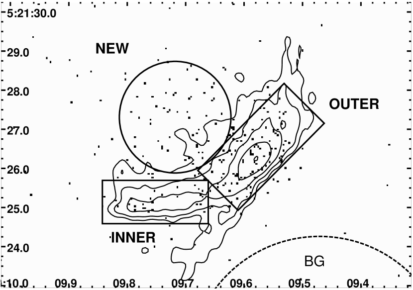
Figure 6: The events in the 0.5-10 keV band for k25. The radio contours are the same as used in fig. 3. The regions are shown as well.

The X-ray emission of k25 continues to be a problem insofar as the standard emission models are concerned (HHSSV). The new data make matters worse since we now find extended X-ray emission in a region of very low radio brightness. We call this region ’new’, and use the terms ’inner’ and ’outer’ for the two relatively bright radio edges which show large gradients in surface brightness: ’inner’ refers to the upstream edge and ’outer’ refers to the western edge. In fig. 6 we show the events comprising k25.

The only optical data we have is the upper limit to k25in, and this flux density lies well above the power law connecting the radio and X-ray flux densities. Note however that the optical upper limits quoted in HHSSV for the area then known to be associated with X-ray emission fall below the spectrum of the total emission, so the suspicion remains that it is not feasible to argue for a single power law from the radio to the X-ray. As shown in fig. 7, both the inner and outer regions have quite flat X-ray spectra, whereas $\alpha_{x}$ for the ’new’ region is consistent, within the errors, with $\alpha_{rx}$.

A flat power law ($\alpha_{x}$ close to zero) is normally not considered feasible as a synchrotron spectrum associated with standard shock acceleration expectations, but what are the alternatives?

Aside from the large beaming factor required for the IC/CMB model ($\delta>$10, Table 7), one would need to explain why the emission dies away moving downstream since the very low energy electrons responsible for IC/CMB should have very long halflives. The major unknowns for the IC/CMB model are the validity of extrapolating the electron spectrum down to the required low values of $\gamma$, and the actual value of the bulk relativistic velocity, i.e. $\Gamma$.

As shown in Table 8, thermal emission models encounter a number of problems and thus we do not believe that thermal bremsstrahlung is a viable alternative to synchrotron emission for the brighter regions, k25in and k25out.

For the synchrotron model, aside from the requirement for a separate spectral component with a flat spectrum, we face the difficulty of propagating high energy electrons from the acceleration sites (i.e. the inner and outer large-gradient radio features) to fill the enclosed volume (’new’). The required distance is of order 3^′′ (1.9 kpc in projection); a light travel time of some 6000 years. This may be compared with typical lifetimes of the highest energy electrons against E² losses (with equipartition magnetic field strengths) of $\approx$ 200 years (Table 6). If the X-ray emission from k25new is thermal (the anonymous referee suggested shocked gas), the travel time problem for high energy electrons would be moot.

An alternative explanation for the presence of high energy electrons in the ’new’ region would be distributed acceleration (i.e. not directly associated with obvious shocks), as might be the case for reconnection scenarios (Birk & Lesch 2000, Birk, Crusius-Wätzel, & Lesch 2001), or acceleration associated with turbulence along the jet edge (Stawarz et al. 2004, and references therein).

Knot k80 (fig. 2) is of low radio brightness, but we find associated X-ray emission. The morphological correspondence between radio and X-rays is not close as in the other 3 knots. In fig. 8 we show the relevant maps. Insofar as the detected structures are concerned, the situation of the X-rays being slightly displaced upstream of the bulk of the radio emission is very similar to that in the outer knot in the jet of PKS1127-145 (Siemiginowska et al. 2002). The three values of S_x in Table 2 are consistent with $\alpha_{rx}$=0.8. As for the inner knots, the results of section 4 leave little doubt that the x-rays come from synchrotron emission.

6 Conclusions

The X-ray emission from k25 remains a puzzle. The only ad-hoc models which we can suggest involve distinct spectral populations of relativistic electrons. For synchrotron emission, this would be a flat spectrum component extending to electron Lorentz factors of $\gamma=10^{7}$ to $10^{8}$ (see table 5 of HHSSV). Note however that “a distinct spectral population” need not indicate a separate shock region for its genesis. Dermer & Atoyan (2002) have described E² loss conditions which can produce spectral hardening at high energies near the cutoff, and Niemiec & Ostrowski (2004) have produced numerical simulations for what they call ’realistic’ magnetic field structures in relativistic shocks that can provide both relatively flat particle distributions and even flatter high energy tails for energies below the cutoff. For IC/CMB with beaming, the parameters derived above could be relaxed if an additional, steep spectrum distribution of electrons existed below $\gamma=2000$ (see section 5.2 of Harris and Krawczynski 2002). A 60ks observation with Chandra has been approved for AO6. When these data are available we should obtain more accurate X-ray spectral parameters.

Although one of us (DEH) has been a long and ardent supporter of the classical view: “If the spectrum is not concave downward, it is not synchrotron emission”, it is now our view that there is strong evidence for marked deviations from this scenario. It should be remembered at this point, that there are many other knots in jets for which $\alpha_{x}~{}<~{}\alpha_{ox}$, (e.g. NGC6251, Sambruna et al. 2004), and we believe it would be more fruitful to re-interpret these occurrences rather than to cite them as proof that synchrotron models are impossible.

7 References

Atoyan, A. & Dermer, C. D. 2004, (submitted to ApJ)

Birk, G. T. & Lesch, H. 2000 ApJ 530, L77

Birk, G. T., Crusius-Wätzel, A. R., & Lesch, H. 2001 ApJ 559, 96

Celotti, A., Ghisellini, G., & Chiaberge, M. 2001 MNRAS 321, L1

Dermer, C. D.& Atoyan, A. M. 2002 ApJ 586, L81

Gomez, J. L., Marscher, A. P., Alberdi, A., Jorstad, S. G., & Garcia-Miró, C. 2000, Science 289, 2317

Halpern, J. P. 1985 ApJ 290, 130.

Harris, D. E. and Krawczynski, H. 2002, ApJ 565, 244

Harris, D.E., Hjorth, J., Sadun, A.C., Silverman, J.D. & Vestergaard, M. 1999 ApJ 518, 213 (HHSSV)

Harris, D. E., Biretta, J. A., Junor, W., Perlman, E. S., Sparks, W. B., and Wilson, A. S. 2003 ApJ 586, L41.

Hjorth, J., Vestergaard, M., S$\o$rensen, A. N., & Grundahl, F. 1995 ApJ 452, L17

Mack, K.-H., Kerp, J., & Klein, U. 1997 A&A 324, 870

Niemiec, J. & Ostrowski, M. 2004 ApJ (in press)

Sambruna, R.M., Gliozzi, M., Donato, D., Tavecchio, F., Cheung, C.C., & Mushotzky, R.F. 2004, A&A, 414, 885

Siemiginowska, A., Bechtold, J., Aldcroft, T.L., Elvis, M., Harris, D.E., and Dobrzycki, A. 2002 ApJ 570, 543

Spergel, D. N. et al. 2003 ApJS 148, 175

Stawarz, L., Sikora, M., Ostrowski, M., & Begelman, M. C. 2004 ApJ (in press)
http://arXiv.org/abs/astro-ph/0401356

Tavecchio, F., Maraschi, L., Sambruna, R.M., & Urry, C.M. 2000 ApJL 544, L23-26

Walker, R.C., Benson, J.M., and Unwin, S.C. 1987 ApJ 316, 546

Walker, R.C. 1997 ApJ 488, 675

Walker, R.C., Benson, J.M., Unwin, S.C., Lystrup, M.B., Hunter, T.R., Pilbratt, G., & Hardee, P.E. 2001 ApJ 556, 756

Figure 1: The HST image used for photometry, with radio contours overlaid. Knot k4 is towards the right hand edge in this figure. The bright emission along the southern edge of the jet is part of the diffraction spike from the nucleus. The radio contours are the same as used in fig. 3. The WFPC2 image was taken with the F675W filter.

Figure 2: Radio contours at 1.6 GHz. This map from 1982 data (Walker et al. 1987) shows the section of the jet of interest, with several knots labelled. There are additional radio features on larger scales (see Walker et al. 1987). The beamwidth is 3.5^′′ FWHM; the first contour level is 0.25 mJy/beam and successive contours increase by factors of 2.

Figure 3: The 0.5 to 10 keV map of 3C120 with overlayed regions for measuring the flux. The X-ray data have been smoothed with a Gaussian of FWHM= 0.5^′′. Dashed regions are background regions. Radio contours from the VLA at 5 GHz (CLEAN beamwidth = 0.365”) are overlayed. Contour levels start at 0.05 mJy/beam and increase by factors of two. The regions are labelled by their distance from the core in arcsec for knots, and by ’s2’ and ’s3’ for smooth sections of the jet detected in the optical by Hjorth et al. (1995).

Figure 4: A residual X-ray map after subtraction of the PSF showing the excess emission to the southwest of the nucleus. The white contours are linear: 0.5, 1.0, 1.5, … 4.0 counts per 0.049^′′ pixel. An additional contour at -8 shows the location of the PSF subtraction. The black area in the center is negative, most likely caused by pileup suppressing the true peak intensity. The image was generated with an energy filter from 0.5 to 10 keV and smoothed with a Gaussian of FWHM=0.25^′′. Overlaid are light magenta radio contours from a 6cm VLA map with the lowest contour level at 0.2 mJy/beam and successive contours increase by factors of two. The beam is circular with FWHM=0.365^′′.

Figure 5: Spectra for components of the inner jet. The solid line (circles) is for k4; the dashed line (crosses), k7; and the dotted line (squares), s2. The down triangle is a 2 $\sigma$ (optical) measurement for k7. The optical values for k4 and s2 are so close to each other that their symbols overlap. The left panel shows the radio to X-ray spectrum; the right panel shows the X-ray data.

Figure 7: The spectra for the components of k25. The left panel shows the radio to X-ray spectrum; the right panel shows the X-ray data. The strongest feature is the outer region, crosses and solid line; the inner region is marked by circles and a dashed line; and the ’new’ region is denoted by squares and a dotted line. The up-triangle is an upper limit for k25in from HST, and the two down-triangles are upper limits reported by HHSSV for the total k25 optical emission.

Figure 8: The outer knot, k80. The X-ray images come from obsid 1613, consist of counts between 0.4 and 6 keV, and have been regrided to 1/4 native ACIS pixel. The left panel has been smoothed with a Gaussian of FWHM=1^′′; the right panel with a 2^′′ Gaussian. Radio contours are overlayed. Those on the left show just the brighter, more compact levels from a 5 GHz VLA observation with the B array: with a beamsize of 1.36${}^{\prime\prime}\times 1.13^{\prime\prime}$ in PA=44^∘, and contours at 0.15, 0.20, and 0.25 mJy/beam. The contours on the right panel are from a 1.5 GHz (B array) observation with a 3.8^′′ beam with the first contour at 0.2mJy/beam and successive contours increase by factors of two. There are between 6 and 9 counts in the two weak X-ray features upstream of k80. In both panels, the colors span a factor of 4 in X-ray brightness. The peak brightnesses are 0.038 (right) and 0.06 (left) counts per 0.123” pixel.

Figure 9: The spectrum of k80. The left panel shows the radio to X-ray spectrum; the right panel shows the X-ray data.

Table 1: VLA Observations

		Beam Size				Calibrators
Frequency	Date(s)	MajAx	MinAx	PA	Peak	rms	3C 286	3C 48
(GHz)		(″)	(″)	(Deg)	(Jy/beam)	(mJy)	(Jy)	(Jy)
(1)	(2)	(3)	(4)	(5)	(6)	(7)	(8)	(9)
1.45	1983 Oct. 2	1.26	1.25	47	2.76	1.45	14.51	$\cdots$
4.86	Multiple	0.365	0.365	$\cdots$	3.15	0.012	7.55	$\cdots$
14.94	2000 Jan. 4	0.54	0.51	24	3.36	0.033	3.43	1.80
43.34	Multiple	2.21	1.60	-2	2.07	0.25	1.45	0.575

Note. — The columns in the table give (1) the observing frequency, (2) the date(s) of the observations, the CLEAN restoring beam (3) major and (4) minor axis size (FWHM) and (5) position angle, (6) the peak flux density in the image (always on the 3C 120 core source which is highly variable), (7) the image off-source rms noise level, (8) the assumed flux density of 3C 286 used in the flux density calibration, and (9) the flux density of 3C 48 used in the calibration, when it was used.

Table 2: Flux Densities (ergs cm^-2 s^-1 Hz^-1) and Spectral Indices

Quantity	k4	k7	s2	s3	k25in	k25out	k25new	k80
S(1.5GHz)	1.4$\pm$0.1E-24	3.2$\pm$0.5E-25	1.5$\pm$0.4E-25	9.0$\pm$3.9E-26	1.2$\pm$0.4E-25	1.5$\pm$0.4E-25	$\cdots$	6.0$\pm$0.6E-26
S(5GHz)	6.6$\pm$0.3E-25	1.6$\pm$0.1E-25	8.4$\pm$0.4E-26	5.1$\pm$0.3E-26	4.3$\pm$0.2E-26	6.9$\pm$0.4E-26	9.1$\pm$1.5E-27	$\cdots$
S(15GHz)	2.8$\pm$0.2E-25	7.2$\pm$0.5E-26	3.9$\pm$0.3E-26	2.6$\pm$0.2E-26	2.5$\pm$0.2E-26	3.5$\pm$0.3E-26	$\cdots$	$\cdots$
S(43GHz)	1.2$\pm$0.1E-25	3.2$\pm$0.5E-26	1.6$\pm$0.5E-26	8.1$\pm$5.0E-27	0.9$\pm$0.5E-26	1.6$\pm$0.5E-26	$\cdots$	$\cdots$
S(4.47E14Hz)	2.7$\pm$0.3E-29	0.9$\pm$0.4E-29	2.6$\pm$0.4E-29	1.0$\pm$0.1E-29	$\cdots$	$\cdots$	$\cdots$	$\cdots$
S(2.42E17Hz)	1.0$\pm$0.2E-31	6.3$\pm$1.6E-32	$\cdots$	0.8$\pm$0.6E-32	1.7$\pm$0.9E-32	6.0$\pm$1.5E-32	5.5$\pm$1.4E-32	2.4$\pm$0.6E-32
S(6.05E17Hz)	5.8$\pm$1.0E-32	0.5$\pm$0.4E-32	0.5$\pm$0.3E-32	$\cdots$	1.3$\pm$0.4E-32	4.7$\pm$0.8E-32	2.5$\pm$0.6E-32	1.6$\pm$0.5E-32
S(9.67E17Hz)	3.8$\pm$0.8E-32	0.2$\pm$0.2E-32	$\cdots$	$\cdots$	1.4$\pm$0.5E-32	5.8$\pm$0.9E-32	2.4$\pm$0.5E-32	5.1$\pm$4.7E-33
S(1.69E18Hz)	2.7$\pm$1.1E-32	$\cdots$	0.2$\pm$0.1E-32	$\cdots$	1.5$\pm$0.7E-32	3.5$\pm$1.2E-32	1.0$\pm$0.6E-32	$\cdots$
Spectral Indexes
$\alpha_{r}$	0.74$\pm$0.04	0.68$\pm$0.04	0.67$\pm$0.06	0.69$\pm$0.10	0.74$\pm$0.06	0.66$\pm$0.03	$\cdots$	$\cdots$
$\alpha_{rx}$	0.90	0.86	0.97	$\cdots$	0.82	0.81	0.70	0.79
$\alpha_{x}$	0.90$\pm$0.20	2.4$\pm$0.6	0.2$\pm$0.6	$\cdots$	0.0$\pm$0.4	0.3$\pm$0.3	0.6$\pm$0.2	0.7$\pm$0.4

Table 3: Chandra observations

Obsid	Date	Detector	Grating	livetime	CALDB
				(sec)
1613	2001-09-18	ACIS-235678	none	12,881	2.8
3015	2001-12-21	ACIS-456789	HETG	57,218	2.10

Table 4: Specifics of the regions and assumed sizes for volumes

	Region Specification				Assumed Volumes
region	shape	RA(J2000)	DEC(J2000)	size	shape	dimensions	pathlength
				(′′)		(′′)	(kpc)
k4	circle	04:33:10.843	+05:21:15.09	0.738	sphere	0.33	0.42
k7	rotbox	04:33:10.628	+05:21:15.44	2.165, 1.427	sphere	0.33	0.42
s2	rotbox	04:33:10.450	+05:21:16.70	3.542, 1.230	cyl.	0.33;3.0	0.42
s3	rotbox	04:33:10.232	+05:21:18.35	3.444, 1.230	cyl.	0.33;2.8	0.42
k25in	rotbox	04:33:09.752	+05:21:25.14	2.706, 1.107	cyl.	0.33;2.1	0.42
k25out	rotbox	04:33:09.571	+05:21:26.55	3.132, 1.447	cyl.	0.6;1.8	0.76
k25new	circle	04:33:09.718	+05:21:27.31	1.427	sphere	1.43	1.82
k80	circle	04:33:07.937	+05:22:21.22	4.797	sphere	3.0	3.82

Table 5: X-ray fluxes (in units of 10^-14 erg cm^-2 s^-1) and source counts

Energy	k4	k7	s2	s3	k25in	k25out	k25new	k25tot	k80
0.5-1.5	1.85$\pm$0.39	1.16$\pm$0.27	$\cdots$	0.15	0.31$\pm$0.16	1.11$\pm$0.28	1.02$\pm$0.25	3.15$\pm$0.47	0.49$\pm$0.12
1.5-3	3.35$\pm$0.57	0.26$\pm$0.22	0.27$\pm$0.16	$\cdots$	0.77$\pm$0.25	2.72$\pm$0.49	1.43$\pm$0.36	6.03$\pm$0.72	0.50$\pm$0.17
3-6	2.55$\pm$0.56	0.15$\pm$0.12	$\cdots$	0.14	0.93$\pm$0.31	3.90$\pm$0.62	1.60$\pm$0.37	7.80$\pm$0.86	0.34$\pm$0.32
6-10	2.35$\pm$0.96	$\cdots$	0.16$\pm$0.10	$\cdots$	1.29$\pm$0.65	3.02$\pm$1.03	0.90$\pm$0.54	6.10$\pm$1.40	…
0.5-10	10.1$\pm$0.91	1.42$\pm$0.36	0.43$\pm$0.26	$\cdots$	3.30$\pm$0.99	10.7$\pm$1.07	4.95$\pm$0.64	23.08$\pm$1.62	1.33$\pm$0.39
Source Counts
Total counts	124	34	14	7	27	98	55	225	48
Net counts	121	29	7	0	22	90	44	215	37

Note. — Both observations were made with the standard CCD readout time of 3.2s.

Note. — Columns to the left describe the regions used for photometry except where noted in the text. The last 3 columns give the assumed geometry of the emitting volumes. The background regions are shown in fig. 3. All coordinates refer to the radio maps.

Table 6: Parameters for a Synchrotron Model

						$\delta=$3		$\delta=$6
Region	B(1)	$\alpha_{r}$	$\alpha_{rx}$	logLs	$\tau_{\frac{1}{2}}$	logLs	$\tau_{\frac{1}{2}}$	logLs	$\tau_{\frac{1}{2}}$
	($\mu$G)			(erg/s)	(years)	(erg/s)	(years)	(erg/s)	(years)
k4	116	0.74	0.9	41.83	23	39.92	56	38.72	27
k7	72	0.68	0.84	41.47	47	39.56	86	38.36	47
s2	33	0.67	0.97	40.62	152	38.73	108	37.53	17
k25inner	36	0.74	0.82	41.14	131	39.23	108	38.03	18
k25outer	27	0.66	0.81	41.45	195	39.54	105	38.34	16
k25new	9	$\cdots$	0.70	41.24	669	39.33	74	38.13	9
k80	8.3	$\cdots$	0.79	41.14	762	39.24	69	38.03	9

Note. — The emission spectrum is assumed to cover the range E6 to 5E18 Hz in the observed frame.

Table 7: Parameters for an Inverse Compton Model with Bulk Relativistic Velocities

Region	$\alpha$	B(1)	R(1)	$\delta$	$\theta$	R′	Distance
		$\mu$G		$\Gamma$	(deg)		(kpc)
k4	0.74	116	0.0917	16	3.5	65	42
k7	0.68	72	0.0176	12	4.5	56	57
s2	0.67	33	0.0104	7.7	7.5	40	49
k25in	0.74	36	0.3967	13	4.5	352	184
k25out	0.66	27	0.1939	18	3.2	1840	269
k25new	0.70	10	1.3454	14	4.1	5060	215
k80	0.79	8.3	0.6289	5.3	10.5	137	281

Table 8: Thermal Bremsstrahlung Parameters

Region	ne	Cooling Time	Mass	Pressure	RM
	(cm-3)	(years)	(M⊙)	(dyne cm-2)	(m-2)
k4	6.6	1.5E5	6.3E6	2.0E-8	22,450
k7	2.5	4.0E5	2.4E6	7.5E-9	8,500
s2	0.6	1.8E6	3.7E6	1.7E-9	2,040
k25inner	1.7	5.6E5	8.0E6	5.6E-9	5,780
k25outer	1.9	5.2E5	2.4E7	5.6E-9	11,450
k25new	0.5	1.9E6	4.0E7	1.5E-9	7,520
k80	0.08	1.2E7	5.9E7	2.5E-10	2,500