An xspec model to explore spectral features
from black-hole sources

Abstract

We report on a new general relativistic computational model enhancing, in various respects, the capability of presently available tools for fitting spectra of X-ray sources. The new model is intended for spectral analysis of black-hole accretion discs. Our approach is flexible enough to allow easy modifications of intrinsic emissivity profiles. Axial symmetry is not assumed, although it can be imposed in order to reduce computational cost of data fitting. The main current application of our code is within the xspec data-fitting package, however, its applicability goes beyond that: the code can be compiled in a stand-alone mode, capable of examining time-variable spectral features and doing polarimetry of sources in the strong-gravity regime. Basic features of our approach are described in a separate paper (Dovčiak, Karas & Yaqoob [9]). Here we illustrate some of its applications in more detail. We concentrate ourselves on various aspects of line emission and Compton reflection, including the current implementation of the lamp-post model as an example of a more complicated form of intrinsic emissivity.

1 Introduction

Regions of strong gravitational field are most usually explored via X-ray spectroscopy, because very hot X-ray emitting material is commonly believed to be present in regions near a neutron star surface or a black-hole horizon. Accretion plays crucial role in the process of energy liberation and mass accumulation that takes place in this kind of objects [16, 17]. In particular, disc-type accretion represents an important mode which is realized under suitable circumstances, given by the global geometrical arrangement and local microphysics of the fluid medium. A central compact body, undetectable via its own radiation, resides in galactic nuclei where it is surrounded by a rather dense population of stars and gaseous environment. Photons emerging from the accretion disc and its corona are influenced by gravity of the black hole, so they bear various imprints of the gravitational field structure. This concerns especially X-rays originating very near the core and, for this reason, spectral analysis with X-ray satellites is particularly relevant for astronomical study of strong gravitational fields around black holes. For a general discussion, see review articles [10, 27] and further references cited therein.

In this paper we describe a newly developed computational model aimed for the spectral analysis of line profiles and continuum originating in a geometrically thin, planar accretion disc near a rotating (Kerr) black hole. Such analysis has been routinely performed via xspec package [1], which performs deconvolution of observed spectra for the effective area and energy redistribution of the detector. Previously, several routines were developed and linked with this package in order to fit data to a specific model of a black-hole accretion disc [19, 20]. However, a substantially improved variant of the computational approach has been desirable because previous tools have various limitations that may be critical for analyses of present-day and forthcoming high-resolution data.

We describe the layout and usage of the new code and we show some examples and comparisons between new model components. Our present contribution provides information complementary to the basic description which can be found in ref. [9]. We suggest the reader to consult that paper as well as further details in Thesis [8], as they give more examples and citations to previous works. Here we concentrate our attention to technical issues of the code structure and its performance when computing and fitting spectra. Different perspectives and applications of general relativistic computations for black-hole accretion discs have been considered by various authors. In particular, it is very useful to consult recent papers of Gierliński, Maciolek-Niedźwiecki & Ebisawa [14] and Schnittman & Bertschinger [28]. Very recently, a new independent code has been developed by Beckwith & Done [2]. Their approach also allows to study accretion disc spectra including strong gravity effects of a Kerr black hole. This is also one of the applications of our code, and so relatively accurate comparisons between both tools are possible. We performed several such comparisons and found a very good agreement in the shape of predicted line profiles.

Given a limited space for this contribution, we cannot describe all aspects of the new code: capability of the code with respect to timing and polarimetry are discussed elsewhere. Nonetheless, it may be good to bear in mind that such capability has been already implemented and tested, taking into account all strong-gravity effects on time-delays and the Stokes parameters.

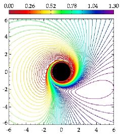
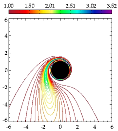
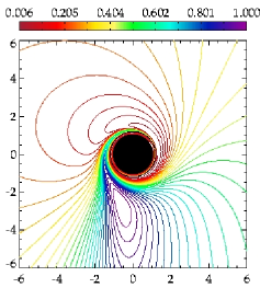
a) $g$-factor	b) lensing	c) cosine of the angle of emission
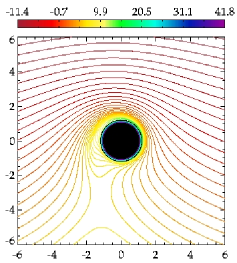
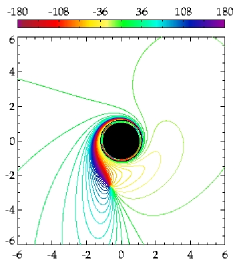
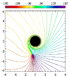
d) relative time delay	e) change of the angle of polarization	f) azimuthal emission angle

Figure 1: Six transfer functions are shown in the equatorial plane of a Kerr black hole with $a\doteq 0.9987$ (horizon $r_{\rm h}=1.05$). The black hole rotates counter-clockwise. The observer is located upwards at the inclination $\theta_{\rm o}=70^{\circ}$. The values of transfer functions are encoded by a colour scale, as indicated above each graph. For mathematical formulae defining these functions see eqs. (A65), (A66)–(A71) and (A78) in Appendix A.1.

2 Transfer functions

We concentrate on geometrically thin and optically thick accretion discs and we point out that general relativity effects can play a role if the configuration is sufficiently dense in a limited region, typically a few tens of gravitational radii. Nevertheless, our computational domain extends up to about $\approx 10^{3}$ gravitational radii in a non-uniform spatial grid.

In order to calculate the final spectrum that an observer at infinity measures when local emission from the accretion disc is given, one must first specify the intrinsic emissivity in frame co-moving with the disc medium and then perform transfer of photons to a distant observer. Here we concentrate on the latter part of this task.

Six functions need to be computed across the source: (i) energy shift affecting the photons (i.e. gravitational and Doppler $g$-factor, needed to account for spectral redistribution), (ii) gravitational lensing (for the evaluation of radiation flux or count rate), (iii) direction of emission with respect to the disc normal (for the limb darkening effect), (iv) relative time-delay of the light signal (i.e. the mutual delay between photons arriving from different regions of the source, needed for the proper account of the light-time effect in timing analysis), (v) change of the polarization angle due to photon propagation in the gravitational field (for polarimetry), and (vi) azimuthal direction of emission (also for polarimetry). While the first three quantities are always necessary, the time-delay factor is required only when local emission is not stationary (e.g. the case of orbiting spots) and the change of the polarization angle with the azimuthal direction of emission are essential for calculating the overall degree and angle of polarization, as observed at infinity. In the adopted approximation of geometrical optics, light rays follow null geodesics (in curved space-time) and spectral computations are reduced to a text-book problem [5] which, however, may be rather demanding computationally on practical level of data fitting. Useful form of light-ray equations and further references can be found in various papers [9, 11, 26]. We summarize the basic equations in Appendix A.1.

In order for our new model to be fast and practical, we pre-calculated the transfer functions for $21$ values of the angular momentum of the black hole and $20$ values of the inclination angle of the observer. The choice of the grid appears sufficiently fine to ensure high accuracy. We have stored the transfer functions in the form of tables – i.e. as binary extensions of a FITS file. For a technical description of the files layout see Appendix A.3.1. Values of the transfer functions are interpolated when integrating the spectrum for a given angular momentum of the black hole and inclination angle of the observer.

The graphical representation of the tables is shown in Figure 1. Six frames of contour plots correspond to individual transfer functions, which are necessary in computations. This figure captures equatorial plane for given values of $a$ and $\theta_{\rm o}$. The radius extends up to $r=10^{3}r_{\rm g}$ in the tables, but here we show only the central region, $r\leq 6r_{\rm g}$, where relativistic effects are most prominent. Clock-wise distortion of the contours is due to frame-dragging near a rapidly rotating Kerr black hole, and it is clearly visible in the Boyer-Lindquist coordinates here. Notice that this dramatic distortion appears in the graphical representation only. In order to achieve high accuracy of the tables the dragging effect has been largely eliminated in computations by means of appropriate transformation of coordinates, as described below.

3 Photon flux from an accretion disc

Properties of radiation are described in terms of photon numbers. The source appears as a point-like object for a distant observer, so that the observer measures the flux entering the solid angle ${\rm d}\Omega_{\rm o}$, which is associated with the detector area ${\rm d}S_{\rm o}{\equiv}D^{2}\,{\rm d}\Omega_{\rm o}$ (see Figure 2a). This relation defines distance $D$ between the observer and the source. We denote the total photon flux received by a detector,

$$N^{S}_{\rm{}o}(E)\equiv\frac{{\rm d}n(E)}{{\rm d}t\,{\rm d}S_{\rm o}}={\int}{\rm d}\Omega\,N_{{\rm l}}(E/g)\,g^{2}\,,$$ (1)

where

$$N_{{\rm l}}(E_{{\rm l}})\equiv\frac{{\rm d}n_{{\rm l}}(E_{{\rm l}})}{{\rm d}\tau\,{\rm d}S_{{\rm l}}\,{\rm d}\Omega_{{\rm l}}}$$ (2)

is a local photon flux emitted from the surface of the disc, ${\rm d}n(E)$ is the number of photons with energy in the interval ${\langle}E,E+{\rm d}E\,\rangle$ and $g=E/E_{{\rm l}}$ is the redshift factor. The local flux, $N_{\rm l}(E_{\rm l})$, may vary over the disc as well as in time, and it can also depend on the local emission angle. This dependency is emphasized explicitly only in the final formula (11), otherwise it is omitted for brevity.

a)	b)	c)

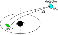
Figure 2: Denomination of various elements of solid angles and areas defined in the text: a) the light source appears to the observer to be point-like; b) the light rays received by the detector are coming from different parts of the disc (closer view of the disc than in previous figure); c) area of a light tube changes as the light rays travel close to the black hole (the disc is edge on).

The emission arriving at the detector within the solid angle ${{\rm d}\Omega}$ (see Figure 2b) originates from the proper area ${\rm d}S_{{\rm l}}$ on the disc (as measured in the rest frame co-moving with the disc). Hence, in our computations we want to integrate the flux contributions over a fine mesh on the disc surface. To achieve this aim, we adjust eq. (1) to the form

$$N^{S}_{\rm o}(E)=\frac{1}{D^{2}}\int{\rm d}S\,\frac{D^{2}{\rm d}\Omega}{{\rm d}S}\,N_{{\rm l}}(E/g)\,g^{2}=\frac{1}{D^{2}}\int{\rm d}S\,\frac{{\rm d}S_{\perp}}{{\rm d}S}\,\frac{{\rm d}S_{\rm f}}{{\rm d}S_{\perp}}\,N_{{\rm l}}(E/g)\,g^{2}\,.$$ (3)

Here ${{\rm{}d}S_{\rm f}}$ stands for an element of area perpendicular to light rays corresponding to the solid angle ${\rm d}\Omega$ at a distance $D$, ${{\rm{}d}S_{\perp}}$ is the proper area measured in the local frame of the disc and perpendicular to the rays, and ${\rm d}S$ is the coordinate area for integration. We integrate in a two-dimensional slice of a four-dimensional space-time, which is specified by coordinates $\theta=\pi/2$ and $t=t_{\rm o}-\Delta t$ with $\Delta t$ being a time delay with which photons from different parts of the disc (that lies in the equatorial plane) arrive to the observer (at the same coordinate time $t_{\rm o}$). Therefore, let us define the coordinate area by (we employ coordinates $t^{\prime},\,\theta,\,r,\,\varphi$ with $t^{\prime}=t-\Delta t$ and $\Delta t=\Delta t(r,\theta,\varphi)$)

$${\rm d}S\equiv|{\rm d}^{2}{\!S_{t^{\prime}}}^{\theta}|=\left|\frac{\partial x^{\mu}}{\partial t^{\prime}}{\rm d}^{2}{\!S_{\mu}}^{\theta}\right|=|{\rm d}^{2}{\!S_{t}}^{\theta}|=|g^{\theta\mu}{\rm d}^{2}\!S_{t\mu}|\,.$$ (4)

We define the tensor ${\rm d}^{2}\!S_{\alpha\beta}$ by two four-vector elements ${\rm d}x_{1}^{\mu}\equiv({\rm d}t_{1},{\rm d}r,0,0)$ and ${\rm d}x_{2}^{\mu}\equiv({\rm d}t_{2},0,0,{\rm d}\varphi)$ and by Levi-Civita tensor $\varepsilon_{\alpha\beta\gamma\delta}$. The time components of these vectors, ${\rm d}t_{1}$ and ${\rm d}t_{2}$, are such that the vectors ${\rm d}x_{1}^{\mu}$ and ${\rm d}x_{2}^{\mu}$ lie in the tangent space to the above defined space-time slice. Then we obtain

$${\rm d}S=|g^{\theta\theta}\varepsilon_{t\theta\alpha\beta}\,{\rm d}x_{1}^{[\alpha}{\rm d}x_{2}^{\beta]}|=g^{\theta\theta}\sqrt{-\|g_{\mu\nu}\|}\,{\rm d}r\,{\rm d}\varphi={\rm d}r\,{\rm d}\varphi\,,$$ (5)

where $g_{\mu\nu}$ is the metric tensor and $\|g_{\mu\nu}\|$ is the determinant of the metric. The proper area, ${\rm d}S_{\perp}$, perpendicular to the light ray can be expressed covariantly in the following way:

$${\rm d}S_{\perp}=-\frac{U^{\alpha}\,p^{\beta}\,{\rm d}^{2}\!S_{\alpha\beta}}{U^{\mu}\,p_{\mu}}\,.$$ (6)

Here, ${\rm d}S_{\perp}$ is the projection of an element of area, defined by ${\rm d}^{2}\!S_{\alpha\beta}$, on a spatial slice of an observer with velocity $U^{\alpha}$ and perpendicular to light rays. $U^{\alpha}$ is four-velocity of an observer measuring the area ${\rm d}S_{\perp}$, and $p^{\beta}$ is four-momentum of the photon. The proper area ${\rm d}S_{\perp}$ corresponding to the same flux tube is identical for all observers. This means that the last equation holds true for any four-velocity $U^{\alpha}$, and we can express it as

$$p^{\beta}\,{\rm d}^{2}\!S_{\alpha\beta}+p_{\alpha}\,{\rm d}S_{\perp}=0,\quad\alpha=t,r,\theta,\varphi.$$ (7)

For $\alpha=t$ (note that ${\rm d}^{2}\!S_{tr}={\rm d}^{2}\!S_{t\varphi}=0$) we get

$$\frac{{\rm d}S_{\perp}}{{\rm d}S}=\left|\frac{1}{g^{\theta\theta}}\frac{{\rm d}S_{\perp}}{{\rm d}^{2}\!S_{t\theta}}\right|=\left|-\frac{p_{\theta}}{p_{t}}\right|=\frac{r\mu_{\rm e}}{g}\,.$$ (8)

In the last equation we used the formula for the cosine of local emission angle $\mu_{\rm e}$, see eq. (A67), and the fact that we have chosen such an affine parameter of the light geodesic that $p_{t}=-1$. From eqs. (3), (4) and (8) we get for the observed flux per unit solid angle

$$N^{\Omega}_{\rm o}(E)\equiv\frac{{\rm d}n(E)}{{\rm d}t\,{\rm d}\Omega_{\rm o}}={N_{0}}\int_{r_{\rm in}}^{r_{\rm out}}{\rm d}r\,\int_{\phi}^{\phi+{\Delta\phi}}{\rm d}\varphi\,N_{{\rm l}}(E/g)\,g\,l\,\mu_{\rm e}\,r,$$ (9)

where $N_{0}$ is a normalization constant and

$$l=\frac{{\rm d}S_{\rm f}}{{\rm d}S_{\perp}}$$ (10)

is the lensing factor in the limit $D\rightarrow\infty$ (the limit is performed while keeping $D^{2}{\rm d}\Omega$ constant, see Figure 2c).

For the line emission, the normalization constant $N_{0}$ is chosen in such a way that the total flux from the disc is unity. In the case of a continuum model, the flux is normalized to unity at a certain value of the observed energy (typically at $E=1$ keV, as in other xspec models).

Finally, the integrated flux per energy bin, $\Delta E$, is

$${\Delta}N^{\Omega}_{\rm o}(E,\Delta E,t) = \int_{E}^{E+\Delta E}{\rm d}\bar{E}\,N^{\Omega}_{\rm o}(\bar{E},t)=$$ (11)

$$= N_{0}\int_{r_{\rm in}}^{r_{\rm out}}\!\!{\rm d}r\,\int_{\phi}^{\phi+{\Delta\phi}}\!\!{\rm d}\varphi\,\int_{E/g}^{(E+\Delta E)/g}\!\!{\rm d}E_{{\rm l}}\,N_{{\rm l}}(E_{{\rm l}},r,\varphi,\mu_{\rm e},t-\Delta t)\,g^{2}\,l\,\mu_{\rm e}\,r\,,\hskip 5.69054pt$$

where $\Delta t$ is the relative time delay with which photons arrive to the observer from different parts of the disc. The transfer functions $g,\,l,\,\mu_{\rm e}$ and $\Delta t$ are read from the FITS file KBHtablesNN.fits described in Appendix A.3.1. This equation is numerically integrated for a given local flux $N_{\rm l}(E_{{\rm l}},r,\varphi,\mu_{\rm e},t-\Delta t)$ in all hereby described new general relativistic non-axisymmetric models.

Let us assume that the local emission is stationary and the dependence on the axial coordinate is only through the prescribed dependence on the local emission angle $f(\mu_{\rm e})$ (limb darkening/brightening law) together with an arbitrary radial dependence $R(r)$, i.e.

$$N_{\rm l}(E_{{\rm l}},r,\varphi,\mu_{\rm e},t-\Delta t)\equiv N_{\rm l}(E_{\rm l})\,R(r)\,f(\mu_{\rm e}).$$ (12)

The observed flux $N_{\rm o}^{\Omega}(E)$ is in this case given by

$$N_{\rm o}^{\Omega}(E)=\int_{-\infty}^{\infty}{\rm d}E_{\rm l}\,N_{\rm l}(E_{\rm l})\,G(E,E_{\rm l}),$$ (13)

where

$$G(E,E_{\rm l})=N_{0}\int_{r_{\rm in}}^{r_{\rm out}}{\rm d}r\,R(r)\int_{0}^{2\pi}{\rm d}\varphi\,f(\mu_{\rm e})\,g^{2}\,l\,\mu_{\rm e}\,r\,\delta(E-gE_{\rm l}).$$ (14)

In this case, the integrated flux can be expressed in the following way:

$${\Delta}N^{\Omega}_{\rm o}(E,\Delta E) = \int_{E}^{E+\Delta E}{\rm d}\bar{E}\,N^{\Omega}_{\rm o}(\bar{E})\quad=\hskip 199.16928pt$$ (15)

$$=\int_{E}^{E+\Delta E}{\rm d}\bar{E}\,{N_{0}}\int_{r_{\rm in}}^{r_{\rm out}}{\rm d}r\,R(r)\,\int_{0}^{2\pi}{\rm d}\varphi\,f(\mu_{\rm e})\,N_{{\rm l}}(\bar{E}/g)\,g\,l\,\mu_{\rm e}\,r\,\int_{-\infty}^{\infty}{\rm d}E_{\rm l}\,\delta(E_{\rm l}-\bar{E}/g)=$$

$$=N_{0}\int_{r_{\rm in}}^{r_{\rm out}}{\rm d}r\,R(r)\,\int_{-\infty}^{\infty}{\rm d}E_{{\rm l}}\,N_{{\rm l}}(E_{{\rm l}})\int_{E/E_{{\rm l}}}^{(E+\Delta E)/E_{{\rm l}}}{\rm d}\bar{g}\,F(\bar{g})\,,$$

where we substituted $\bar{g}=\bar{E}/E_{\rm l}$ and

$$F(\bar{g})=\int_{0}^{2\pi}{\rm d}\varphi\,f(\mu_{\rm e})\,g^{2}\,l\,\mu_{\rm e}\,r\,\delta(\bar{g}-g)\,.$$ (16)

Eq. (15) is numerically integrated in all axially symmetric models. The function ${\rm d}F(\bar{g})\equiv{\rm d}\bar{g}\,F(\bar{g})$ has been pre-calculated for several limb darkening/brightening laws $f(\mu_{\rm e})$ and stored in separate files, KBHlineNN.fits (see Appendix A.3.2).

4 Stokes parameters in strong gravity regime

For polarization studies, Stokes parameters are used. Let us define specific Stokes parameters in the following way:

$$i_{\nu}\equiv\frac{I_{\nu}}{E}\,,\quad q_{\nu}\equiv\frac{Q_{\nu}}{E}\,,\quad u_{\nu}\equiv\frac{U_{\nu}}{E}\,,\quad v_{\nu}\equiv\frac{V_{\nu}}{E}\,,$$ (17)

where $I_{\nu}$, $Q_{\nu}$, $U_{\nu}$ and $V_{\nu}$ are Stokes parameters for light with frequency $\nu$, $E$ is energy of a photon at this frequency. Further on, we drop the index $\nu$ but we will always consider these quantities for light of a given frequency. We can calculate the integrated specific Stokes parameters (per energy bin), i.e. $\Delta i_{\rm o}$, $\Delta q_{\rm o}$, $\Delta u_{\rm o}$ and $\Delta v_{\rm o}$. These are the quantities that the observer determines from the local specific Stokes parameters $i_{\rm l}$, $q_{\rm l}$, $u_{\rm l}$ and $v_{\rm l}$ on the disc in the following way:

$${\Delta}i_{\rm o}(E,\Delta E) = N_{0}\int{\rm d}S\,\int{\rm d}E_{{\rm l}}\,i_{{\rm l}}(E_{{\rm l}})\,Fr\,,$$ (18)

$${\Delta}q_{\rm o}(E,\Delta E) = N_{0}\int{\rm d}S\,\int{\rm d}E_{{\rm l}}\,[q_{{\rm l}}(E_{{\rm l}})\cos{2\Psi}-u_{{\rm l}}(E_{{\rm l}})\sin{2\Psi}]\,Fr\,,$$ (19)

$${\Delta}u_{\rm o}(E,\Delta E) = N_{0}\int{\rm d}S\,\int{\rm d}E_{{\rm l}}\,[q_{{\rm l}}(E_{{\rm l}})\sin{2\Psi}+u_{{\rm l}}(E_{{\rm l}})\cos{2\Psi}]\,Fr\,,$$ (20)

$${\Delta}v_{\rm o}(E,\Delta E) = N_{0}\int{\rm d}S\,\int{\rm d}E_{{\rm l}}\,v_{{\rm l}}(E_{{\rm l}})\,Fr\,.$$ (21)

Here, $F\equiv F(r,\varphi)=g^{2}\,l\,\mu_{\rm e}$ is a transfer function, $\Psi$ is the angle by which a vector parallelly transported along the light geodesic rotates. We refer to this angle also as a change of the polarization angle, because the polarization vector is parallelly transported along light geodesics. See Figure 3 for an exact definition of the angle $\Psi$. The integration boundaries are the same as in eq. (11). As can be seen from the definition, the first specific Stokes parameter is equal to the photon flux, therefore, eqs. (11) and (18) are identical. The local specific Stokes parameters may depend on $r$, $\varphi$, $\mu_{\rm e}$ and $t-\Delta t$, which we did not state in the eqs. (18)–(21) explicitly for simplicity.

The specific Stokes parameters that the observer measures may vary in time in the case when the local parameters also depend on time. In eqs. (18)–(21) we used a law of transformation of the Stokes parameters by the rotation of axes (eqs. (I.185) and (I.186) in [4]).

(i) Let three-vectors $p_{A}$, $n_{A}$, $n^{\prime}_{A}$ and $f_{A}$ be the momentum of a photon, normal to the disc, projection of the normal to the plane perpendicular to the momentum and a vector which is parallelly transported along the geodesic (as four-vector), respectively; (ii) let $\Psi_{A}$ be an angle between $n^{\prime}_{A}$ and $f_{A}$; (iii) let the quantities in (i) and (ii) be evaluated at the disc for $A=1$ with respect to the local rest frame co-moving with the disc, and at infinity for $A=2$ with respect to the stationary observer at the same light geodesic; (iv) then the change of polarization angle is defined as $\Psi=\Psi_{2}-\Psi_{1}$.

Figure 3: Definition of the change of polarization angle $\Psi$.

An alternative way for expressing polarization of light is by using the degree of polarization $P_{\rm o}$ and two polarization angles $\chi_{\rm o}$ and $\xi_{\rm o}$, defined by

$$P_{\rm o} = \sqrt{q_{\rm o}^{2}+u_{\rm o}^{2}+v_{\rm o}^{2}}/i_{\rm o}\,,$$ (22)

$$\tan{2\chi_{\rm o}} = u_{\rm o}/q_{\rm o}\,,$$ (23)

$$\sin{2\xi_{\rm o}} = v_{\rm o}/\sqrt{q_{\rm o}^{2}+u_{\rm o}^{2}+v_{\rm o}^{2}}\,.$$ (24)

5 New model for xspec

We have developed several general relativistic models for line emission and Compton reflection continuum. The line models are supposed to be more accurate and versatile than the laor model [19], and substantially faster than the kerrspec model [20]. Several models of intrinsic emissivity were employed, including the lamp-post model [22]. Among other features, these models allow various parameters to be fitted such as the black-hole angular momentum, observer inclination, accretion disc size and some of the parameters characterizing disc emissivity and primary illumination properties. They also allow a change in the grid resolution and, hence, to control accuracy and computational speed. Furthermore, we developed very general convolution models. All these models are based on pre-calculated tables described in Section 2 and thus the geodesics do not need to be calculated each time one integrates the disc emission. These tables are calculated for the vacuum Kerr space-time and for a Keplerian co-rotating disc plus matter that is freely falling below the marginally stable orbit. The falling matter has the energy and angular momentum of the matter at the marginally stable orbit. It is possible to use different pre-calculated tables if they are stored in a specific FITS file (see Appendix A.3.1 for its detailed description).

There are two types of new models. The first type integrates the local disc emission in both of the polar coordinates on the disc and thus enables one to choose non-axisymmetric area of integration. This option is useful for example when computing spectra of spots or partially obscured discs. One can also choose the resolution of integration and thus control the precision and speed of the computation. The second type of models is axisymmetric – the axially dependent part of the emission from rings is pre-calculated and stored in a FITS file (the function ${\rm d}F(\bar{g})={\rm d}\bar{g}\,F(\bar{g})$ from (16) is integrated for different radii with the angular grid having $20\,000$ points). These models have less parameters that can be fitted and thus are less flexible even though more suited to the standard analysis approach. On the other hand they are fast because the emission is integrated only in one dimension (in the radial coordinate of the disc). It may be worth emphasizing that the assumption about axial symmetry concerns only the form of intrinsic emissivity of the disc, which cannot depend on the polar angle in this case, not the shape of individual light rays, which is always complicated near a rotating black hole.

parameter	unit	default value	minimum value	maximum value
a/M	$GM/c$	0.9982	0.	1.
theta_o	deg	30.	0.	89.
rin-rh	$GM/c^{2}$	0.	0.	999.
ms	–	1.	0.	1.
rout-rh	$GM/c^{2}$	400.	0.	999.
zshift	–	0.	-0.999.	10.
ntable	–	0.	0.	99.

Table 1: Common parameters for all models.

There are several parameters and switches that are common for all new models (see Table 1):

a/M

– specific angular momentum of the Kerr black hole in units of $GM/c$ ($M$ is the mass of the central black hole),

theta_o

– the inclination of the observer in degrees,

rin-rh

– inner radius of the disc relative to the black-hole horizon in units of $GM/c^{2}$,

ms

– switch for the marginally stable orbit,

rout-rh

– outer radius of the disc relative to the black-hole horizon in units of $GM/c^{2}$,

zshift

– overall redshift of the object,

ntable

– number of the FITS file with pre-calculated tables to be used.

The inner and outer radii are given relative to the black-hole horizon and, therefore, their minimum value is zero. This becomes handy when one fits the a/M parameter, because the horizon of the black hole as well as the marginally stable orbit changes with a/M, and so the lower limit for inner and outer disc edges cannot be set to constant values. The ms switch determines whether we intend to integrate also emission below the marginally stable orbit. If its value is set to zero and the inner radius of the disc is below this orbit then the emission below the marginally stable orbit is taken into account, otherwise it is not.

The ntable switch determines which of the pre-calculated tables should be used for intrinsic emissivity. In particular, ${\tt ntable}=0$ for KBHtables00.fits (KBHline00.fits), ${\tt ntable}=1$ for KBHtables01.fits (KBHline01.fits), etc., corresponding to non-axisymmetric (axisymmetric) models.

parameter	unit	default value	minimum value	maximum value
phi	deg	0.	-180.	180.
dphi	deg	360.	0.	360.
nrad	–	200.	1.	10000.
division	–	1.	0.	1.
nphi	–	180.	1.	20000.
smooth	–	1.	0.	1.
Stokes	–	0.	0.	6.

Table 2: Common parameters for non-axisymmetric models.

The following set of parameters is relevant only for non-axisymmetric models (see Table 2):

phi

– position angle of the axial sector of the disc in degrees,

dphi

– inner angle of the axial sector of the disc in degrees,

nrad

– radial resolution of the grid,

division

– switch for spacing of radial grid ($0$ – equidistant, $1$ – exponential),

nphi

– axial resolution of the grid,

smooth

– switch for performing simple smoothing ($0$ – no, $1$ – yes),

Stokes

– switch for computing polarization (see Table 3).

The phi and dphi parameters determine the axial sector of the disc from which emission comes (see Figure 4). The nrad and nphi parameters determine the grid for numerical integration. If the division switch is zero, the radial grid is equidistant; if it is equal to unity then the radial grid is exponential (i.e. more points closer to the black hole).

If the smooth switch is set to unity then a simple smoothing is applied to the final spectrum. Here $N_{\rm o}^{\Omega}(E_{{\rm l}})=[N_{\rm o}^{\Omega}(E_{\rm i-1})+2N_{\rm o}^{\Omega}(E_{{\rm l}})+N_{\rm o}^{\Omega}(E_{\rm i+1})]/4$.

If the Stokes switch is different from zero, then the model also calculates polarization. Its value determines, which of the Stokes parameters should be computed by xspec, i.e. what will be stored in the output array for the photon flux photar; see Table 3. (If ${\tt Stokes}\neq 0$ then a new ascii data file stokes.dat is created in the current directory, where values of energy $E$ together with all Stokes parameters $i,\,q,\,u,\,v,\,P,\,\chi$[deg] and $\xi$[deg] are stored, each in one column.)

A realistic model of polarization has been currently implemented only in the kyl1cr model (see Section 7.1 below). In other models, a simple assumption is made – the local emission is assumed to be linearly polarized in the direction perpendicular to the disc (i.e. $q_{{\rm l}}=i_{{\rm l}}=N_{\rm l}$ and $u_{\rm l}=v_{\rm l}=0$). In all models (including kyl1cr) there is always no final circular polarization (i.e. $v=\xi=0$), which follows from the fact that the fourth local Stokes parameter is zero in each model.

Figure 4: Segment of a disc from which emission comes (view from above).

value	photon flux array photar contains${}^{{\dagger}}{}^{{\ddagger}}$
0	$i=I/E$, where $I$ is the first Stokes parameter (intensity)
1	$q=Q/E$, where $Q$ is the second Stokes parameter
2	$u=U/E$, where $U$ is the third Stokes parameter
3	$v=V/E$, where $V$ is the fourth Stokes parameter
4	degree of polarization, $P=\sqrt{q^{2}+u^{2}+v^{2}}/i$
5	angle $\chi$[deg] of polarization, $\tan{2\chi}=u/q$
6	angle $\xi$[deg] of polarization, $\sin{2\xi}=v/\sqrt{q^{2}+u^{2}+v^{2}}$
† the photar array contains values described in the table and multiplied by width of the corresponding energy bin ${}^{{\ddagger}}~{}E$ is energy of observed photons

Table 3: Definition of the Stokes parameter.

6 Models for a relativistic spectral line

Three general relativistic line models are included in the new set of xspec routines – non-axisymmetric Gaussian line model kyg1line, axisymmetric Gaussian line model kygline and fluorescent lamp-post line model kyf1ll.

6.1 Non-axisymmetric Gaussian line model kyg1line

The kyg1line model computes the integrated flux from the disc according to eq. (11). It assumes that the local emission from the disc is

$$N_{{\rm l}}(E_{\rm l}) = \frac{1}{r^{\tt alpha}}\,f(\mu_{\rm e})\,\exp{\left[-\left(1000\,\frac{E_{\rm l}-{\tt Erest}}{\sqrt{2}\,{\tt sigma}}\right)^{2}\right]}\quad{\rm for}\quad r\geq r_{\rm b}\,,$$ (25)

$$N_{{\rm l}}(E_{\rm l}) = {\tt jump}\ r_{\rm b}^{{\tt beta}-{\tt alpha}}\,\frac{1}{r^{\tt beta}}\,f(\mu_{\rm e})\,\exp{\left[-\left(1000\,\frac{E_{\rm l}-{\tt Erest}}{\sqrt{2}\,{\tt sigma}}\right)^{2}\right]}\quad{\rm for}\quad r<r_{\rm b}\,.\hskip 14.22636pt$$ (26)

The local emission is assumed to be a Gaussian line with its peak flux depending on the radius as a broken power law. The line is defined by nine points equally spaced with the central point at its maximum. The normalization constant $N_{0}$ in (11) is such that the total integrated flux of the line is unity. The parameters defining the Gaussian line are (see Table 4):

Erest

– rest energy of the line in keV,

sigma

– width of the line in eV,

alpha

– radial power-law index for the outer region,

beta

– radial power-law index for the inner region,

rb

– parameter defining the border between regions with different power-law indices,

jump

– ratio between flux in the inner and outer regions at the border radius,

limb

– switch for different limb darkening/brightening laws.

There are two regions with different power-law dependences with indices alpha and beta. The power law changes at the border radius $r_{\rm b}$ where the local emissivity does not need to be continuous (for ${\tt jump}\neq 1$). The rb parameter defines this radius in the following way:

$$r_{\rm b} = {\tt rb}\times r_{\rm ms}\quad{\rm for}\quad{\tt rb}\geq 0\,,$$ (27)

$$r_{\rm b} = -{\tt rb}+r_{\rm h}\quad{\rm for}\quad{\tt rb}<0\,,$$ (28)

where $r_{\rm ms}$ is the radius of the marginally stable orbit and $r_{\rm h}$ is the radius of the horizon of the black hole.

parameter		unit	default value	minimum value	maximum value
	a/M	$GM/c$	0.9982	0.	1.
	theta_o	deg	30.	0.	89.
	rin-rh	$GM/c^{2}$	0.	0.	999.
	ms	–	1.	0.	1.
	rout-rh	$GM/c^{2}$	400.	0.	999.
	phi	deg	0.	-180.	180.
	dphi	deg	360.	0.	360.
	nrad	–	200.	1.	10000.
	division	–	1.	0.	1.
	nphi	–	180.	1.	20000.
	smooth	–	1.	0.	1.
	zshift	–	0.	-0.999	10.
	ntable	–	0.	0.	99.
*	Erest	keV	6.4	1.	99.
*	sigma	eV	2.	0.01	1000.
*	alpha	–	3.	-20.	20.
*	beta	–	4.	-20.	20.
*	rb	$r_{\rm ms}$	0.	0.	160.
*	jump	–	1.	0.	1e6
*	limb	–	-1.	-10.	10.
	Stokes	–	0.	0.	6.

Table 4: Parameters of the non-axisymmetric Gaussian line model kyg1line. Model parameters that are not common for all non-axisymmetric models are denoted by asterisk.

The function $f(\mu_{\rm e})=f(\cos{\,\delta_{\rm e}})$ in (25) and (26) describes the limb darkening/brightening law, i.e. the dependence of the local emission on the local emission angle. Several limb darkening/brightening laws are implemented:

$$f(\mu_{\rm e}) = 1\quad{\rm for}\quad{\tt limb}=0\,,$$ (29)

$$f(\mu_{\rm e}) = 1+2.06\mu_{\rm e}\quad{\rm for}\quad{\tt limb}=-1\,,$$ (30)

$$f(\mu_{\rm e}) = \ln{(1+\mu_{\rm e}^{-1})}\quad{\rm for}\quad{\tt limb}=-2\,,$$ (31)

$$f(\mu_{\rm e}) = \mu_{\rm e}^{\tt limb}\quad{\rm for}\quad{\tt limb}\neq 0,-1,-2\,.$$ (32)

Eq. (29) corresponds to the isotropic local emission, eq. (30) corresponds to limb darkening in an optically thick electron scattering atmosphere (used by Laor [18, 19, 25]), and eq. (31) corresponds to limb brightening predicted by some models of a fluorescent line emitted by an accretion disc due to X-ray illumination [13, 15].

There is also a similar model kyg2line present among the new xspec models, which is useful when fitting two general relativistic lines simultaneously. The parameters are the same as in the kyg1line model except that there are two sets of those parameters describing the local Gaussian line emission. There is one more parameter present, ratio21, which is the ratio of the maximum of the second local line to the maximum of the first local line. Polarization computations are not included in this model.

6.2 Axisymmetric Gaussian line model kygline

This model uses eq. (15) for computing the disc emission with local flux being

$$N_{\rm l}(E_{\rm l}) = \delta(E_{\rm l}-{\tt Erest})\,,$$ (33)

$$R(r) = r^{-{\tt alpha}}\,.$$ (34)

The function ${\rm d}F(\bar{g})\equiv{\rm d}\bar{g}\,F(\bar{g})$ in (16) was pre-calculated for three different limb darkening/brightening laws (29) – (31) and stored in corresponding FITS files KBHline00.fits – KBHline02.fits. The local emission is a delta function with its maximum depending on the radius as a power law with index alpha and also depending on the local emission angle. The normalization constant $N_{0}$ in (15) is such that the total integrated flux of the line is unity.

parameter		unit	default value	minimum value	maximum value
	a/M	$GM/c$	0.9982	0.	1.
	theta_o	deg	30.	0.	89.
	rin-rh	$GM/c^{2}$	0.	0.	999.
	ms	–	1.	0.	1.
	rout-rh	$GM/c^{2}$	400.	0.	999.
	zshift	–	0.	-0.999	10.
	ntable	–	1.	0.	99.
*	Erest	keV	6.4	1.	99.
*	alpha	–	3.	-20.	20.

Table 5: Parameters of the axisymmetric Gaussian line model kygline. Model parameters that are not common for all axisymmetric models are denoted by asterisk.

There are less parameters defining the line in this model than in the previous one (see Table 5):

Erest

– rest energy of the line in keV,

alpha

– radial power-law index.

Note that the limb darkening/brightening law can be chosen by means of the ntable switch.

This model is much faster than the non-axisymmetric kyg1line model. Although it is not possible to change the resolution grid on the disc, it is hardly needed because the resolution is set to be very large, corresponding to ${\tt nrad}=500$, ${\tt division}=1$ and ${\tt nphi}=20\,000$ in the kyg1line model, which is more than sufficient in most cases. (These values apply if the maximum range of radii is selected, i.e. rin=0, ms=0 and rout=999; in case of a smaller range the number of points decreases accordingly.) This means that the resolution of the kyg1line model is much higher than what can be achieved with the laor model, and the performance is still very good.

6.3 Non-axisymmetric fluorescent lamp-post line model kyf1ll

The line in this model is induced by the illumination of the disc from the primary power-law source located on the axis at height above the black hole. This model computes the final spectrum according to eq. (11) with the local photon flux

$$N_{{\rm l}}(E_{\rm l}) = g_{\rm L}^{{\tt PhoIndex}-1}\frac{\sin\theta_{\rm L}{\rm d}\theta_{\rm L}}{r\,{\rm d}r}\,\sqrt{1-\frac{2{\tt height}}{{\tt height}^{2}+a^{2}}}\,f(\mu_{\rm i},\mu_{\rm e})$$ (35)

$$\times\ \exp{\left[-\left(1000\,\frac{E_{\rm l}-{\tt Erest}}{\sqrt{2}\,{\tt sigma}}\right)^{2}\right]}.$$

Here, $g_{\rm L}$ is ratio of the energy of a photon received by the accretion disc to the energy of the same photon when emitted from a source on the axis, $\theta_{\rm L}$ is an angle under which the photon is emitted from the source (measured in the local frame of the source) and $\mu_{\rm i}\equiv\cos{\,\delta_{\rm i}}$ is the cosine of the incident angle (measured in the local frame of the disc) – see Figure 5. All of these functions depend on height above the black hole at which the source is located and on the rotational parameter a/M of the black hole. Values of $g_{\rm L}$, $\theta_{\rm L}$ and $\mu_{\rm i}$ for a given height and rotation are read from the lamp-post tables lamp.fits (see Appendix A.3.3). At present, only tables for ${\tt a/M}=0.9987492$ (i.e. for the horizon of the black hole $r_{\rm h}=1.05$) and ${\tt height}=$ $2$,$\,3,\,4,\,5,\,6,\,8,\,10,\,12$,$\,15,\,20,\,30,\,50,\,75$ and $100$ are included in lamp.fits, therefore, the a/M parameter is used only for the negative values of height (see below).

The factor in front of the function $f(\mu_{\rm i},\mu_{\rm e})$ gives the radial dependence of the disc emissivity, which is different from the assumed broken power law in the kyg1line model. For the derivation of this factor, which characterizes the illumination from a primary source on the axis see Appendix A.2.

parameter		unit	default value	minimum value	maximum value
	a/M	$GM/c$	0.9982	0.	1.
	theta_o	deg	30.	0.	89.
	rin-rh	$GM/c^{2}$	0.	0.	999.
	ms	–	1.	0.	1.
	rout-rh	$GM/c^{2}$	400.	0.	999.
	phi	deg	0.	-180.	180.
	dphi	deg	360.	0.	360.
	nrad	–	200.	1.	10000.
	division	–	1.	0.	1.
	nphi	–	180.	1.	20000.
	smooth	–	1.	0.	1.
	zshift	–	0.	-0.999	10.
	ntable	–	0.	0.	99.
*	PhoIndex	–	2.	1.5	3.
*	height	$GM/c^{2}$	3.	-20.	100.
*	Erest	keV	6.4	1.	99.
*	sigma	eV	2.	0.01	1000.
	Stokes	–	0.	0.	6.

Table 6: Parameters of the fluorescent lamp-post line model kyf1ll. Model parameters that are not common for all non-axisymmetric models are denoted by asterisk.

The function $f(\mu_{\rm i},\mu_{\rm e})$ is a coefficient of reflection. It depends on the incident and reflection angles. Although the normalization of this function also depends on the photon index of the power-law emission from a primary source, we do not need to take this into account because the final spectrum is always normalized to unity. Values of this function are read from a pre-calculated table which is stored in fluorescent_line.fits file (see [21] and Appendix A.3.4).

The local emission (35) is defined in nine points of local energy $E_{\rm l}$ that are equally spaced with the central point at its maximum. The normalization constant $N_{0}$ in the formula (11) is such that the total integrated flux of the line is unity. The parameters defining local emission in this model are (see Table 6):

PhoIndex

– photon index of primary power-law illumination,

height

– height above the black hole where the primary source is located for ${\tt height}>0$, and radial power-law index for ${\tt height}\leq 0$,

Erest

– rest energy of the line in keV,

sigma

– width of the line in eV.

If positive, the height parameter works as a switch – the exact value present in the tables lamp.fits must be chosen. If the height parameter is negative, then this model assumes that the local emission is the same as in the kyg1line model with the parameters ${\tt alpha}=-{\tt height}$, ${\tt rb=0}$ and ${\tt limb}=-2$ (PhoIndex parameter is unused in this case).

a)	b)

Figure 5: Reflection models: a) lamp-post model; b) diffuse corona model.

7 Compton reflection models

We have developed two new relativistic continuum models – lamp-post Compton reflection model kyl1cr and the kyh1refl model which is a relativistically blurred hrefl model that is already present in xspec. Both of these models are non-axisymmetric.

7.1 Non-axisymmetric lamp-post Compton reflection model kyl1cr

The emission in this model is induced by the illumination of the disc from the primary power-law source located on the axis at height above the black hole. As in every non-axisymmetric model the observed spectrum is computed according to eq. (11). The local emission is

$$N_{{\rm l}}(E_{\rm l}) = g_{\rm L}^{{\tt PhoIndex}-1}\frac{\sin\theta_{\rm L}{\rm d}\theta_{\rm L}}{r\,{\rm d}r}\,\sqrt{1-\frac{2{\tt height}}{{\tt height}^{2}+({\tt a/M})^{2}}}\,f(E_{\rm l};\mu_{\rm i},\mu_{\rm e})\quad{\rm for}\quad{\tt height}>0\,,\hskip 10.00002pt$$ (36)

$$N_{{\rm l}}(E_{\rm l}) = r^{\tt height}\,\bar{f}(E_{\rm l};\mu_{\rm e})\quad{\rm for}\quad{\tt height\leq 0}\,.$$ (37)

For the definition of $g_{\rm L}$, $\theta_{\rm L}$ and $\mu_{\rm i}$ see Section 6.3 and Appendix A.3.3, where pre-calculated tables of these functions in lamp.fits are described.

The function $f(E_{\rm l};\mu_{\rm i},\mu_{\rm e})$ gives dependence of the locally emitted spectrum on the angle of incidence and the angle of emission, assuming a power-law illumination. This function depends on the photon index PhoIndex of the power-law emission from a primary source. Values of this function for various photon indices of primary emission are read from the pre-calculated tables stored in refspectra.fits (see Appendix A.3.5). These tables were calculated by the Monte Carlo simulations of Compton scattering [21]. At present, tables for ${\tt PhoIndex}=1.5,\ 1.6,\ \dots,\ 2.9,\ 3.0$ and for local energies in the range from $2$ keV to $300$ keV are available. The normalization constant $N_{0}$ in eq. (11) is such that the final photon flux at an energy of $3$ keV is equal to unity, which is different from what is usual for continuum models in xspec (where the photon flux is unity at $1$ keV). The choice adopted is due to the fact that current tables in refspectra.fits do not extend below $2$ keV.

The function $\bar{f}(E_{\rm l};\mu_{\rm e})$, which is used for negative height, is an averaged function $f(E_{\rm l};\mu_{\rm i},\mu_{\rm e})$ over $\mu_{\rm i}$

$$\bar{f}(E_{\rm l};\mu_{\rm e})\equiv\int_{0}^{1}{\rm d}\mu_{\rm i}\,f(E_{\rm l};\mu_{\rm i},\mu_{\rm e})\,.$$ (38)

The local emission (37) can be interpreted as emission induced by illumination from clouds localized near above the disc rather than from a primary source on the axis (see Figure 5). In this case photons strike the disc from all directions.

For positive values of height the kyl1cr model includes a physical model of polarization based on Rayleigh scattering in single scattering approximation. The specific local Stokes parameters describing local polarization of light are

$$i_{\rm l}(E_{\rm l}) = \frac{I_{\rm l}+I_{\rm r}}{\langle I_{\rm l}+I_{\rm r}\rangle}\,N_{\rm l}(E_{\rm l})\,,$$ (39)

$$q_{\rm l}(E_{\rm l}) = \frac{I_{\rm l}-I_{\rm r}}{\langle I_{\rm l}+I_{\rm r}\rangle}\,N_{\rm l}(E_{\rm l})\,,$$ (40)

$$u_{\rm l}(E_{\rm l}) = \frac{U}{\langle I_{\rm l}+I_{\rm r}\rangle}\,N_{\rm l}(E_{\rm l})\,,$$ (41)

$$v_{\rm l}(E_{\rm l}) = 0\,,$$ (42)

where functions $I_{\rm l}$, $I_{\rm r}$ and $U$ determine the angular dependence of the Stokes parameters in the following way

$$I_{\rm l} = \mu_{\rm e}^{2}(1+\mu_{\rm i}^{2})+2(1-\mu_{\rm e}^{2})(1-\mu_{\rm i}^{2})-4\mu_{\rm e}\mu_{\rm i}\sqrt{(1-\mu_{\rm e}^{2})(1-\mu_{\rm i}^{2})}\,\cos{(\Phi_{\rm e}-\Phi_{\rm i})}$$ (43)

$$-\mu_{\rm e}^{2}(1-\mu_{\rm i}^{2})\cos{2(\Phi_{\rm e}-\Phi_{\rm i})}\,,$$

$$I_{\rm r} = 1+\mu_{\rm i}^{2}+(1-\mu_{\rm i}^{2})\cos{2(\Phi_{\rm e}-\Phi_{\rm i})}\,,$$ (44)

$$U = -4\mu_{\rm i}\sqrt{(1-\mu_{\rm e}^{2})(1-\mu_{\rm i}^{2})}\,\sin{(\Phi_{\rm e}-\Phi_{\rm i})}-2\mu_{\rm e}(1-\mu_{\rm i}^{2})\sin{2(\Phi_{\rm e}-\Phi_{\rm i})}\,,$$ (45)

Here $\Phi_{\rm e}$ and $\Phi_{\rm i}$ are the azimuthal emission and the incident angles in the local rest frame co-moving with the accretion disc (see Appendixes A.1 and A.2 for their definition). For the derivation of these formulae see the definitions (I.147) and eqs. (X.172) in [4]. We have omitted a common multiplication factor, which would be cancelled anyway in eqs. (39)–(42). The symbol $\langle\ \rangle$ in definitions of the local Stokes parameters means value averaged over the difference of the azimuthal angles $\Phi_{\rm e}-\Phi_{\rm i}$. We divide the parameters by $\langle I_{\rm l}+I_{\rm r}\rangle$ because the function $f(E_{\rm l};\mu_{\rm i},\mu_{\rm e})$, and thus also the local photon flux $N_{\rm l}(E_{\rm l})$, is averaged over the difference of the azimuthal angles.

parameter		unit	default value	minimum value	maximum value
	a/M	$GM/c$	0.9982	0.	1.
	theta_o	deg	30.	0.	89.
	rin-rh	$GM/c^{2}$	0.	0.	999.
	ms	–	1.	0.	1.
	rout-rh	$GM/c^{2}$	400.	0.	999.
	phi	deg	0.	-180.	180.
	dphi	deg	360.	0.	360.
	nrad	–	200.	1.	10000.
	division	–	1.	0.	1.
	nphi	–	180.	1.	20000.
	smooth	–	1.	0.	1.
	zshift	–	0.	-0.999	10.
	ntable	–	0.	0.	99.
*	PhoIndex	–	2.	1.5	3.
*	height	$GM/c^{2}$	3.	-20.	100.
*	line	–	0.	0.	1.
*	E_cut	keV	300.	1.	1000.
	Stokes	–	0.	0.	6.

Table 7: Parameters of the lamp-post Compton reflection model kyl1cr. Model parameters that are not common for all non-axisymmetric models are denoted by asterisk.

The parameters defining local emission in this model are (see Table 7):

PhoIndex

– photon index of primary power-law illumination,

height

– height above the black hole where the primary source is located for ${\tt height}>0$, and radial power-law index for ${\tt height}\leq 0$,

line

– switch whether to include the iron lines (0 – no, 1 – yes),

E_cut

– exponential cut-off energy of the primary source in keV.

Tables refspectra.fits for the function $f(E_{\rm l};\mu_{\rm i},\mu{\rm e})$ also contain the emission in the iron lines K$\alpha$ and K$\beta$. The two lines can be excluded from computations if the line switch is set to zero. The E_cut parameter sets the upper boundary in energies where the emission from a primary source ceases to follow a power-law dependence. If the E_cut parameter is lower than both the maximum energy of the considered dataset and the maximum energy in the tables for $f(E_{\rm l};\mu_{\rm i},\mu{\rm e})$ in refspectra.fits (300 keV), then this model is not valid.

7.2 Non-axisymmetric Compton reflection model kyh1refl

This model is based on an existing multiplicative hrefl model in combination with the powerlaw model, both of which are present in xspec. Local emission in (11) is the same as the spectrum given by the model hrefl*powerlaw with the parameters ${\tt thetamin}=0$ and ${\tt thetamax}=90$ with a broken power-law radial dependence added:

$$N_{\rm l}(E_{\rm l}) = r^{-{\tt alpha}}\,\textsc{hrefl*powerlaw}\quad{\rm for}\quad r\geq r_{\rm b}\,,$$ (46)

$$N_{\rm l}(E_{\rm l}) = {\tt jump}\,r_{\rm b}^{{\tt beta}-{\tt alpha}}\,r^{-{\tt beta}}\,\textsc{hrefl*powerlaw}\quad{\rm for}\quad r<r_{\rm b}\,.$$ (47)

For a definition of the boundary radius $r_{\rm b}$ by the rb parameter see eqs. (27)–(28), and for a detailed description of the hrefl model see [9] and the xspec manual. The kyh1refl model can be interpreted as a Compton-reflection model for which the source of primary irradiation is near above the disc, in contrast to the lamp-post scheme with the source on the axis (see Figure 5). The approximations for Compton reflection used in hrefl (and therefore also in kyh1refl) are valid below $\sim 15$ keV in the disc rest-frame. The normalization of the final spectrum in this model is the same as in other continuum models in xspec, i.e. photon flux is unity at the energy of $1$ keV.

parameter		unit	default value	minimum value	maximum value
	a/M	$GM/c$	0.9982	0.	1.
	theta_o	deg	30.	0.	89.
	rin-rh	$GM/c^{2}$	0.	0.	999.
	ms	–	1.	0.	1.
	rout-rh	$GM/c^{2}$	400.	0.	999.
	phi	deg	0.	-180.	180.
	dphi	deg	360.	0.	360.
	nrad	–	200.	1.	10000.
	division	–	1.	0.	1.
	nphi	–	180.	1.	20000.
	smooth	–	1.	0.	1.
	zshift	–	0.	-0.999	10.
	ntable	–	0.	0.	99.
*	PhoIndex	–	1.	0.	10.
*	alpha	–	3.	-20.	20.
*	beta	–	4.	-20.	20.
*	rb	$r_{\rm ms}$	0.	0.	160.
*	jump	–	1.	0.	1e6
*	Feabun	–	1.	0.	200.
*	FeKedge	keV	7.11	7.0	10.
*	Escfrac	–	1.	0.	1000.
*	covfac	–	1.	0.	1000.
	Stokes	–	0.	0.	6.

Table 8: Parameters of the reflection kyh1refl model. Model parameters that are not common for all non-axisymmetric models are denoted by asterisk.

The parameters defining the local emission in kyh1refl (see Table 8) are

PhoIndex

– photon index of the primary power-law illumination,

alpha

– radial power-law index for the outer region,

beta

– radial power-law index for the inner region,

rb

– parameter defining the border between regions with different power-law indices,

jump

– ratio between flux in the inner and outer regions at the border radius,

Feabun

– iron abundance relative to solar,

FeKedge

– iron K-edge energy,

Escfrac

– fraction of the direct flux from the power-law primary source seen by the observer,

covfac

– normalization of the reflected continuum.

8 General relativistic convolution models

We have also produced two convolution-type models, ky1conv and kyconv, which can be applied to any existing xspec model for the intrinsic X-ray emission from a disc around a Kerr black hole. We must stress that these models are substantially more powerful than the usual convolution models in xspec (these are commonly defined in terms of one-dimensional integration over energy bins). Despite the fact that our convolution models still use the standard xspec syntax in evaluating the observed spectrum (e.g. kyconv(powerlaw)), our code accomplishes a more complex operation. It still performs ray-tracing across the disc surface so that the intrinsic model contributions are integrated from different radii and azimuths on the disc.

There are several restrictions that arise from the fact that we use existing xspec models:

• by local xspec models only the energy dependence of the photon flux can be defined,

• only a certain type of radial dependence of the local photon flux can be imposed – we have chosen to use a broken power-law radial dependence,

• there is no azimuthal dependence of the local photon flux, except through limb darkening law,

• local flux depends on the binning of the data because it is defined in the centre of each bin, a large number of bins is needed for highly varying local flux.

For emissivities that cannot be defined by existing xspec models, or where the limitations mentioned above are too restrictive, one has to add a new user-defined model to xspec (by adding a new subroutine to xspec). This method is more flexible and faster than convolution models (especially when compared with the non-axisymmetric one), and hence it is recommended even for cases when these prefabricated models could be used. In any new model for xspec one can use the common ray-tracing driver for relativistic smearing of the local emission: ide for non-axisymmetric models and idre for axisymmetric ones. For a detailed description see Appendixes A.4.1 and A.4.2.

8.1 Non-axisymmetric convolution model kyc1onv

The local emission in this model is computed according to eq. (11) with the local emissivity equal to

$$N_{\rm l}(E_{\rm l}) = r^{-{\tt alpha}}\,f(\mu_{\rm e})\,\textsc{model}\quad{\rm for}\quad r>r_{\rm b}\,,$$ (48)

$$N_{\rm l}(E_{\rm l}) = {\tt jump}\,r_{\rm b}^{{\tt beta}-{\tt alpha}}\,r^{-{\tt beta}}\,f(\mu_{\rm e})\,\textsc{model}\quad{\rm for}\quad r\leq r_{\rm b}\,.\$$ (49)

For a definition of the boundary radius $r_{\rm b}$ by the rb parameter see eqs. (27)–(28) and for definition of different limb darkening laws $f(\mu_{\rm e})$ see eqs. (29)–(32). The local emission is given by the model in the centre of energy bins used in xspec with the broken power-law radial dependence and limb darkening law added. Apart from the parameters of the model, the local emission is defined also by the following parameters (see Table 9):

normal

– switch for the normalization of the final spectrum,
$=$ 0 – total flux is unity (used usually for the line),
$>$ 0 – flux is unity at the energy = normal keV (used usually for the continuum),
$<$ 0 – flux is not normalized,

ne_loc

– number of points in the energy grid where the local photon flux is defined,

alpha

– radial power-law index for the outer region,

beta

– radial power-law index for the inner region,

rb

– parameter defining the border between regions with different power-law indices,

jump

– ratio between the flux in the inner and outer regions at the border radius,

limb

– switch for different limb darkening/brightening laws.

The local emission in each ky model has to be defined either on equidistant or exponential (i.e. equidistant in logarithmic scale) energy grid. Because the energy grid used in the convolution model depends on the binning of the data, which may be arbitrary, the flux has to be rebinned. It is always rebinned into an exponentially spaced energy grid in ky convolution models. The ne_loc parameter defines the number of points in which the rebinned flux will be defined.

parameter		unit	default value	minimum value	maximum value
	a/M	$GM/c$	0.9982	0.	1.
	theta_o	deg	30.	0.	89.
	rin-rh	$GM/c^{2}$	0.	0.	999.
	ms	–	1.	0.	1.
	rout-rh	$GM/c^{2}$	400.	0.	999.
	phi	deg	0.	-180.	180.
	dphi	deg	360.	0.	360.
	nrad	–	200.	1.	10000.
	division	–	1.	0.	1.
	nphi	–	180.	1.	20000.
	smooth	–	1.	0.	1.
*	normal	–	1.	-1.	100.
	zshift	–	0.	-0.999	10.
	ntable	–	0.	0.	99.
*	ne_loc	–	100.	3.	5000.
*	alpha	–	3.	-20.	20.
*	beta	–	4.	-20.	20.
*	rb	$r_{\rm ms}$	0.	0.	160.
*	jump	–	1.	0.	1e6
*	limb	–	0.	-10.	10.
	Stokes	–	0.	0.	6.

Table 9: Parameters of the non-axisymmetric convolution model kyc1onv. Model parameters that are not common for all non-axisymmetric models are denoted by asterisk.

8.2 Axisymmetric convolution model kyconv

The local emission in this model is computed according to eq. (15) with the local emissivity equal to

$$N_{\rm l}(E_{\rm l}) = \textsc{model}\,,$$ (50)

$$R(r) = r^{-{\tt alpha}}\,.$$ (51)

Except for the parameters of the model, the local emission is defined also by the following parameters (see Table 10):

alpha

– radial power-law index,

ne_loc

– number of points in energy grid where the local photon flux is defined,

normal

– switch for the normalization of the final spectrum,
$=$ 0 – total flux is unity (used usually for the line),
$>$ 0 – flux is unity at the energy = normal keV (used usually for the continuum),
$<$ 0 – flux is not normalized.

Note that the limb darkening/brightening law can be chosen through the ntable switch. This model is much faster than the non-axisymmetric convolution model kyc1onv.

parameter		unit	default value	minimum value	maximum value
	a/M	$GM/c$	0.9982	0.	1.
	theta_o	deg	30.	0.	89.
	rin-rh	$GM/c^{2}$	0.	0.	999.
	ms	–	1.	0.	1.
	rout-rh	$GM/c^{2}$	400.	0.	999.
	zshift	–	0.	-0.999	10.
	ntable	–	0.	0.	99.
*	alpha	–	3.	-20.	20.
*	ne_loc	–	100.	3.	5000.
*	normal	–	1.	-1.	100.

Table 10: Parameters of the axisymmetric convolution model kyconv. Model parameters that are not common for all axisymmetric models are denoted by asterisk.

9 Examples and comparisons

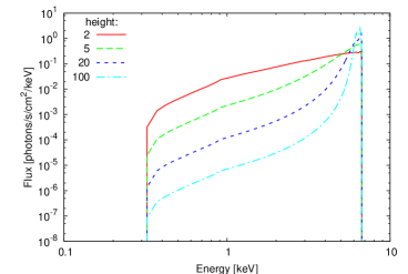
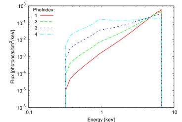
Figure 6: An example of a line profile originating from a disc in equatorial plane of a Kerr black hole ($a=0.9987\,GM/c^{2}$, i.e. $r_{\rm h}=1.05\,GM/c^{2}$) due to the illumination from a primary source on the axis. The kyf1ll model was used. Left: Dependence of the line profile on the height (in $GM/c^{2}$) of a primary source with photon index $\Gamma=2$. Right: Dependence of the line profile on the photon index of the primary emission with a source at height $3\,GM/c^{2}$ above the black hole.

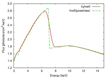
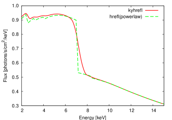
Figure 7: Comparison of the general relativistic kyh1refl model with non-relativistic hrefl(powerlaw). The relativistic blurring of the iron edge is clearly visible. The power-law index of the primary source is PhoIndex=2 (left) and PhoIndex=2.6 (right).

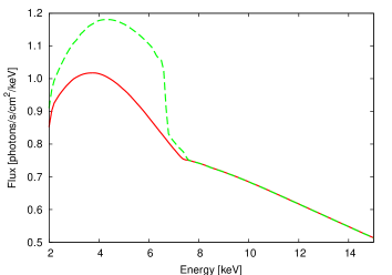
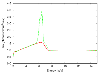
Figure 8: General relativistic lamp-post Compton reflection model kyl1cr with (dashed) and without (solid) iron lines K$\alpha$ and K$\beta$. The emission from the disc is induced by illumination from a primary source placed $2\,GM/c^{2}$ (left) and $100\,GM/c^{2}$ (right) above the black hole.

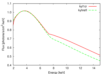
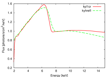
Figure 9: Comparison of the two new general relativistic Compton reflection models kyl1cr and kyh1refl. The lamp-post kyl1cr model is characterized by the height $h$ above the disc where a primary source of emission is placed, the reflection kyh1refl model is characterized by the radial power-law index $\alpha$. Left: $h=2\,GM/c^{2}$, $\alpha=3.4\,$. Right: $h=100\,GM/c^{2}$, $\alpha=1.5\,$.

In our new models we have concentrated ourselves mainly on two components that contribute to the X-ray spectra of active galactic nuclei and X-ray binaries with black-hole candidates – spectral line emission and its relativistic broadening, and the Compton reflection from an illuminated disc. Two basic types of illumination have been considered – the disc illuminated either from every direction by a nearby diffuse corona above the disc, or from a particular direction by a small source placed on the axis above the black hole (see Figure 5). The illumination in the former case decreases with radius as a power law. Hence, this model is characterized by the radial power-law index $\alpha$. On the other hand, the illumination anisotropy in the latter (lamp-post) model depends mainly on the position of a primary source of emission characterized by height $h$ where it is located. In both cases it is assumed that the primary emission has a continuum power-law shape which can be characterized by a photon index $\Gamma$ (PhoIndex).

The emission from the disc depends on quite a number of parameters. It is influenced by the mass $M$ and the rotation $a$ of the central black hole, by the area from which the emission from disc comes (defined by inner radius $r_{\rm in}$, outer radius $r_{\rm out}$ and azimuthal segment with boundaries at $\varphi$ and $\varphi+\Delta\varphi$), by the inclination $\theta_{\rm o}$ of the observer, by the radial power-law index $\alpha$, by the photon index $\Gamma$ and by the position $h$ of a primary source. Limb darkening/brightening law (dependence on the local emission angle) is another important factor that determines the final spectrum we observe.

Here, we will show several examples of emission for the lamp-post fluorescent line model and for the reflection models. For other examples and comparisons, see the accompanying paper (Dovčiak, Karas & Yaqoob [9]). In all figures in this section, we assumed the inclination angle $\theta_{\rm o}=30^{\circ}$, the rotational parameter $a=0.9987\,GM/c^{2}$, and an emitting ring extending from $r_{\rm in}=r_{\rm ms}$ to $r_{\rm out}=400\,GM/c^{2}$.

In Figure 6 we demonstrate that the broad iron emission lines due to illumination from the source placed on the axis depend heavily on the height where the “lamp” is located (left), as well as on the photon index of the primary emission (right). It can be seen that the intrinsic width of the line ($2\,{\rm eV}$ in this example) is much less than its subsequent relativistic broadening, and the local profile (assumed to be Gaussian) is thus smeared in the final spectrum. These graphs correspond to the iron K$\alpha$ line with the rest energy of $6.4$ keV.

Relativistic effects are demonstrated also in Figure 7 where the non-relativistic reflection model hrefl(powerlaw) is compared with our relativistic kyh1refl. Blurring of the iron edge is clearly visible. Here, we set the radial power-law index $\alpha=1$ in kyh1refl. Other parameters defining these models were set to their default values.

Examples of the Compton reflection emission component of the spectra with and without the fluorescent K$\alpha$ and K$\beta$ lines are shown in Figure 8. It can be seen that originally narrow lines can contribute substantially to the continuum component.

We compare the two new relativistic reflection models kyl1cr and kyh1refl in Figure 9. Note that the kyl1cr model is valid only above approximately $2\,{\rm keV}$ and the kyh1refl model only below approximately $15\,{\rm keV}$.

10 Conclusions

In this paper we described the main features of the newly developed set of routines. We have concentrated ourselves on various technical issues connected with fitting X-ray spectra using our model. In particular, we described several variants of the code which are suited for modelling relativistic spectral components originating in a Keplerian disc near a rotating black hole. Both axially symmetric and non-axisymmetric models were discussed. For further details and for exemplary analysis of XMM-Newton satellite data we refer to Dovčiak et al. [9].

Our package offers a number of applications which could not be examined in the limited space of the present paper. In particular, timing analysis can be performed with the code, but we defer detailed description of this capability to subsequent papers. Also, we have only briefly touched the possibility of polarimetric analysis, which offers great possibilities for future X-ray spectroscopy but goes beyond routine capabilities of devices installed onboard present day satellites. Additional emissivity laws can be easily adopted. This can be achieved either by using the convolution component or by adding a new user-defined model. The latter method is more flexible and faster, and hence recommended. In both approaches, the ray-tracing routine is linked and used for relativistic blurring.

As general motivation for developing this project further, we remind the reader that various disc-like structures are almost ubiquitous in objects where the fluid orbits around and inflows onto a compact body. The central mass, $M_{\bullet}$, can vary by many orders of magnitude in different objects, and its value provides the basic classification for black-hole sources. Physical characteristics of accretion discs also scale roughly with $M_{\bullet}$. Indeed, accretion discs around supermassive black holes in active galactic nuclei and quasars share some properties with circumstellar discs in close binary systems, e.g. cataclysmic variable stars and microquasars. However, there are important distinctions between the two kinds of objects which prohibit any simple scaling (for example, galactic nuclear discs tend to be colder and less dense compared to circumstellar discs). In both cases there is strong evidence suggesting that some spectral components (namely, the iron K$\alpha$ line emission) originate, at least in part, within $\sim 10$ gravitational radii of a central black-hole.

The central compact body governs gravitational field in which the medium of an accretion flow evolves. Since we consider a general relativistic description of the gravitational field, the rotation of the central body should not be ignored. An angular momentum is actually one of the model parameters which could in principle be measured by means of spectral analysis of observed radiation.

The authors gratefully acknowledge kind invitation of the meeting organizers and financial support via the Czech Science Foundation grants 205/03/0902 (VK), 202/02/0735 (MD), and from the NASA grants NCC5-447 and NAG5-10769 (TY). Support from the Charles University is also acknowledged (GAUK 299/2004). AM acknowledges financial support from CNES and kind hospitality at the Astronomical Institute of the Czech Academy of Sciences.

Appendix A Appendix

A.1 Summary of equations

Before writing equations for the transfer functions let us summarize basic formulae defining the Kerr space-time, light geodesics and disc’s motion. We remind the reader that units $GM_{\bullet}=c=1$ are used ($M_{\bullet}$ is the mass of the central black hole).

The Kerr metric in Boyer-Lindquist coordinates is

$$g_{\mu\nu}=\left(\begin{array}[]{cccc}-(1-\frac{2r}{\rho^{2}})&0&0&-\frac{2ar\sin^{2}{\!\theta}}{\rho^{2}}\\[5.69054pt] 0&\frac{\rho^{2}}{\Delta}&0&0\\[5.69054pt] 0&0&\rho^{2}&0\\[5.69054pt] -\frac{2ar\sin^{2}{\!\theta}}{\rho^{2}}&0&0&\frac{{\cal A}\sin^{2}{\!\theta}}{\rho^{2}}\end{array}\right)\,,$$

where $\rho^{2}\equiv r^{2}+a^{2}\cos^{2}\!\theta$, $\Delta\equiv r^{2}-2r+a^{2}$ and ${\cal A}\equiv(r^{2}+a^{2})^{2}-\Delta a^{2}\sin^{2}\!\theta$. We assume $0\leq a\leq 1$ everywhere in this paper.

The four-momentum of the photons emitted from the disc is (see e.g. [3] and [23])

$$p_{\rm e}^{t} = [a(l-a)+(r^{2}+a^{2})(r^{2}+a^{2}-al)/\Delta]/r^{2}\,,$$ (A53)

$$p_{\rm e}^{r} = {\rm R}_{\rm sgn}\{(r^{2}+a^{2}-al)^{2}-\Delta[(l-a)^{2}+q^{2}]\}^{1/2}/r^{2}\,,$$ (A54)

$$p_{\rm e}^{\theta} = -q/r^{2}\,,$$ (A55)

$$p_{\rm e}^{\varphi} = [l-a+a(r^{2}+a^{2}-al)/\Delta]/r^{2}\,.$$ (A56)

Here $l=\alpha\sin{\theta_{\rm o}}$ and $q^{2}=\beta^{2}+\cos^{2}{\!(\alpha^{2}-a^{2})}$ are constants of motion with $\alpha$ and $\beta$ being impact parameters measured perpendicular and parallel, respectively, to the spin axis of the black hole projected onto the observer’s sky. Here we define $\alpha$ to be positive when photon travels in the direction of the four-vector $\frac{\partial}{\partial\varphi}$ at infinity, and $\beta$ to be positive if it travels in the direction of $-\frac{\partial}{\partial\theta}$ at infinity. Furthermore, we have denoted sign of the radial component of the momentum by ${\rm R}_{\rm sgn}$. We have chosen an affine parameter along light geodesics in such a way that the conserved energy is normalized to $-p_{{\rm e}\,t}=-p_{{\rm o}\,t}=1$.

The Keplerian velocity of the co-rotating disc above the marginally stable orbit is

$$U^{t} = \frac{r^{2}+a\sqrt{r}}{r\sqrt{r^{2}-3r+2a\sqrt{r}}}\,,$$ (A57)

$$U^{r} = 0\,,$$ (A58)

$$U^{\theta} = 0\,,$$ (A59)

$$U^{\varphi} = \frac{1}{\sqrt{r(r^{2}-3r+2a\sqrt{r})}}\,.$$ (A60)

We assume that the matter in the disc below the marginally stable orbit conserves its specific energy and its specific angular momentum, i.e. $U_{t}(r<r_{\rm ms})=U_{t}(r_{\rm ms})$ and $U_{\varphi}(r<r_{\rm ms})=U_{\varphi}(r_{\rm ms})$. We get the radial component $U^{r}(r<r_{\rm ms})$ from the normalization of the four-velocity, $U^{\mu}\,U_{\mu}=-1$, and from the fact that the disc rotates in the equatorial plane even below the marginally stable orbit, i.e. $U^{\theta}(r<r_{\rm ms})=0$.

In our calculations we use the following local orthonormal tetrad connected with the matter in the disc

$$e_{(t)\,\mu} = U_{\mu}\,,$$ (A61)

$$e_{(r)\,\mu} = \left(\frac{\sqrt{g_{rr}}\,U^{r}U_{t}}{\sqrt{1+U^{r}U_{r}}},\,\sqrt{g_{rr}(1+U^{r}U_{r})},\,0,\,\frac{\sqrt{g_{rr}}\,U^{r}U_{\varphi}}{\sqrt{1+U^{r}U_{r}}}\right)\,,$$ (A62)

$$e_{(\theta)\,\mu} = (0,\,0,\,\sqrt{g_{\theta\theta}},\,0)\,,$$ (A63)

$$e_{(\varphi)\,\mu} = \left(-\frac{\sqrt{\Delta}\,U^{\varphi}}{\sqrt{1+U^{r}U_{r}}},\,0,\,0,\,\frac{\sqrt{\Delta}\,U^{t}}{\sqrt{1+U^{r}U_{r}}}\right)\,.$$ (A64)

The gravitational and Doppler shift ($g$-factor) is defined as the ratio of the energy of a photon received by an observer at infinity to the local energy of the same photon when emitted from an accretion disc

$$g=\frac{\nu_{\rm o}}{\nu_{\rm e}}=\frac{{p_{{\rm o}\,t}}}{{p_{{\rm e}\,\mu}}\,U^{\mu}}=-\frac{1}{{p_{{\rm e}\,\mu}}\,U^{\mu}}\,.$$ (A65)

Here $\nu_{\rm o}$ and $\nu_{\rm e}$ denote frequency of the observed and emitted photons, respectively.

We define lensing as the ratio of the area at infinity perpendicular to the light rays through which photons come to the proper area on the disc perpendicular to the light rays and corresponding to the same flux tube

$$\frac{{\rm d}S_{\rm f}}{{\rm d}S_{\perp}}=\frac{1}{\sqrt{\|Y_{\rm e1}\|^{2}\|Y_{\rm e2}\|^{2}-<Y_{\rm e1},Y_{\rm e2}>^{2}}}\,.$$ (A66)

The four-vectors $Y_{\rm e1}$ and $Y_{\rm e2}$ are transported along the geodesic according to the equation of the geodesic deviation from infinity where they are unit, space-like and perpendicular to each other and to the four-momentum of light. In (A66) we have denoted the magnitude of a four-vector by $\|\ \|$ and the scalar product of two four-vectors by $<\ ,\ >$.

The cosine of the local emission angle is

$$\mu_{\rm e}=\cos{\,\delta_{\rm e}}=-\displaystyle\frac{{p_{{\rm e}\,\alpha}\,n^{\alpha}}}{{p_{{\rm e}\,\mu}\,U^{\mu}}}\,,$$ (A67)

where $n^{\alpha}=-e_{(\theta)}^{\alpha}$ is the normal to the disc with respect to the observer co-moving with the matter in the disc.

The relative time delay $\Delta t$ is the Boyer-Lindquist time which elapses between the emission of a photon from the disc and its reception by an observer (plus a certain constant so that the delay is finite close to the black hole). We have integrated the equation of the geodesics in Kerr ingoing coordinates and thus we have calculated the delay in the Kerr ingoing time coordinate $\Delta t_{\rm K}$. The Boyer-Lindquist time coordinate can be obtained from the Kerr ingoing one by the following equation

$${\rm d}t={\rm d}t_{\rm K}-\left[1+\frac{2r}{(r-r_{+})(r-r_{-})}\right]{\rm d}r\,,$$ (A68)

with $r_{\pm}=1\pm\sqrt{1-a^{2}}$. Then we define the delay as

$$\Delta t = \Delta t_{\rm K}-\left[r+\frac{2}{r_{+}-r_{-}}\,\ln{\frac{r-r_{+}}{r-r_{-}}}+\ln{[(r-r_{+})(r-r_{-})]}\right]\quad{\rm for}\quad a<1\,,$$ (A69)

$$\Delta t = \Delta t_{\rm K}-\left[r-\frac{2}{r-1}+2\ln{(r-1)}\right]\quad{\rm for}\quad a=1\,.$$ (A70)

There is a minus in front of the brackets because the direction of integration is from infinity (represented by $r_{\rm o}=10^{11}$ in our computations) to the disc.

The change of the polarization angle is (see [6], [7])

$$\tan{\Psi}=\frac{Y}{X}\,,$$ (A71)

where

$$X = -(\alpha-a\sin{\theta_{\rm o}})\kappa_{1}-\beta\kappa_{2}\,,$$ (A72)

$$Y = \phantom{-}(\alpha-a\sin{\theta_{\rm o}})\kappa_{2}-\beta\kappa_{1}\,,$$ (A73)

with $\kappa_{1}$ and $\kappa_{2}$ being components of the complex constant of motion $\kappa_{\rm pw}$ (see [29])

$$\kappa_{1} = ar\,p_{\rm e}^{\theta}f^{t}-r\,[a\,p_{\rm e}^{t}-(r^{2}+a^{2})\,p_{\rm e}^{\varphi}]f^{\theta}-r(r^{2}+a^{2})\,p_{\rm e}^{\theta}f^{\varphi}\,,$$ (A75)

$$\kappa_{2} = -r\,p_{\rm e}^{r}f^{t}+r\,[p_{\rm e}^{t}-a\,p_{\rm e}^{\varphi}]f^{r}+ar\,p_{\rm e}^{r}f^{\varphi}\,.$$ (A76)

Here the polarization vector $f^{\mu}$ is a four-vector corresponding to the three-vector $f_{1}$ from Figure 3 which is chosen in such a way that it is a unit vector parallel with $n^{\prime}_{1}$ (i.e. $\Psi_{1}=0$)

$$f^{\mu}=\frac{n^{\mu}-\mu_{\rm e}\left(g\,p_{\rm e}^{\mu}-U^{\mu}\right)}{\sqrt{1-\mu_{\rm e}^{2}}}\,.$$ (A77)

We define the azimuthal emission angle as the angle between the projection of the three-momentum of the emitted photon into the disc (in the local rest frame co-moving with the disc) and the radial tetrad vector:

$$\Phi_{\rm e}=-{\rm R}_{\rm sgn}^{\rm e}\arccos\left(\frac{g\,{p_{{\rm e}\,\alpha}}\,e_{(\varphi)}^{\alpha}}{\sqrt{1-\mu_{\rm e}^{2}}}\right)+\frac{\pi}{2}\,,$$ (A78)

where ${\rm R}_{\rm sgn}^{\rm e}$ is positive if the emitted photon travels outwards ($p_{\rm e}^{(r)}>0$) and negative if it travels inwards ($p_{\rm e}^{(r)}<0$) in the local rest frame of the disc.

We conclude this section by the relationship between the Boyer-Lindquist coordinate $\varphi$ and the Kerr ingoing coordinate $\varphi_{\rm K}$, which we use when we interpolate between the pre-calculated tables

$$\varphi = \varphi_{\rm K}+\frac{a}{r_{+}-r_{-}}\ln{\frac{r-r_{+}}{r-r_{-}}}\quad{\rm for}\quad a<1\,,$$ (A79)

$$\varphi = \varphi_{\rm K}-\frac{1}{r-1}\quad{\rm for}\quad a=1\,.$$ (A80)

A.2 Local emission in lamp-post models

The local emission from a disc is proportional to the incident illumination from a power-law primary source placed on the axis at height $h$ above the black hole. To calculate the incident illumination we need to integrate the geodesics from the source to the disc.

The four-momentum of the incident photons which were emitted by a primary source and which are striking the disc at radius $r$ is (see e.g. [3] and [23])

$$p_{\rm i}^{t} = 1+2/r+4/\Delta\,,$$ (A81)

$$p_{\rm i}^{r} = {\rm R}^{\prime}_{\rm sgn}[(r^{2}+a^{2})^{2}-\Delta(a^{2}+q_{\rm L}^{2})]^{1/2}/r^{2}\,,$$ (A82)

$$p_{\rm i}^{\theta} = q_{\rm L}/r^{2}\,,$$ (A83)

$$p_{\rm i}^{\varphi} = 2a/(r\Delta)\,,$$ (A84)

where $q_{\rm L}^{2}=\sin^{2}{\!\theta_{\rm L}}\,(h^{2}+a^{2})^{2}/\Delta_{\rm L}-a^{2}$ is Carter’s constant of motion with $\Delta_{\rm L}=h^{2}-2h+a^{2}$, and with the angle of emission $\theta_{\rm L}$ being the local angle under which the photon is emitted from a primary source (it is measured in the rest frame of the source). We define this angle by $\tan{\theta_{\rm L}}=-{p_{\rm L}^{(\theta)}/p_{\rm L}^{(r)}}$, where $p_{\rm L}^{(r)}=p_{\rm L}^{\mu}\,e_{{\rm L}\,\mu}^{(r)}$ and $p_{\rm L}^{(\theta)}=p_{\rm L}^{\mu}\,e_{{\rm L}\,\mu}^{(\theta)}$ with $p_{\rm L}^{\mu}$ and $e_{{\rm L}\,\mu}^{(a)}$ being the four-momentum of emitted photons and the local tetrad connected with a primary source, respectively. The angle is $0^{\circ}$ when the photon is emitted downwards and $180^{\circ}$ if the photon is emitted upwards.

We denoted the sign of the radial component of the momentum by ${\rm R}^{\prime}_{\rm sgn}$. We have chosen such an affine parameter for the light geodesic that the conserved energy of the light is $-p_{{\rm i}\,t}=-p_{{\rm L}\,t}=1$. The conserved angular momentum of incident photons is zero ($l_{\rm L}=0$).

The gravitational and Doppler shift of the photons striking the disc which were emitted by a primary source is

$$g_{\rm L}=\frac{\nu_{\rm i}}{\nu_{\rm L}}=\frac{p_{{\rm i}\,\mu}U^{\mu}}{p_{{\rm L}\,\alpha}U_{\rm L}^{\alpha}}=-\frac{p_{{\rm i}\,\mu}U^{\mu}}{U_{\rm L}^{t}}\,.$$ (A85)

Here $\nu_{\rm i}$ and $\nu_{\rm L}$ denote the frequency of the incident and emitted photons, respectively and $U_{\rm L}^{\alpha}$ is a four-velocity of the primary source with the only non-zero component $U_{\rm L}^{t}=\sqrt{\frac{h^{2}+a^{2}}{\Delta_{\rm L}}}$.

The cosine of the local incident angle is

$$\mu_{\rm i}=|\cos{\delta_{\rm i}}\,|=\displaystyle\frac{{p_{{\rm i}\,\alpha}\,n^{\alpha}}}{{p_{{\rm i}\,\mu}\,U^{\mu}}}\,,$$ (A86)

where $n^{\alpha}=-e_{(\theta)}^{\alpha}$ is normal to the disc with respect to the observer co-moving with the matter in the disc.

We further define the azimuthal incident angle as the angle between the projection of the three-momentum of the incident photon into the disc (in the local rest frame co-moving with the disc) and the radial tetrad vector,

$$\Phi_{\rm i}=-{\rm R}_{\rm sgn}^{\rm i}\arccos\left(\frac{-1}{\sqrt{1-\mu_{\rm i}^{2}}}\frac{\,{p_{{\rm i}\,\alpha}}\,e_{(\varphi)}^{\alpha}}{p_{{\rm i}\,\mu}U^{\mu}}\right)+\frac{\pi}{2}\,,$$ (A87)

where ${\rm R}_{\rm sgn}^{\rm i}$ is positive if the incident photon travels outwards ($p_{\rm i}^{(r)}>0$) and negative if it travels inwards ($p_{\rm i}^{(r)}<0$) in the local rest frame of the disc.

In lamp-post models the emission of the disc will be proportional to the incident radiation $N_{\rm i}^{S}(E_{\rm l})$ which comes from a primary source

$$N_{\rm i}^{S}(E_{\rm l})=N_{\rm L}^{\Omega}(E_{\rm L})\frac{{\rm d}\Omega_{\rm L}}{{\rm d}S_{{\rm l}}}\,.$$ (A88)

Here $N_{\rm L}^{\Omega}(E_{\rm L})=N_{0{\rm L}}\,E_{\rm L}^{-\Gamma}$ is an isotropic and stationary power-law emission from a primary source which is emitted into a solid angle ${\rm d}\Omega_{\rm L}$ and which illuminates local area ${\rm d}S_{\rm l}$ on the disc. The energy of the photon striking the disc (measured in the local frame co-moving with the disc) will be redshifted

$$E_{\rm l}=g_{\rm L}\,E_{\rm L}\,.$$ (A89)

The ratio ${\rm d}\Omega_{\rm L}/{\rm d}S_{{\rm l}}$ is

$$\frac{{\rm d}\Omega_{\rm L}}{{\rm d}S_{{\rm l}}}=\frac{{\rm d}\Omega_{\rm L}}{{\rm d}S}\frac{{\rm d}S}{{\rm d}S_{\rm l}}=\frac{\sin{\theta_{\rm L}{\rm d}\theta_{\rm L}\,{\rm d}\varphi}}{{\rm d}r\,{\rm d}\varphi}\frac{{\rm d}S}{{\rm d}S_{\rm l}}\,,$$ (A90)

where (see eqs. (5) and (7))

$${\rm d}S={\rm d}r\,{\rm d}\varphi=|{\rm d}^{2}{\!S_{t}}^{\theta}|=-g^{\theta\theta}\,\frac{p_{{\rm i}t}}{p_{\rm i}^{\theta}}\,{\rm d}S_{\perp}=\,\frac{g^{\theta\theta}}{p_{\rm i}^{\theta}}\,{\rm d}S_{\perp}\,.$$ (A91)

Here we used the same space-time slice as in the discussion above eq. (4) and thus the element ${\rm d}^{2}\!S_{\alpha\beta}$ is defined as before, see eq. (5). Note that here the area ${\rm d}S_{\perp}$ is defined by the incident flux tube as opposed to ${\rm d}S_{\perp}$ in eq. (8) where it was defined by the emitted flux tube. The coordinate area ${\rm d}S$ corresponds to the proper area ${\rm d}S_{\perp}$ which is perpendicular to the incident light ray (in the local rest frame co-moving with the disc). The corresponding proper area (measured in the same local frame) lying in the equatorial plane will be

$${\rm d}S_{{\rm l}} = |{\rm d}^{2}{\!S_{(t)}}^{\!\!(\theta)}|=|e_{(t)}^{\mu}\,e^{{(\theta)}\,\nu}\,{\rm d}^{2}\!S_{\mu\nu}|=|g_{\theta\theta}^{-1/2}\,U^{\mu}\,{\rm d}^{2}\!S_{\mu\theta}|=$$ (A92)

$$= -g_{\theta\theta}^{-1/2}\,\frac{p_{{\rm i}\mu}\,U^{\mu}}{p_{\rm i}^{\theta}}\,{\rm d}S_{\perp}=g_{\theta\theta}^{-1/2}\frac{U_{\rm L}^{t}}{p_{\rm i}^{\theta}}\,g_{\rm L}\,{\rm d}S_{\perp}\,.$$

Here we have used eq. (4) for the tetrad components of the element ${\rm d}^{2}\!S_{\alpha\beta}$, eqs. (6) and (A85).

It follows from eqs. (A88)–(A92) that the incident radiation will be again a power law with the same photon index $\Gamma$ as in primary emission

$$N_{\rm i}^{S}(E_{{\rm l}})=N_{0{\rm i}}\,E_{{\rm l}}^{-\Gamma}\,,$$ (A93)

with the normalization factor

$$N_{0{\rm i}}=N_{0{\rm L}}\,g_{\rm L}^{\Gamma-1}\,\sqrt{1-\frac{2h}{h^{2}+a^{2}}}\,\frac{\sin{\theta_{\rm L}}\,{\rm d}\theta_{\rm L}}{r\,{\rm d}r}\,.$$ (A94)

The emission of the disc due to illumination will be proportional to this factor.

A.3 Description of FITS files

A.3.1 Transfer functions in KBHtablesNN.fits

The transfer functions are stored in the file KBHtablesNN.fits as binary extensions and parametrized by the value of the observer inclination angle $\theta_{\rm o}$ and the horizon of the black hole $r_{\rm h}$. We found parametrization by $r_{\rm h}$ more convenient than using the rotational parameter $a$, although the latter choice may be more common. Each extension provides values of a particular transfer function for different radii, which are given in terms of $r-r_{\rm h}$, and for the Kerr ingoing axial coordinates $\varphi_{\rm K}$. Values of the horizon $r_{\rm h}$, inclination $\theta_{\rm o}$, radius $r-r_{\rm h}$ and angle $\varphi_{\rm K}$, at which the functions are evaluated, are defined as vectors at the beginning of the FITS file.

The definition of the file KBHtablesNN.fits:

1. All of the extensions defined below are binary.

2. The first extension contains six integers defining which of the functions is present in the tables. The integers correspond to the delay, $g$-factor, cosine of the local emission angle, lensing, change of the polarization angle and azimuthal emission angle, respectively. Value $0$ means that the function is not present in the tables, value $1$ means it is.

3. The second extension contains a vector of the horizon values in $GM/c^{2}$ ($1.00\leq r_{\rm h}\leq 2.00$).

4. The third extension contains a vector of the values of the observer’s inclination angle $\theta_{\rm o}$ in degrees ($0^{\circ}\leq\theta_{\rm o}\leq 90^{\circ}$, $0^{\circ}$ – axis, $90^{\circ}$ – equatorial plane).

5. The fourth extension contains a vector of the values of the radius relative to the horizon $r-r_{\rm h}$ in $GM/c^{2}$.

6. The fifth extension contains a vector of the values of the azimuthal angle $\varphi_{\rm K}$ in radians ($0\leq\varphi_{\rm K}\leq 2\pi$). Note that $\varphi_{\rm K}$ is a Kerr ingoing axial coordinate, not the Boyer-Lindquist one!

7. All the previous vectors have to have values sorted in an increasing order.

8. In the following extensions the transfer functions are defined, each extension is for a particular value of $r_{\rm h}$ and $\theta_{\rm o}$. The values of $r_{\rm h}$ and $\theta_{\rm o}$ are changing with each extension in the following order:
   $r_{\rm h}[1]\times\theta_{\rm o}[1]$, $r_{\rm h}[1]\times\theta_{\rm o}[2]$, $r_{\rm h}[1]\times\theta_{\rm o}[3]$, … … $r_{\rm h}[2]\times\theta_{\rm o}[1]$, $r_{\rm h}[2]\times\theta_{\rm o}[2]$, $r_{\rm h}[2]\times\theta_{\rm o}[3]$, … …

9. Each of these extensions has the same number of columns (up to six). In each column, a particular transfer function is stored – the delay, $g$-factor, cosine of the local emission angle, lensing, change of the polarization angle and azimuthal emission angle, respectively. The order of the functions is important but some of the functions may be missing as defined in the first extension (see 1. above). The functions are:

   delay

   – the Boyer-Lindquist time in $GM/c^{3}$ that elapses between the emission of a photon from the disc and absorption of the photon by the observer’s eye at infinity plus a constant,

   $g$-factor

   – the ratio of the energy of a photon received by the observer at infinity to the local energy of the same photon when emitted from an accretion disc,

   cosine of the emission angle

   – the cosine of the local emission angle between the emitted light ray and local disc normal,

   lensing

   – the ratio of the area at infinity perpendicular to the light rays through which photons come to the proper area on the disc perpendicular to the light rays and corresponding to the same flux tube,

   change of the polarization angle in radians

   – if the light emitted from the disc is linearly polarized then the direction of polarization will be changed by this angle at infinity – counter-clockwise if positive, clockwise if negative (we are looking towards the coming emitted beam); on the disc we measure the angle of polarization with respect to the “up” direction perpendicular to the disc with respect to the local rest frame; at infinity we also measure the angle of polarization with respect to the “up” direction perpendicular to the disc – the change of the polarization angle is the difference between these two angles,

   azimuthal emission angle in radians

   – the angle between the projection of the three-momentum of an emitted photon into the disc (in the local rest frame co-moving with the disc) and the radial tetrad vector.

   For mathematical formulae defining the functions see eqs. (A65), (A66)–(A67), (A69)–(A71) and (A78) in Appendix A.1.

10. Each row corresponds to a particular value of $r-r_{\rm h}$ (see 4. above).

11. Each element corresponding to a particular column and row is a vector. Each element of this vector corresponds to a particular value of $\varphi_{\rm K}$ (see 5. above).

We have pre-calculated three sets of tables – KBHtables00.fits, KBHtables50.fits and KBHtables99.fits. All of these tables were computed for an accretion disc near a Kerr black hole with no disc corona present. Therefore, ray-tracing in the vacuum Kerr space-time could be used for calculating the transfer functions. When computing the transfer functions, it was supposed that the matter in the disc rotates on stable circular (free) orbits above the marginally stable orbit. The matter below this orbit is freely falling and has the same energy and angular momentum as the matter which is on the marginally stable orbit.

The observer is placed in the direction $\varphi=\pi/2$. The black hole rotates counter-clockwise. All six functions are present in these tables.

Tables are calculated for these values of the black-hole horizon:
– KBHtables00.fits: 1.00, 1.05, 1.10, 1.15, …, 1.90, 1.95, 2.00 (21 elements),
– KBHtables50.fits: 1.00, 1.10, 1.20, …, 1.90, 2.00 (11 elements),
– KBHtables99.fits: 1.05 (1 element),
and for these values of the observer’s inclination:
– KBHtables00.fits: 0.1, 1, 5, 10, 15, 20, …, 80, 85, 89 (20 elements),
– KBHtables50.fits: 0.1, 1, 10, 20, …, 80, 89 (11 elements),
– KBHtables99.fits: 0.1, 1, 5, 10, 15, 20, …, 80, 85, 89 (20 elements).

The radii and azimuths at which the functions are evaluated are same for all three tables:
– radii $r-r_{\rm h}$ are exponentially increasing from 0 to 999 (150 elements),
– values of the azimuthal angle $\varphi_{\rm K}$ are equidistantly spread from 0 to $2\pi$ radians with a much denser cover “behind” the black hole, i.e. near $\varphi_{\rm K}=1.5\pi$ (because some of the functions are changing heavily in this area for higher inclination angles, $\theta_{\rm o}>70^{\circ}$) (200 elements).

A.3.2 Tables in KBHlineNN.fits

Pre-calculated functions ${\rm d}F(g)\equiv{\rm d}g\,F(g)$ defined in eq. (16) are stored in FITS files KBHlineNN.fits. These functions are used by all axisymmetric models. They are stored as binary extensions and they are parametrized by the value of the observer inclination angle $\theta_{\rm o}$ and the horizon of the black hole $r_{\rm h}$. Each extension provides values for different radii, which are given in terms of $r-r_{\rm h}$, and for different $g$-factors. Values of the $g$-factor, radius $r-r_{\rm h}$, horizon $r_{\rm h}$, and inclination $\theta_{\rm o}$, at which the functions are evaluated, are defined as vectors at the beginning of the FITS file.

The definition of the file KBHlineNN.fits:

1. All of the extensions defined below are binary.

2. The first extension contains one row with three columns that define bins in the $g$-factor:

   • integer in the first column defines the width of the bins (0 – constant, 1 – exponentially growing),

   • real number in the second column defines the lower boundary of the first bin (minimum of the $g$-factor),

   • real number in the third column defines the upper boundary of the last bin (maximum of the $g$-factor).

3. The second extension a contains vector of the values of the radius relative to the horizon $r-r_{\rm h}$ in $GM/c^{2}$.

4. The third extension contains a vector of the horizon values in $GM/c^{2}$ ($1.00\leq r_{\rm h}\leq 2.00$).

5. The fourth extension contains a vector of the values of the observer’s inclination angle $\theta_{\rm o}$ in degrees ($0^{\circ}\leq\theta_{\rm o}\leq 90^{\circ}$, $0^{\circ}$ – axis, $90^{\circ}$ – equatorial plane).

6. All the previous vectors have to have values sorted in an increasing order.

7. In the following extensions the functions ${\rm d}F(g)$ are defined, each extension is for a particular value of $r_{\rm h}$ and $\theta_{\rm o}$. The values of $r_{\rm h}$ and $\theta_{\rm o}$ are changing with each extension in the same order as in tables in the KBHtablesNN.fits file (see the previous section, point 7.). Each extension has one column.

8. Each row corresponds to a particular value of $r-r_{\rm h}$ (see 2. above).

9. Each element corresponding to a particular column and row is a vector. Each element of this vector corresponds to a value of the function for a particular bin in the $g$-factor. This bin can be calculated from number of elements of the vector and data from the first extension (see 1. above).

We have pre-calculated several sets of tables for different limb darkening/brightening laws and with different resolutions. All of them were calculated from tables in the KBHtables00.fits (see the previous section for details) and therefore these tables are calculated for the same values of the black-hole horizon and observer’s inclination. All of these tables have equidistant bins in the $g$-factor which fall in the interval $\langle 0.001,1.7\rangle$. Several sets of tables are available:
– KBHline00.fits for isotropic emission, see eq. (29),
– KBHline01.fits for Laor’s limb darkening, see eq. (30),
– KBHline02.fits for Haardt’s limb brightening, see eq. (31).
All of these tables have 300 bins in the $g$-factor and 500 values of the radius $r-r_{\rm h}$ which are exponentially increasing from 0 to 999. We have produced also tables with a lower resolution – KBHline50.fits, KBHline51.fits and KBHline52.fits with 200 bins in the $g$-factor and 300 values of the radius.

A.3.3 Lamp-post tables in lamp.fits

This file contains pre-calculated values of the functions needed for the lamp-post model. It is supposed that a primary source of emission is placed on the axis at a height $h$ above the Kerr black hole. The matter in the disc rotates on stable circular (free) orbits above the marginally stable orbit and it is freely falling below this orbit where it has the same energy and angular momentum as the matter which is on the marginally stable orbit. It is assumed that the corona between the source and the disc is optically thin, therefore ray-tracing in the vacuum Kerr space-time could be used for computing the functions.

There are five functions stored in the lamp.fits file as binary extensions. They are parametrized by the value of the horizon of the black hole $r_{\rm h}$, and height $h$, which are defined as vectors at the beginning of the FITS file. Currently only tables for $r_{\rm h}=1.05$ (i.e. $a\doteq 0.9987492$) and $h=2,\,3,\,4,\,5,\,6,\,8,\,10,\,12,\,15,\,20,\,30,\,50,\,75$ and $100$ are available. The functions included are:

• – the angle under which a photon is emitted from a primary source placed at a height $h$ on the axis above the black hole measured by a local stationary observer ($0^{\circ}$ – a photon is emitted downwards, $180^{\circ}$ – a photon is emitted upwards),

• – the radius in $GM/c^{2}$ at which a photon strikes the disc,

• – the ratio of the energy of a photon hitting the disc to the energy of the same photon when emitted from a primary source,

• – an absolute value of the cosine of the local incident angle between the incident light ray and local disc normal,

• – the angle between the projection of the three-momentum of the incident photon into the disc (in the local rest frame co-moving with the disc) and the radial tetrad vector.

For mathematical formulae defining the functions see eqs. (A85)–(A87) in Appendix A.2.

The definition of the file lamp.fits:

1. All of the extensions defined below are binary.

2. The first extension contains a vector of the horizon values in $GM/c^{2}$, though currently only FITS files with tables for one value of the black-hole horizon are accepted ($1.00\leq r_{\rm h}\leq 2.00$).

3. The second extension contains a vector of the values of heights $h$ of a primary source in $GM/c^{2}$.

4. In the following extensions the functions are defined. Each extension is for a particular value of $r_{\rm h}$ and $h$. The values of $r_{\rm h}$ and $h$ are changing with each extension in the following order:
   $r_{\rm h}[1]\times h[1]$, $r_{\rm h}[1]\times h[2]$, $r_{\rm h}[1]\times h[3]$, … … $r_{\rm h}[2]\times h[1]$, $r_{\rm h}[2]\times h[2]$, $r_{\rm h}[2]\times h[3]$, … …

5. Each of these extensions has five columns. In each column, a particular function is stored – the angle of emission, radius, $g$-factor, cosine of the local incident angle and azimuthal incident angle, respectively. Extensions may have a different number of rows.

A.3.4 Coefficient of reflection in fluorescent_line.fits

Values of the coefficient of reflection $f(\mu_{\rm i},\mu_{\rm e})$ for a fluorescent line are stored for different incident and reflection angles in this file. For details on the model of scattering used for computations see [21]. It is assumed that the incident radiation is a power law with the photon index $\Gamma=1.7$. The coefficient does not change its angular dependences for other photon indices, only its normalization changes (see Figure 14 in [12]). The FITS file consists of three binary extensions:

• the first extension contains absolute values of the cosine of incident angles,

• the second extension contains values of the cosine of reflection angles,

• the third extension contains one column with vector elements, here values of the coefficient of reflection are stored for different incident angles (rows) and for different reflection angles (elements of a vector).

A.3.5 Tables in refspectra.fits

The function $f(E_{\rm l};\mu_{\rm i},\mu_{\rm e})$ which gives dependence of a locally emitted spectrum on the angle of incidence and angle of emission is stored in this FITS file. The emission is induced by a power-law incident radiation. Values of this function were computed by the Monte Carlo simulations of Compton scattering, for details see [21]. The reflected radiation depends on the photon index $\Gamma$ of the incident radiation. There are several binary extensions in this FITS file:

• the first extension contains energy values in keV where the function $f(E_{\rm l};\mu_{\rm i},\mu_{\rm e})$ is computed, currently the interval from 2 to 300 keV is covered,

• the second extension contains the absolute values of the cosine of the incident angles,

• the third extension contains the values of the cosine of the emission angles,

• the fourth extension contains the values of the photon indices $\Gamma$ of the incident power law, currently tables for $\Gamma=1.5,\,1.6,\,\dots,\,2.9$ and $3.0$ are computed,

• in the following extensions the function $f(E_{\rm l};\mu{\rm i},\mu_{\rm e})$ is defined, each extension is for a particular value of $\Gamma$; here values of the function are stored as a vector for different incident angles (rows) and for different angles of emission (columns), each element of this vector corresponds to a value of the function for a certain value of energy.

A.4 Description of the integration routines

Here we describe the technical details about the integration routines, which act as a common driver performing the ray-tracing for various models of the local emission. The description of non-axisymmetric and axisymmetric versions are both provided. An appropriate choice depends on the form of intrinsic emissivity. Obviously, non-axisymmetric tasks are computationally more demanding.

A.4.1 Non-axisymmetric integration routine ide

This subroutine integrates the local emission and local Stokes parameters for (partially) polarized emission of the accretion disc near a rotating (Kerr) black hole (characterized by the angular momentum $a$) for an observer with an inclination angle $\theta_{\rm o}$. The subroutine has to be called with ten parameters:

ide(ear,ne,nt,far,qar,uar,var,ide_param,emissivity,ne_loc)

ear

– real array of energy bins (same as ear for local models in xspec),

ne

– integer, number of energy bins (same as ne for local models in xspec),

nt

– integer, number of grid points in time (${\tt nt}=1$ means stationary model),

far(ne,nt)

– real array of photon flux per bin (same as photar for local models in xspec but with the time resolution),

qar(ne,nt)

– real array of the Stokes parameter Q divided by the energy,

uar(ne,nt)

– real array of the Stokes parameter U divided by the energy,

var(ne,nt)

– real array of the Stokes parameter V divided by the energy,

ide_param

– twenty more parameters needed for the integration (explained below),

emissivity

– name of the external emissivity subroutine, where the local emission of the disc is defined (explained in detail below),

ne_loc

– number of points (in energies) where local photon flux (per keV) in the emissivity subroutine is defined.

The description of the ide_param parameters follows:

ide_param(1)

– a/M – the black-hole angular momentum ($0\leq{\tt a/M}\leq 1$),

ide_param(2)

– theta_o – the observer inclination in degrees ($0^{\circ}$ – pole, $90^{\circ}$ – equatorial plane),

ide_param(3)

– rin-rh – the inner edge of the non-zero disc emissivity relative to the black-hole horizon (in $GM/c^{2}$),

ide_param(4)

– ms – determines whether we also integrate emission below the marginally stable orbit; if its value is set to zero and the inner radius of the disc is below the marginally stable orbit then the emission below this orbit is taken into account, if set to unity it is not,

ide_param(5)

– rout-rh – the outer edge of the non-zero disc emissivity relative to the black-hole horizon (in $GM/c^{2}$),

ide_param(6)

– phi – the position angle of the axial sector of the disc with non-zero emissivity in degrees,

ide_param(7)

– dphi – the inner angle of the axial sector of the disc with non-zero emissivity in degrees (${\tt dphi}\leq 360^{\circ}$),

ide_param(8)

– nrad – the radial resolution of the grid,

ide_param(9)

– division – the switch for the spacing of the radial grid ($0$ – equidistant, $1$ – exponential),

ide_param(10)

– nphi – the axial resolution of the grid,

ide_param(11)

– smooth – the switch for performing simple smoothing ($0$ – no, $1$ – yes),

ide_param(12)

– normal – the switch for normalizing the final spectrum,
if $=$ 0 – total flux is unity (usually used for the line),
if $>$ 0 – flux is unity at the energy = normal keV (usually used for the continuum),
if $<$ 0 – final spectrum is not normalized,

ide_param(13)

– zshift – the overall redshift of the object,

ide_param(14)

– ntable – tables to be used, it defines a double digit number NN in the name of the FITS file KBHtablesNN.fits containing the tables ($0\leq{\tt ntable}\leq 99$),

ide_param(15)

– edivision – the switch for spacing the grid in local energies (0 – equidistant, 1 – exponential),

ide_param(16)

– periodic – if set to unity then local emissivity is periodic if set to zero it is not (need not be set if ${\tt nt}=1$),

ide_param(17)

– dt – the time step (need not be set if ${\tt nt}=1$),

ide_param(18)

– polar – whether the change of the polarization angle and/or azimuthal emission angle will be read from FITS tables (0 – no, 1 – yes),

ide_param(19)

– r0-rh and

ide_param(20)

– phi0 – in dynamical computations the initial time will be set to the time when photons emitted from the point [r0, phi0] on the disc (in the Boyer-Lindquist coordinates) reach the observer.

The ide subroutine needs an external emissivity subroutine in which the local emission and local Stokes parameters are defined. This subroutine has twelve parameters:
     emissivity( ear_loc,ne_loc,nt,far_loc,qar_loc,uar_loc,var_loc,r,phi,cosine, phiphoton,first_emis)

ear_loc(0:ne_loc)

– real array of the local energies where local photon flux far_loc is defined, with special meaning of ear_loc(0) – if its value is larger than zero then the local emissivity consists of two energy regions where the flux is non-zero; the flux between these regions is zero and ear_loc(0) defines the number of points in local energies with the zero local flux,

ne_loc

– integer, the number of points (in energies) where the local photon flux (per keV) is defined,

nt

– integer, the number of grid points in time (${\tt nt}=1$ means stationary model),

far_loc(0:ne_loc,nt)

– real array of the local photon flux (per keV) – if the local emissivity consists of two separate non-zero regions (i.e. ${\tt ear\_loc(0)}>0$) then far_loc(0,it) is the index of the last point of the first non-zero local energy region,

qar_loc(ne_loc,nt)

– real array of the local Stokes parameter Q divided by the local energy,

uar_loc(ne_loc,nt)

– real array of the local Stokes parameter U divided by the local energy,

var_loc(ne_loc,nt)

– real array of the local Stokes parameter V divided by the local energy,

r

– the radius in $GM/c^{2}$ where the local photon flux far_loc at the local energies ear_loc is demanded

phi

– the azimuth (the Boyer-Lindquist coordinate $\varphi$) where the local photon flux far_loc at the local energies ear_loc is demanded,

cosine

– the cosine of the local angle between the emitted ray and local disc normal,

phiphoton

– the angle between the emitted ray projected onto the plane of the disc (in the local frame of the moving disc) and the radial component of the local tetrad (in radians),

first_emis

– boolean, TRUE if we enter the emissivity subroutine from the ide subroutine for the first time, FALSE if this subroutine was already evaluated during the present run. This distinction is convenient to initialize some variables when calling the emissivity subroutine for the first time (e.g. calculation of the falling spot trajectory can be performed in this place).

A.4.2 Axisymmetric integration routine idre

This subroutine integrates the local axisymmetric emission of an accretion disc near a rotating (Kerr) black hole (characterized by the angular momentum $a$) for an observer with an inclination angle $\theta_{\rm o}$. The subroutine has to be called with eight parameters:

idre(ear,ne,photar,idre_param,cmodel,ne_loc,ear_loc,far_loc)

ear

– real array of energy bins (same as ear for local models in xspec),

ne

– integer, the number of energy bins (same as ne for local models in xspec),

photar

– real array of the photon flux per bin (same as photar for local models in xspec),

idre_param

– ten more parameters needed for the integration (explained below),

cmodel

– 32-byte string with a base name of a FITS file with tables for axisymmetric emission (e.g. “KBHline” for KBHlineNN.fits),

ne_loc

– the number of points (in energies) where the local photon flux (per keV) is defined in the emissivity subroutine,

ear_loc

– array of the local energies where the local photon flux far_loc is defined

far_loc

– array of the local photon flux (per keV).

The description of the idre_param parameters follows:

idre_param(1)

– a/M – the black-hole angular momentum ($0\leq{\tt a/M}\leq 1$),

idre_param(2)

– theta_o – the observer inclination in degrees ($0^{\circ}$ – pole, $90^{\circ}$ – equatorial plane),

idre_param(3)

– rin-rh – the inner edge of the non-zero disc emissivity relative to the black-hole horizon (in $GM/c^{2}$),

idre_param(4)

– ms – determines whether we also integrate emission below the marginally stable orbit; if its value is set to zero and the inner radius of the disc is below the marginally stable orbit then the emission below this orbit is taken into account, if set to unity it is not,

idre_param(5)

– rout-rh – the outer edge of the non-zero disc emissivity relative to the black-hole horizon (in $GM/c^{2}$),

idre_param(6)

– smooth – the switch for performing simple smoothing ($0$ – no, $1$ – yes),

idre_param(7)

– normal – the switch for normalizing the final spectrum,
if $=$ 0 – total flux is unity (usually used for the line),
if $>$ 0 – flux is unity at the energy = normal keV (usually used for the continuum),
if $<$ 0 – final spectrum is not normalized,

idre_param(8)

– zshift – the overall redshift of the object,

idre_param(9)

– ntable – tables to be used, it defines a double digit number NN in the name of the FITS file (e.g. in KBHlineNN.fits) containing the tables ($0\leq{\tt ntable}\leq 99$),

idre_param(10)

– alpha – the radial power-law index.

The idre subroutine does not need for its operation any external emissivity subroutine.

References

- [1] Arnaud K. A., 1996. XSPEC: The first ten years. In Astronomical Data Analysis Software and Systems V, eds. Jacoby G. & Barnes J., ASP Conf. Series, vol. 101, p. 17
- [2] Beckwith K., & Done C., 2004. Iron line profiles in strong gravity. MNRAS, in press (astro-ph/0402199)
- [3] Carter B., 1968. Global structure of the Kerr family of gravitational fields. Phys. Rev., 174, 1559
- [4] Chandrasekhar S. 1960. Radiative Transfer. Dover publications, New York
- [5] Chandrasekhar S., 1992. The Mathematical Theory of Black Holes. New York, Oxford University Press
- [6] Connors P. A., & Stark R. F., 1977. Observable gravitational effects on polarized radiation coming from near a black hole. Nature, 269, 128
- [7] Connors P. A., Piran T., & Stark R. F., 1980. Polarization features of X-ray radiation emitted near black holes. ApJ, 235, 224
- [8] Dovčiak M., 2004. PhD Thesis (Charles University, Prague), in preparation
- [9] Dovčiak M., Karas V., & Yaqoob T., 2004. An extended scheme for fitting X-ray data with accretion disc spectra in the strong gravity regime. ApJS, 153, 205
- [10] Fabian A. C., Iwasawa K., Reynolds C. S., & Young A. J., 2000. Broad iron lines in active galactic nuclei. PASP, 112, 1145
- [11] Fanton C., Calvani M., de Felice F., & Čadež A., 1997. Detecting accretion discs in active galactic nuclei. PASJ, 49, 159
- [12] George I. M., & Fabian A. C., 1991. X-ray reflection from cold matter in active galactic nuclei and X-ray binaries. MNRAS, 249, 352
- [13] Ghisellini G., Haardt F., & Matt G., 1994. The contribution of the obscuring torus to the X-ray spectrum of Seyfert galaxies – a test for the unification model. MNRAS, 267, 743
- [14] Gierliński M., Maciolek-Niedźwiecki A., & Ebisawa K., 2001. Application of a relativistic accretion disc model to X-ray spectra of LMC X-1 and GRO J1655-40. MNRAS, 325, 1253
- [15] Haardt F. 1993. Anisotropic Comptonization in thermal plasmas – Spectral distribution in plane-parallel geometry. ApJ, 413, 680
- [16] Kato S., Fukue J., & Mineshige S., 1998. Black-Hole Accretion Discs. Kyoto, Kyoto Univ. Press
- [17] Krolik J. H., 1999. Active Galactic Nuclei. Princeton University Press, Princeton
- [18] Laor A., Netzer H., & Piran, T., 1990. Massive thin accretion discs. II – Polarization. MNRAS, 242, 560
- [19] Laor A. 1991. Line profiles from a disc around a rotating black hole. ApJ, 376, 90
- [20] Martocchia A., Karas V., & Matt G., 2000. Effects of Kerr space-time on spectral features from X-ray illuminated accretion discs. MNRAS, 312, 817
- [21] Matt G., Perola G. C., & Piro L., 1991. The iron line and high energy bump as X-ray signatures of cold matter in Seyfert 1 galaxies. A&A, 247, 25
- [22] Matt G., Perola G. C., Piro L., & Stella L., 1992. Iron K-alpha line from X-ray illuminated relativistic discs. A&A, 257, 63; ibid. 1992, 263, 453
- [23] Misner C. W., Thorne K. S., & Wheeler J. A., 1973. Gravitation. San Fransisco, W.H.Freedman & Co.
- [24] Novikov I. D., & Thorne K. S., 1973. In Black Holes, eds. DeWitt C., DeWitt B. S. New York, Gordon & Breach, p. 343
- [25] Phillips K. C., & Mészáros P., 1986. Polarization and beaming of accretion disc radiation. ApJ, 310, 284
- [26] Rauch K. P., & Blandford R. D., 1994. Optical caustics in a Kerr space-time and the origin of rapid X-ray variability in active galactic nuclei. ApJ, 421, 46
- [27] Reynolds C. S., & Nowak M. A., 2003. Fluorescent iron lines as a probe of astrophysical black hole systems. Phys. Rep., 377, 389
- [28] Schnittman J. D., & Bertschinger E., 2004. The harmonic structure of high-frequency quasi-periodic oscillations in accreting black holes. ApJ, 606, 1098
- [29] Walker M., & Penrose R., 1970. On quadratic first integrals of the geodesic equations for type {22} spacetimes. Commun. Math. Phys., 18, 265