Lithium-6 and Gamma Rays:
Complementary Constraints on Cosmic-Ray History

Abstract

The rare isotope ${}^{6}{\rm Li}$ is made only by cosmic rays, dominantly in $\alpha\alpha\rightarrow\mbox{${}^{6}{\rm Li}$}$ fusion reactions with ISM helium. Consequently, this nuclide provides a unique diagnostic of the history of cosmic rays in our Galaxy. The same hadronic cosmic-ray interactions also produce high-energy $\gamma$ rays (mostly via $pp\rightarrow\pi^{0}\rightarrow\gamma\gamma$). Thus, hadronic $\gamma$-rays and ${}^{6}{\rm Li}$ are intimately linked. Specifically, ${}^{6}{\rm Li}$ directly encodes the local cosmic-ray fluence over cosmic time, while extragalactic hadronic $\gamma$ rays encode an average cosmic-ray fluence over lines of sight out to the horizon. We examine this link and show how ${}^{6}{\rm Li}$ and $\gamma$-rays can be used together to place important model-independent limits on the cosmic-ray history of our Galaxy and the universe. We first constrain $\gamma$-ray production from ordinary Galactic cosmic rays, using the local ${}^{6}{\rm Li}$ abundance. We find that the solar ${}^{6}{\rm Li}$ abundance demands an accompanying extragalactic pionic $\gamma$-ray intensity which exceeds that of the entire observed EGRB by a factor of $2-6$. Possible explanations for this discrepancy are discussed. We then constrain Li production using recent determinations of extragalactic $\gamma$-ray background (EGRB). We note that cosmic rays created during cosmic structure formation would lead to pre-Galactic Li production, which would act as a “contaminant” to the primordial ${}^{7}{\rm Li}$ content of metal-poor halo stars; the EGRB can place an upper limit on this contamination if we attribute the entire EGRB pionic contribution to structure forming cosmic rays. Unfortunately, the uncertainties in the determination of the EGRB are so large that the present $\gamma$-ray data cannot guarantee that the pre-Galactic Li is small compared to primordial ${}^{7}{\rm Li}$; thus, an improved determination of the EGRB will shed important new light on this issue. Our limits and their more model-dependent extensions will improve significantly with additional observations of ${}^{6}{\rm Li}$ in halo stars, and with improved measurements of the EGRB spectrum by GLAST.

1 Introduction

The origin and history of cosmic rays has been a subject of intensifying interest. For more than a decade, a large body of work has focused on the light elements Li, Be, and B (LiBeB) as signatures of cosmic-ray interactions with the diffuse gas (for a recent review see Cassé, Vangioni-Flam, & Audouze, 2001). LiBeB abundances in Galactic halo stars have been used to probe the history of cosmic rays in the (proto-)Galaxy. More recently, a great deal of attention has been focused on high-energy $\gamma$-rays also produced in interactions during cosmic-ray propagation. Here, we draw attention to the tight connection between these observables, particularly between $\gamma$-rays and ${}^{6}{\rm Li}$.

The abundances of LiBeB nuclei encode the history of cosmic ray exposure in local matter. In the past 15 years or so, measurements of LiBeB in the Sun and in Galactic disk have been joined by LiBeB observations in halo stars; these offer particularly valuable information about cosmic-ray origins and interactions in Galactic and proto-Galactic matter. In particular, different scenarios for cosmic ray origin lead to different LiBeB trends, which have been modeled and compared with observations (see, e.g., Vangioni-Flam & Cassé, 2001; Fields & Olive, 1999a; Ramaty, Scully, Lingenfelter, & Kozlovsky, 2000, and references therein). For the purposes of this paper, the details of these models are less important than the following basic distinction: all LiBeB species are produced as cosmic rays interact with interstellar gas and fragment–“spall”–heavy nuclei, e.g., $p+{\rm O}\rightarrow\mbox{${}^{9}{\rm Be}$}$. However, the fusion processes $\alpha+\alpha\rightarrow\mbox{${}^{6,7}{\rm Li}$}$ yield lithium isotopes exclusively, and indeed dominate the cosmic-ray production of Li (Steigman & Walker, 1992; Montmerle, 1977c). This makes cosmic-ray lithium production particularly “clean” since its evolution depends uniquely on its exposure to cosmic rays, and unlike Be and B, does not depend on the ambient heavy element abundances.

Cosmic-ray interactions provide the only known source for the nucleosynthesis of ${}^{6}{\rm Li}$, ${}^{9}{\rm Be}$, and ${}^{10}{\rm B}$, making these species ideal observables of cosmic ray activity. The story is more complex for ${}^{11}{\rm B}$, which can also be produced in core-collapse supernovae by the “neutrino process” (e.g., Woosley, Hartmann, Hoffman, & Haxton, 1990; Yoshida, Terasawa, Kajino, & Sumiyoshi, 2004). Finally, ${}^{7}{\rm Li}$ has the most diverse lineage. In the early Galaxy, and hence in halo stars, ${}^{7}{\rm Li}$ is dominated by the contribution from primordial nucleosynthesis (e.g., Cyburt, Fields, & Olive, 2003, and references therein), with a small contribution from cosmic-ray fusion as well as the neutrino process (Ryan et al., 2000). At late times, and hence in disk stars including the Sun, ${}^{7}{\rm Li}$ has important and probably dominant contributions from longer-lived, low-mass stars (though the specific site remains controversial: Romano, Matteucci, Ventura, & D’Antona, 2001; Travaglio et al., 2001). In this paper we will build on the work of Suzuki & Inoue (2002) to point out the possible importance of another, pre-Galactic, source of cosmic-ray ${}^{7}{\rm Li}$ and ${}^{6}{\rm Li}$, which could confound attempts to identify the pre-Galactic Li abundance with the primordial component. We cannot rule out (or in!) this possible source, but we will constrain it using observations of $\gamma$-rays.

Cosmic-ray interactions with interstellar gas produce not only LiBeB, but also inevitably produce $\gamma$-rays. Cosmic rays in the Galactic disk today lead to pronounced emission seen in the Galactic plane (Hunter et al., 1997). Cosmic ray populations in (and between!) external galaxies would contribute to a diffuse extragalactic $\gamma$-ray background (hereafter the EGRB). The existence of an EGRB was already claimed by some of the first $\gamma$-ray observations (Fichtel, Kniffen, & Hartman, 1973). The most recent high-energy (i.e., roughly in the 30 MeV – 30 GeV range) $\gamma$-ray observations are those of the EGRET experiment on the Compton Gamma-Ray Observatory, and the EGRET team also found evidence for a EGRB (Sreekumar et al., 1998). The intensity, energy spectrum, and even the existence of an EGRB are not trivial to measure, as this information only arises as the residual after subtracting the dominant Galactic foreground from the observed $\gamma$-ray sky. The procedure for foreground subtraction is thus crucial, and different procedures starting with the same EGRET data have arrived at an EGRB with a lower intensity and different spectrum (Strong, Moskalenko, & Reimer, 2004), or have even failed to find evidence for an EGRB at all (Keshet, Waxman, & Loeb, 2003). Despite these uncertainties, we will see that the EGRB (or limits to it) and Li abundances are mutually very constraining.

Whether or not an EGRB has yet been detected, at some level it certainly should exist. EGRET detections of individual active galactic nuclei (blazars) as well as the Milky Way and the LMC together guarantee that unresolved blazars (e.g., Stecker & Salamon, 1996; Mukherjee & Chiang, 1999), and to a lesser extent normal galaxies (Pavlidou & Fields, 2002), will generate a signal at or near the levels claimed for the EGRB. Many other EGRB sources have been proposed, but one of the promising has been a subject of intense interest recently: namely, $\gamma$-rays originating from a cosmological component of cosmic rays. This as-yet putative cosmic-ray population would originate in shocks (Miniati et al., 2000; Keshet et al., 2003; Ryu, Kang, Hallman, & Jones, 2003) associated with baryonic infall and merger events during the growth of large-scale cosmic structures. Diffusive shock acceleration (e.g., Blasi, 2004; Kang, Jones, & Gieseler, 2002; Jones & Ellison, 1991) would then generate a population of relativistic ions and electrons. Gamma-ray emission would then follow from inverse Compton scattering of electrons off of the ambient photon backgrounds and from $\pi^{0}$ production due to hadronic collisions (Loeb & Waxman, 2000). The most recent semi-analytical and numerical calculations (Gabici & Blasi, 2003; Miniati, 2002) suggest that this “structure forming” component to the EGRB is likely below the blazar contribution, but the observational and theoretical uncertainties here remain large; upcoming $\gamma$-ray observations by GLAST (Gehrels & Michelson, 1999) will shed welcome new light on this problem.

The link between the nucleosynthesis and $\gamma$-ray signatures of cosmic-ray history has been pointed out by others in multiple contexts. We note in particular the prescient work of Montmerle (1977a, b, c), who in a series of papers considered the implications of a hypothetical population of “cosmological cosmic rays” in addition to the usual Galactic cosmic rays. Montmerle’s analysis is impressive in its foresight and its breadth. Montmerle (1977a) develops the formalism for a homogeneous population of cosmological cosmic rays (assumed to be created instantaneously at some redshift), and describes their propagation in an expanding universe, as well as their light element and $\gamma$-ray production. He identifies the tight connection between ${}^{6}{\rm Li}$ and extragalactic $\gamma$-rays, and exploits this connection to use the available EGRB data to constrain Li production for a variety of different assumptions. A particularly pertinent case involves an EGRB near the levels discussed today (“normalization 2” in Montmerle’s parlance), coupled with a cosmic baryon density close to modern values (e.g., Spergel et al., 2003; Cyburt, Fields, & Olive, 2003). Under these conditions, Montmerle (1977b) finds that cosmological cosmic ray activity sufficient to explain the EGRB leads to a present ${}^{6}{\rm Li}$ abundance that is about an order of magnitude smaller than the solar abundance. This result foreshadows an important conclusion we will find: if the solar ${}^{6}{\rm Li}$ abundance is produced by Galactic cosmic rays, then the associated pionic $\gamma$-ray production exceeds the entire EGRB by at least a factor of 2.

More recently, studies of structure formation cosmic rays have focused primarily on their $\gamma$-ray signatures. However, recently Suzuki & Inoue (2002) also proposed using ${}^{6}{\rm Li}$ as a diagnostic of shock activity in the Local Group. These authors note that the resulting ${}^{6}{\rm Li}$ abundances in halo stars could be used to probe the shocks and resulting cosmic rays in proto-Galactic matter. We also will draw on this idea, with an emphasis on the fact that pre-Galactic Li production would be (by itself) observationally indistinguishable from the primordial ${}^{7}{\rm Li}$ production from big bang nucleosynthesis. Thus we attempt to use EGRB data to constrain this possibility, but find that current data is unable to rule out a significant contribution to halo star Li abundances from structure formation cosmic rays.

Our work thus follows these pioneering efforts, further emphasizing and formally exploring the intimate connection between cosmic-ray nucleosynthesis and high-energy $\gamma$-ray astrophysics. In §2, we formally show and discuss the generality and tightness of the ${}^{6}{\rm Li}$-$\gamma$ connection, and in §3 the relevant observations are reviewed. In §4 we use the theory of LiBeB production by Galactic cosmic rays to deduce the minimal contribution the EGRB. In §5 we exploit the link to use the observed EGRB to limit the SFCR contribution to pre-Galactic lithium. Discussion and conclusions appear in §6.

2 The Gamma-Ray – Lithium Connection: Formalism

Before doing a detailed calculation let us first establish a simple, back of the envelope, connection between gamma-rays and lithium. We know that low energy ($\sim 10-100$ MeV/nucleon) hadronic cosmic rays produce lithium through $\alpha\alpha\rightarrow\mbox{${}^{6,7}{\rm Li}$}+\cdots$. But higher-energy ($>280$ MeV/nucleon) cosmic rays also produce $\gamma$-rays via neutral pion decay: $pp\rightarrow\pi^{0}\rightarrow\gamma\gamma$. Because they share a common origin in hadronic cosmic ray interactions, we can directly relate cosmic ray lithium production to “pionic” gamma-rays. The cosmic-ray production rate of ${}^{6}{\rm Li}$ per unit volume is $q({\mbox{${}^{6}{\rm Li}$}})=\sigma_{\alpha\alpha\rightarrow{}^{6}{\rm Li}}\Phi_{\alpha}n_{\alpha}$, where $\Phi_{\alpha}$ is the net cosmic ray He flux, $n_{\alpha}$ is the interstellar He abundance, and $\sigma_{\alpha\alpha\rightarrow{}^{6}{\rm Li}}$ is the cross section for ${}^{6}{\rm Li}$ production, appropriately averaged over the cosmic-ray energy spectrum (detailed definitions and normalization conventions appear in Appendix A). Thus, the ${}^{6}{\rm Li}$ mole fraction $Y_{6}=n_{6}/n_{\rm b}$ is just $Y({\mbox{${}^{6}{\rm Li}$}})\sim\int\frac{dt}{n_{b}}q_{\mbox{${}^{6}{\rm Li}$}}\sim y_{\alpha,\rm cr}Y_{\alpha,\rm ism}\sigma_{\alpha\alpha\rightarrow{}^{6}{\rm Li}}\Phi_{p}t_{0}$. where $y_{\alpha,\rm cr}=\Phi_{\alpha}/\Phi_{p}\approx{\rm(He/H)_{ism}}$.

On the other hand, the cosmic-ray production rate of pionic $\gamma$-rays is just the pion production rate times a factor of 2, that is, $q_{\gamma}=2\sigma_{pp\rightarrow\pi^{0}}\Phi_{p,\rm cr}n_{p,\rm ism}$. Integrated over a line of sight towards the cosmic particle horizon, this gives a EGRB intensity $I_{\gamma}\sim c\int dtq_{\gamma}/4\pi\sim 2\sigma_{pp\rightarrow\pi^{0}}c\Phi_{p}t_{0}$. Thus we see that both the ${}^{6}{\rm Li}$ abundance and the $\gamma$-ray intensity have a common factor of the (time-integrated) cosmic-ray flux, and so we can eliminate this factor and express each observable in terms of the other:

$$Y_{\mbox{${}^{6}{\rm Li}$}}\sim y_{\alpha,{\rm cr}}Y_{\alpha,{\rm gas}}\frac{2\pi}{n_{b}c}\frac{\sigma_{\mbox{${}^{6}{\rm Li}$}}^{\alpha\alpha}}{\sigma_{\pi^{0}}^{pp}}I_{\gamma}$$ (1)

From eq. (1) we see that the connection between cosmic-ray lithium production and pionic gamma-ray flux is straight forward.

This rough argument shows the intimacy of the connection between ${}^{6}{\rm Li}$ and pionic $\gamma$-rays. However, this simplistic treatment does not account for the expansion of the universe, nor for time-variations in the cosmic-cosmic ray flux, nor for the inhomogeneous distribution of sources within the universe. We now include these effects in a more rigorous treatment.

For Li production at location $\vec{x}$, the production rate per unit (physical) volume is

$$q_{\rm Li}(\vec{x})=\sigma_{\alpha\alpha}\Phi_{\alpha}^{\rm cr}(\vec{x})n_{\rm\alpha,gas}(\vec{x})=y_{\alpha,\rm cr}Y_{\alpha}^{\rm ism}\sigma_{\alpha\alpha}\Phi_{p}^{\rm cr}(\vec{x})n_{\rm b,gas}(\vec{x})\equiv\mu(\vec{x})\Gamma_{\rm Li}(\vec{x})n_{\rm b}(\vec{x})$$ (2)

Here, $y_{\alpha,\rm cr}=(\alpha/p)_{\rm cr}$ is the cosmic-ray He/H ratio, and is assumed to be constant in space and time. The target density of (interstellar or intergalactic) helium is $n_{\rm\alpha,gas}$, which we write in terms of its ratio $Y_{\alpha}^{\rm ism}=n_{\rm He}/n_{\rm b}$ to the baryon density. We take $Y_{\alpha}^{\rm ism}\approx 0.06$ to be constant in space and time, but we do not assume this for the baryon density $n_{\rm b}(\vec{x})$. The baryonic gas fraction

$$\mu=n_{\rm b,gas}/n_{\rm b}$$ (3)

accounts for the fact that not all baryons need to be in a diffuse form. Finally, we will find it convenient to write $q_{\rm Li}(\vec{x})$ in terms of the local baryon density and the local Li production rate $\Gamma_{\rm Li}(\vec{x})$ per baryon.

With these expressions, we have

$$\frac{d}{dt}Y_{\rm Li}(\vec{x})=\mu(\vec{x})\Gamma_{\rm Li}(\vec{x})$$ (4)

which we can solve to get

$$Y_{\rm Li}(\vec{x},t) = \int_{0}^{t}dt^{\prime}\ \mu(\vec{x},t^{\prime})\ \Gamma_{\rm Li}(\vec{x},t^{\prime})$$ (5)

$$= y_{\alpha,\rm cr}Y_{\alpha}^{\rm ism}\sigma_{\alpha\alpha}\int_{0}^{t}dt^{\prime}\ \mu(\vec{x},t^{\prime})\ \Phi_{p}^{\rm cr}(\vec{x},t^{\prime})$$ (6)

$$= y_{\alpha,\rm cr}Y_{\alpha}^{\rm ism}\sigma_{\alpha\alpha}F_{p}({\vec{x}},t)$$ (7)

where $F_{p}(\vec{x},t)=\int_{0}^{t}dt^{\prime}\ \mu(\vec{x},t^{\prime})\ \Phi_{p}^{\rm cr}(\vec{x},t^{\prime})$ is the local proton fluence (time-integrated flux), weighted by the gas fraction. Thus we see that Li (and particularly ${}^{6}{\rm Li}$) serves as a “cosmic-ray dosimeter” which measures the net local cosmic ray exposure.

We now turn to $\gamma$ rays from hadronic sources, most of which come from neutral pion production and decay: $pp\rightarrow\pi^{0}\rightarrow\gamma\gamma$. The extragalactic background due to these process is expected to be isotropic (at least to a good approximation). In this case, the total $\gamma$-ray intensity $I_{\gamma}=dN_{\gamma}/dA\,dt\,d\Omega$, integrated over all energies, is given by an integral

$$I_{\gamma}(t)=\frac{c}{4\pi}\int_{0}^{t}dt^{\prime}\ q_{\gamma}^{\rm com}(t^{\prime})$$ (8)

of the sources over the line of sight to the horizon. We are interested in particular in the case of hadronic sources, so that $q_{\rm com}=a^{3}q$ is the total (energy-integrated) comoving rate of hadronic $\gamma$-ray production per unit volume; here $a$ is the usual cosmic scale factor, which we normalize to a present value of $a_{0}=a(t_{0})=1$. A formal derivation of eq. (8) appears in Appendix B, but one can arrive at this result from elementary considerations. Namely, note that the comoving number density of photons produced at any point is just $n_{\gamma,\rm com}=\int_{0}^{t}q_{\gamma}^{\rm com}\,dt^{\prime}$. We neglect photon absorption and scattering processes, and thus particle number conservation along with homogeneity and isotropy together demand that the comoving number density of ambient photons at any point is the same as the comoving number density of photons produced there. Furthermore, the total (energy-integrated) photon intensity is also isotropic and thus by definition is $I_{\gamma}=n_{\gamma,\rm com}c/4\pi$, which is precisely what we find in eq.  (8).

The comoving rate of pionic $\gamma$-ray production per unit volume at point $\vec{s}$ is

$$q_{\gamma}^{\rm com}(\vec{s},t)=\sigma_{\gamma}\Phi_{p}(\vec{s},t)n_{\rm H,gas}^{\rm com}(\vec{s},t)=\mu(\vec{s},t)\sigma_{\gamma}\Phi_{p}(\vec{s},t)n_{\rm H}^{\rm com}(\vec{s},t)$$ (9)

where $n_{\rm H}$ is the (comoving) hydrogen density, and $\Phi_{p}=4\pi\int I_{p}(\epsilon_{\rm rest})d\epsilon_{\rm rest}$ is the total (integrated over rest-frame energy $\epsilon_{\rm rest}$) omnidirectional cosmic ray proton flux. The flux-averaged pionic $\gamma$-ray production cross section is

$$\sigma_{\gamma}\equiv 2\xi_{\alpha}\zeta_{\pi}\sigma_{\pi^{0}}=2\xi_{\alpha}\frac{\int d\epsilon_{\rm rest}\,I_{p}(\epsilon_{\rm rest})\,\zeta_{\pi}\sigma_{\pi^{0}}(\epsilon_{\rm rest})}{\int d\epsilon_{\rm rest}\,I_{p}(\epsilon_{\rm rest})}$$ (10)

where the factor of 2 counts the number of photons per pion decay, $\sigma_{\pi^{0}}$ is the cross section for pion production and $\zeta_{\pi}$ is the pion multiplicity, and the factor $\xi_{\alpha}=1.45$ accounts for $p\alpha$ and $\alpha\alpha$ reactions (Dermer, 1986).

Then we have

$$I_{\gamma}(t)=\frac{n_{\rm b,0}c}{4\pi}Y_{\rm H}\sigma_{\gamma}\int_{0}^{t}dt\ \mu(\vec{s})\ \frac{n_{\rm b}^{\rm com}(\vec{s})}{n_{\rm b,0}}\ \Phi_{p}(\vec{s},t)=\frac{n_{\rm b,0}c}{4\pi}\sigma_{\gamma}Y_{H}^{\rm ism}F_{p}(t)$$ (11)

where

$$F_{p}(t)=\int_{0}^{t}dt\ \mu(\vec{s})\ \frac{n_{\rm b}^{\rm com}(\vec{s})}{n_{\rm b,0}}\ \Phi_{p}(\vec{s})$$ (12)

is a mean value of the cosmic-ray fluence along the line of sight, where the average is weighted by the gas fraction and the ratio $n_{\rm b}^{\rm com}(\vec{s})/n_{\rm b,0}$ of the local baryon density along the photon path. Note that the $\gamma$-ray sources are sensitive to the overlap of the cosmic-ray flux with the diffuse hydrogen gas density, and thus need not be homogeneous. Even so, we still assume the ERGB intensity to be isotropic, which corresponds to the assumption that the line-of-sight integral over the sources averages out any fluctuations.

One further technical note: $I_{\gamma}\equiv I_{\gamma}(>0)=\int_{0}^{\infty}d\epsilon_{\gamma}I_{\gamma}(\epsilon_{\gamma})$ represents the total pionic $\gamma$-ray flux, integrated over photon energies. While this quantity is well-defined theoretically, real observations have some energy cutoff, and thus report $I_{\gamma}(>\epsilon_{0})=\int_{\epsilon_{0}}^{\infty}d\epsilon_{\gamma}I_{\gamma}(\epsilon_{\gamma})$, typically with $\epsilon_{0}=100$ MeV. But the spectrum of pionic $\gamma$-rays will be shifted towards lower energies if they originate from a nonzero redshift. Thus it is clear that $\gamma$-ray intensity $I_{\gamma}$, integrated above some energy $\epsilon_{0}\neq 0$, will be redshift-dependent. A way to eliminate this $z$-dependence is to include all pionic $\gamma$-rays, that is to take $I_{\gamma}\equiv I_{\gamma}(>0\rm\ GeV)$, i.e., to take $\epsilon_{0}=0$. As discussed in more detail in Appendix B, the ${}^{6}{\rm Li}$-$\gamma$ proportionality is only exact for $I_{\gamma}(>0)$, as this quantity removes photon redshifting effects which spoil the proportionality for $\epsilon_{0}\neq 0$. Thus we will have to use information on the pionic spectrum to translate between $I_{\gamma}(>\epsilon_{0})$ and $I_{\gamma}(>0)$; these issues are discussed further in §3.1.

Thus we see that the lithium abundance and the pionic $\gamma$-ray intensity (spectrum integrated from 0 energy) arise from very similar integrals, which we can express via the ratio

$$\frac{I_{\gamma}(t)}{Y_{i}(\vec{x},t)}=\frac{n_{\rm b}c}{4\pi y_{\alpha,\rm cr}y_{\alpha,\rm ism}}\ \frac{\sigma_{\gamma}}{\sigma_{\alpha\alpha}^{i}}\ \frac{F_{p}(t)}{F_{p}(\vec{x},t)}$$ (13)

where $i$ denotes ${}^{6}{\rm Li}$ or ${}^{7}{\rm Li}$. Note that this “$\gamma$-to-lithium” ratio has its only significant space and time dependence via the ratio $F_{p}(t)/F_{p}(\vec{x},t)$ of the line-of-sight baryon-averaged fluence to the local fluence.

The relationship expressed in eq. (13) is the main result of this paper, and we will bring this tool to bear on Li and $\gamma$-ray observations, using each to constrain the other. To do this, it will be convenient to write eq. (13) in the form

$$I_{\gamma}(t)=I_{0,i}\frac{Y_{i}(\vec{x},t)}{Y_{i,\odot}}\frac{F_{p}(t)}{F_{p}(\vec{x},t)}$$ (14)

where the scaling factor

$$I_{0,i}=\frac{n_{\rm b}c}{4\pi y_{\alpha,\rm cr}y_{\alpha,\rm ism}}\ \frac{\sigma_{\gamma}}{\sigma_{\alpha\alpha}^{i}}\ Y_{i,\odot}$$ (15)

is independent of time and space, and only depends, via the ratio of cross sections, on the shape of the cosmic-ray population considered. Table 1 presents the values of $I_{0,i}$ for the different spectra that will be considered in the following sections. Values of the scaling factor were obtained by using photon multiplicity $\xi_{\gamma}=2$, $\zeta_{\alpha}=1.45$, baryon number density $n_{\rm b}=2.52\times 10^{-7}\ \rm cm^{-3}$, CR and ISM helium abundances $y_{\rm\alpha}^{\rm cr}=y_{\rm\alpha}^{\rm ism}=0.1$ and solar abundances $y_{\mbox{${}^{6}{\rm Li}$}_{\odot}}=1.53\times 10^{-10}$ and $y_{\mbox{${}^{7}{\rm Li}$}_{\odot}}=1.89\times 10^{-9}$ (Anders & Grevesse, 1989). For the $\pi^{0}$ and lithium production cross-sections, we used the fits taken from Dermer (1986) and Mercer et al. (2001), and from that obtained the ratios of flux-averaged cross-sections for different spectra, and these are also presented in Table 1.

Table 1: Lithium and $\gamma$-ray Scalings and Production Ratios

Cosmic-Ray	$\rm I_{0,6}$	$\rm I_{0.7}$
Population	$[\rm cm^{-2}s^{-1}sr^{-1}]$		$\sigma_{\mbox{${}^{6}{\rm Li}$}}^{\alpha\alpha}/\sigma_{\pi}^{pp}$	$\sigma_{\mbox{${}^{7}{\rm Li}$}}^{\alpha\alpha}/\sigma_{\pi}^{pp}$	${}^{7}{\rm Li}$/${}^{6}{\rm Li}$
GCR	$9.06\times 10^{-5}$	$8.36\times 10^{-4}$	0.21	0.28	1.3
SFCR	$1.86\times 10^{-5}$	$1.15\times 10^{-4}$	1.02	2.03	2.0

Table 1 shows that the different cosmic-ray spectra lead to very different Li-to-$\gamma$ ratios. For example, the ${}^{6}{\rm Li}$-to-$\gamma$ ratio $\sigma_{\mbox{${}^{6}{\rm Li}$}}^{\alpha\alpha}/\sigma_{\pi}^{pp}$ is almost a factor of 5 higher in the SFCR case than in the GCR case. The reason for this stems from the different threshold behaviors and energy dependences of the Li and $\pi^{0}$ production cross sections. Li production via $\alpha\alpha$ fusion has a threshold around 10 MeV/nucleon, above which the cross section rapidly rises through some resonant peaks. Then beyond $\sim 15$ MeV/nucleon, the cross section for ${}^{6}{\rm Li}$ drops exponentially as $e^{-E/{16\ \rm MeV/nucleon}}$(Mercer et al., 2001), rapidly suppressing the importance of any projectiles with $E\gg 16$ MeV/nucleon. Thus, as has been widely discussed, Li production is a low-energy phenomenon for which the important projectile energy range is roughly $10-70$ MeV/nucleon.

On the other hand, $pp\rightarrow\pi^{0}$ production has a higher threshold of 280 MeV, and the effective cross section $\zeta_{\pi}\sigma_{pp}^{\pi}$ rises with energy up to and beyond 1 GeV. Neutral pion production is thus a significantly higher-energy phenomenon.

These different cross section behaviors are sensitive to the differences in the two cosmic-ray spectra we adopt. On the one hand, we adopt a GCR spectrum that is a power law in total energy: $\phi_{p}(E)\propto(m_{p}+E)^{-2.75}$, a good approximation to the locally observed (i.e., propagated) spectrum. This spectrum is roughly constant for $E<m_{p}$. Thus, there is no reduction in cosmic-ray flux between the Li and $\pi^{0}$ thresholds. Furthermore the flux only begins to drop far above the $\pi^{0}$ threshold at 280 MeV, so that there is significant pion production over a large range of energies, in contrast to the intrinsically narrow energy window for Li production. As a result of the effects, $\sigma_{\mbox{${}^{6}{\rm Li}$}}^{\alpha\alpha}/\sigma_{\pi}^{pp}\ll 1$ for the GCR case.

In contrast, the SFCR flux is taken to be the standard result for diffusive acceleration due to a strong shock: namely, a power law in momentum $\phi(E)\propto p(E)^{-2}$. This goes to $\phi\propto E^{-1}$ at $E\mathrel{\mathchoice{\lower 3.6pt\vbox{\halign{$\mathsurround=0pt\displaystyle\hfil#\hfil$\cr<\crcr\sim\crcr}}}{\lower 3.6pt\vbox{\halign{$\mathsurround=0pt\textstyle\hfil#\hfil$\cr<\crcr\sim\crcr}}}{\lower 3.6pt\vbox{\halign{$\mathsurround=0pt\scriptstyle\hfil#\hfil$\cr<\crcr\sim\crcr}}}{\lower 3.6pt\vbox{\halign{$\mathsurround=0pt\scriptscriptstyle\hfil#\hfil$\cr<\crcr\sim\crcr}}}}m_{p}$, and $\phi\propto E^{-2}$ at higher energies. This spectrum thus drops by a factor of 28 between the Li and $\pi^{0}$ thresholds, and continues to drop above the $\pi^{0}$ threshold, offsetting the rise in the pion cross section. This behavior thus suppresses $\pi^{0}$ production relative to the GCR case, and thus we have a significantly higher $\sigma_{\mbox{${}^{6}{\rm Li}$}}^{\alpha\alpha}/\sigma_{\pi}^{pp}$ ratio. As we will see, these ratios–and the differences between them–will be critical in deriving quantitative constraints.

3 Observational Inputs

We have seen that the EGRB intensity and lithium abundances are closely linked. Here we collect information on both observables.

3.1 The Observed Gamma-Ray Background and Limits to the Pionic Contribution

Ever since $\gamma$-rays were first observed towards the Galactic poles as well as in the plane (Fichtel, Kniffen, & Hartman, 1973), the existence of emission at high Galactic latitudes has been regarded as an indication of an EGRB. However, any information regarding the intensity, energy spectrum, and even the existence of the EGRB is only as reliable as the procedure for subtracting the Galactic foreground. Such procedures are unfortunately non-trivial and model-dependent. The EGRET team (Sreekumar et al., 1998) used an empirical model for tracers of Galactic hydrogen and starlight, and found evidence for an EGRB which dominates polar emission. Other groups have recently presented new analyses of the EGRET data. In a semi-empirical approach using a model of Galactic $\gamma$-ray sources, Strong, Moskalenko, & Reimer (2004) also find evidence for an EGRB, but with a different energy spectrum and a generally lower intensity than the Sreekumar et al. (1998) result. Finally, Keshet, Waxman, & Loeb (2003) find that the Galactic foreground is sufficiently uncertain that its contribution to the polar emission can be significant, possibly saturating the observations. Consequently, the Keshet, Waxman, & Loeb (2003) analysis is unable to confirm the existence of an EGRB in the EGRET data; instead, they can only to place upper limits on the EGRB intensity.

It was recently shown by Prodanović & Fields (2004) that a model-independent limit on the fraction of EGRB flux that is of pionic origin (gamma rays that originate from $\pi^{0}$ decay) can be placed. Their limit comes from noticing that the EGRB shows no strong evidence of the distinctive shape pionic $\gamma$-ray spectral peak at $m_{\pi^{0}}/2$, the “pion bump.” Thus by comparing the shapes of the observed EGRB and theoretical pionic gamma-ray spectrum, they were able to maximize the pionic flux so that it stays below the observed one. This procedure allowed them to place constraints on the maximal fraction of EGRB that can be of pionic origin.

For the pionic $\gamma$-ray source-function, Prodanović & Fields (2004) used a semi-analytic fit from the Pfrommer & Enßlin (2003) paper and the Dermer (1986) model for the production cross section. A key feature of the pionic $\gamma$-ray spectrum is that it approaches a power law at both high and low energies, going to $\epsilon^{\alpha_{\gamma}}$ for $\epsilon\ll m_{\pi}/2$ and to $\epsilon^{-\alpha_{\gamma}}$ for $\epsilon\gg m_{\pi}/2$. In Dermer’s model, the $\gamma$-ray spectral index $\alpha_{\gamma}$ is equal to the cosmic-ray spectral index. Prodanović & Fields (2004) adopted the value $\alpha_{\gamma}=2.2$ for pionic extragalactic $\gamma$-rays, which is consistent with blazars and structure-forming cosmic rays as their origin. In this simple analysis, Prodanović & Fields (2004) used a single-redshift approximation, that is, they assumed that these $\gamma$-rays are all coming from one redshift, and thus their limit on the maximal pionic fraction is a function of $z$.

To obtain the EGRB spectrum from EGRET data, a careful subtraction of Galactic foreground is needed. Prodanović & Fields (2004) considered two different EGRB spectra and obtained the following limit : for the Sreekumar et al. (1998) spectrum they found that the pionic fraction of the EGRB (integrated spectra above 100 MeV) can be as low as about 40% for cosmic rays that originated at present, to about 90 % for $z=10$; for the more shallow spectrum of Strong, Moskalenko, & Reimer (2004) they found that pionic fraction can go from about 30% for $z=0$ up to about 70% for $z=10$. However, the Keshet, Waxman, & Loeb (2003) analysis of the EGRET data implies that the Galactic foreground dominates the $\gamma$-ray sky so that only an upper limit on the EGRB can be placed, namely $I_{\gamma}(>100\rm MeV)\leq 0.5\times 10^{-5}\ \ \rm cm^{-2}\ s^{-1}\ sr^{-1}$. Thus, in this case, we were not able to obtain the pionic fraction.

However, to be able to connect the pionic $\gamma$-ray intensity $I_{\gamma}$ with lithium mole fraction $Y_{i}$ as shown in (13), $I_{\gamma}$ must include all of the pionic $\gamma$-rays, that is, the spectrum has to be integrated from energy $\epsilon_{0}=0$. The upper limit to the pionic $\gamma$-ray intensity above energy $\epsilon_{0}$ for a given redshift can be written as

$$I_{\gamma}(>\epsilon_{0}) = f_{\pi}(>\epsilon_{0},z)I_{\gamma}^{\rm obs}(>\epsilon_{0})$$ (16)

$$= \mathcal{N}_{\rm max}\int_{\epsilon_{0}}\varphi[\epsilon(1+z)]d\epsilon$$ (17)

where $f_{\pi}(>\epsilon_{0},z)$ is the upper limit to the fraction of pionic $\gamma$-rays (Prodanović & Fields, 2004), $I_{\gamma}^{\rm obs}(>\epsilon_{0})$ is the observed intensity above some energy, while $\varphi[\epsilon(1+z)]$ is the semi-analytic fit for pionic $\gamma$-ray spectrum (Pfrommer & Enßlin, 2003) which is maximized with $\mathcal{N}_{\rm max}$ normalization constant. An upper limit to the pionic $\gamma$-ray intensity that covers all energies $I_{\gamma}(>0,z)$, follows immediately from the above equations:

$$I_{\gamma}(>0,z)=f_{\pi}(>\epsilon_{0},z)I_{\gamma}^{\rm obs}(>\epsilon_{0})\frac{\int_{0}\varphi[\epsilon(1+z)]d\epsilon}{\int_{\epsilon_{0}}\varphi[\epsilon(1+z)]d\epsilon}$$ (18)

Now this is something that is semi-observational and can be easily obtained from $\gamma$-ray intensity observed above some energy, and from Prodanović & Fields (2004) and Pfrommer & Enßlin (2003) results.

3.2 The Primordial Lithium Abundance

Given the EGRB intensity, we will infer the amount of associated lithium production. It will be of interest to compare this not only to the solar abundance, but also to the primordial abundance of ${}^{7}{\rm Li}$. Metal-poor halo stars (extreme Population II) serve as a “fossil record” of pre-Galactic lithium. Ryan et al. (2000) find a pre-Galactic abundance

$$\left(\frac{\rm Li}{\rm H}\right)_{\rm pre-Gal,obs}=(1.23^{+0.34}_{-0.16})\times 10^{-10}$$ (19)

based on an analysis of very metal-poor halo stars. On the other hand, one can use the WMAP (Spergel et al., 2003) baryon density and BBN to predict a “theoretical” (or “CMB-based”) primordial ${}^{7}{\rm Li}$ abundance (Cyburt, Fields, & Olive, 2003):

$$\left(\frac{\mbox{${}^{7}{\rm Li}$}}{\rm H}\right)_{\rm BBN,thy}=(3.82^{+0.73}_{-0.60})\times 10^{-10}$$ (20)

These abundances are clearly inconsistent. Possible explanations for this discrepancy include unknown or underestimated systematic errors in theory and/or observations or new physics; these are discussed thoroughly elsewhere (see, e.g., Cyburt, Fields, & Olive, 2003, and refs therein). For our purposes, we will acknowledge this discrepancy by comparing pre-Galactic lithium production by cosmic rays with both the observed and CMB-based Li abundances.

4 ${}^{6}{\rm Li}$ and Gamma-Rays From Galactic Cosmic Rays

We have shown that ${}^{6}{\rm Li}$ abundances and extragalactic $\gamma$-rays are linked because both sample cosmic-ray fluence, and now apply this formalism to $\gamma$-ray and ${}^{6}{\rm Li}$ data. In this section we turn to the hadronic products of Galactic cosmic rays, which are believed to be the dominant source of ${}^{6}{\rm Li}$, but a sub-dominant contribution to the EGRB.

4.1 Solar ${}^{6}{\rm Li}$ and Gamma-rays

We place upper limits on the lithium component of GCR origin by using the formalism established in earlier sections. To be able to find $I_{\gamma}/Y_{\rm{}^{6}Li}$ from eq. (13) we assume that ratio of cosmic-ray fluence along the line of sight (weighted by gas fraction) to the local cosmic-ray fluence is $F_{p}(t)/F_{p}(\vec{x},t)\approx 1$. That is, we assume that the Milky Way fluence is typical of star forming galaxies, i.e., that the $\gamma$-luminosities are comparable: $L_{\rm MW}\approx\langle L\rangle_{\rm gal}$. Note that in the most simple case of a uniform approximation (cosmic-ray flux and gas fraction the same in all galaxies), the two fluences would indeed be exactly equal.

Taking the solar ${}^{6}{\rm Li}$ abundance and $\langle\sigma_{\mbox{${}^{6}{\rm Li}$}}^{\alpha\alpha}\rangle/\langle\sigma_{\pi}^{pp}\rangle=0.21$ for the ratio of GCR flux averaged cross-sections, we can now use eq. (14) to say that $I_{\gamma,\pi^{0}}(\epsilon>0)=9.06\times 10^{-5}\rm cm^{-2}\ s^{-1}\ sr^{-1}$ is the hadronic $\gamma$-ray intensity that is required if all of the solar $\rm{}^{6}Li$ is made via Galactic cosmic-rays.

We wish to compare this ${}^{6}{\rm Li}$-based pionic $\gamma$-ray flux to the observed EGRB intensity $I_{\gamma}^{\rm obs}(\epsilon>\epsilon_{0})$. However, eq. (14) gives the hadronic $\gamma$-ray intensity integrated over all energies, whereas the observed one is above some finite energy. Thus we have to compute

$$I_{\gamma,\pi^{0}}(\epsilon>\epsilon_{0}) = I_{\gamma,\pi^{0}}(\epsilon>0)\frac{\int_{\epsilon_{0}}d\epsilon I_{\epsilon,\pi}}{\int_{0}d\epsilon I_{\epsilon,\pi}}$$ (21)

$$= 9.06\times 10^{-5}{\rm cm^{-2}\ s^{-1}\ sr^{-1}}\frac{\int_{\epsilon_{0}}d\epsilon I_{\epsilon,\pi}}{\int_{0}d\epsilon I_{\epsilon,\pi}}$$ (22)

We follow the model of Pavlidou & Fields (2002) to calculate the GCR emissivity over the history of the universe. The source function $q_{\gamma}^{\rm com}$ (equivalent to eq. 9) is given by a coarse-graining over galactic scales, so that

$$q_{\gamma,\rm gcr}^{\rm com}(z,\epsilon)=L_{\gamma}(\epsilon)n_{\rm gal}^{\rm com}(z)$$ (23)

where $L_{\gamma}$ is the average galactic $\gamma$-ray luminosity (by photon number), and $n_{\rm gal}^{\rm com}(z)$ is the mean comoving number density of galaxies. The key assumptions for the luminosity $L_{\gamma}$ are: (1) that supernova explosions provide the engines powering cosmic-ray acceleration, so that the cosmic-ray flux $\Phi\propto\psi$ scales with the supernova rate and thus the star formation rate $\psi$; (2) that the targets come from the gas mass which evolves following the “closed box” prescription; and (3) that the Milky Way luminosity represents that of an average galaxy. With these assumptions we have that $L_{\gamma}\propto\mu\psi$, and thus that $q_{\gamma}^{\rm com}\propto\mu\dot{\rho}_{\star}$, where $\dot{\rho}_{\star}$ is the cosmic star formation rate.

Following Pavlidou & Fields (2002), the specific form of $I_{\epsilon,\pi}$ is expressed in terms of the present day Milky Way gas mass fraction $\mu_{0,\rm MW}$, cosmic star-formation rate $\dot{\rho}_{\star}(z)$, Milky Way gamma-ray (number) luminosity $L_{\gamma,\rm MW}(z,E)$, cosmology $\Omega_{\Lambda}$ and $\Omega_{m}$, and integrated up to $z_{*}$, the assumed starting redshift for star formation. For this calculation we adopt the following values: $\mu_{0,\rm MW}=0.14$, $\Omega_{\Lambda}=0.7$, $\Omega_{m}=0.3$ and $z_{*}=5$. For the cosmic star formation rate we use the dust-corrected analytic fit from Cole et al. (2001). Finally we need the (number) luminosity of pionic gamma-rays which we can write as

$$L_{\gamma,\rm MW}(z,E)=\Gamma_{\gamma}N_{p}=\frac{q_{\gamma,\pi}}{n_{p}}N_{p}\propto\Phi M_{\rm gas}$$ (24)

where $n_{p}$ is the proton number density in the Galaxy, $N_{p}$ is the total number of protons in the Galaxy, while $q_{\gamma,\pi}[\rm s^{-1}GeV^{-1}cm^{-3}sr^{-1}]$ is the source function of gamma-rays that originate from pion decay adopted from Pfrommer & Enßlin (2003). Notice that in equation (21) we have the ratio of two integrals where integrands are identical, thus normalizations and constants will cancel out. Therefore, instead of using the complete form of $L_{\gamma,\rm MW}(z,E)$ we need only use the spectral shape of the pionic gamma-ray source function (Pfrommer & Enßlin, 2003), that is, only the part that is energy-and redshift-dependent.

Finally then, we find

$$I_{\gamma,\pi^{0}}(\epsilon>0.1\rm GeV)=3.22\times 10^{-5}\rm\ cm^{-2}\ s^{-1}\ sr^{-1}$$ (25)

which we can now compare to the observed EGRB values $I_{\gamma}^{\rm obs}(\epsilon>0.1\rm GeV)$ that are given in the first column of Table 2. As one can see, our pionic EGRB gamma-ray intensity is between 2 and 6 times larger than the entire observed value!

We thus conclude that the solar ${}^{6}{\rm Li}$ abundance, if made by GCRs as usually assumed, seems to demand an enormous diffuse pionic $\gamma$-ray contribution, far above the entire EGRB level. How might this discrepancy be resolved? One explanation follows by dropping our assumption that $F(\vec{x}_{\rm MW},t_{0})=F_{\rm avg}(t_{0})$, i.e., that the baryon-weighted Milky Way GCR fluence is the same as the cosmic mean for star-forming galaxies. Note that we have $F=\int dt\mu\Phi\propto\int dt\,\langle\psi M_{\rm gas}\rangle$, where $\psi$ is the global galactic star formation rate (assuming $\Phi\propto\psi$), and $M_{\rm gas}$ the galactic gas content. If our Galaxy has an above-average star formation rate and/or gas mass, this will increase the local ${}^{6}{\rm Li}$ production relative to the average over all galactic populations, and thus lead to an overestimate of the EGRB.

In this connection it is noteworthy to compare our ${}^{6}{\rm Li}$-based estimate of the galactic EGRB contribution to the work of Pavlidou & Fields (2002). That calculation adopted the same model for the redshift history of cosmic-ray flux and interstellar gas, and so only differed from the present calculation in the normalization to Galactic values. Pavlidou & Fields (2002) normalized to the present Galactic $\gamma$-ray luminosity. This amounts to a calibration not to the time-integrated cosmic-ray fluence, but rather to the instantaneous cosmic ray flux, as determined by the Dermer (1986) emissivity, a Galactic gas mass of $10^{10}M_{\odot}$, and an estimate of the present Galactic star formation rate. This normalization gave a galactic EGRB component which at all energies lies below the total (Sreekumar et al., 1998) background. Our calculation is normalized to solar ${}^{6}{\rm Li}$, which is a direct measure of Galactic (or at least solar neighborhood) cosmic-ray fluence, and which contains fewer uncertainties than the factors entering in the Pavlidou & Fields (2002) result. Yet surprisingly, the ${}^{6}{\rm Li}$-based fluence result gives a high pionic EGRB, while the more uncertain normalization gives an acceptable result.

Can we independently test whether our Galaxy has had an above-average cosmic-ray exposure? This present a challenge, as we require an integral measure of cosmic-ray activity, which is readily available locally but difficult to obtain in external galaxies. The best candidates are the LiBeB isotopes; ${}^{6}{\rm Li}$ is ideal for the reasons we have outlined, but is not accessible in stars bright enough to be see in even the nearest external galaxies. The best hope then would be for measurements of ${}^{9}{\rm Be}$, in the Local Group or beyond. In the SMC, such measurements have placed interesting limits on boron abundances Brooks et al. (2002), though the presence of the neutrino-process production of ${}^{11}{\rm B}$ makes boron observations more difficult to interpret than beryllium.

Another explanation for the high intensity of eq. (25) stems from noting that the required ERGB intensity is much larger for GCRs than that one would infer from SFCRs, due to the large difference in the $\pi^{0}/\mbox{${}^{6}{\rm Li}$}$ ratio for these two spectra. Were the Milky Way spectra is atypically skewed to high energies, we would overestimate the $\pi^{0}/\mbox{${}^{6}{\rm Li}$}$ ratio and thus the EGRB contribution. This possibility (which we regard as less likely than the previous one) could be tested by observations of cosmic-ray spectra in external Galaxies, e.g., by $\gamma$-ray observations of Local Group galaxies such as GLAST should perform Pavlidou & Fields (2001).

Finally, a related but more unconventional view would be that ${}^{6}{\rm Li}$ is in fact primarily made by SFCRs themselves, rather than by GCRs. This suggestion is further discussed and constrained below, §5.

We close this subsection by noting that if the depletion of ${}^{6}{\rm Li}$ is taken into consideration, one might use ${}^{6}{\rm Li}$ abundance larger than solar. In that case one would find that the accompanying pionic EGRB gamma-ray intensity is more than 2-6 times greater than the observed EGRB.

4.2 The Observed EGRB and Non-Primordial ${}^{6}{\rm Li}$

We can exploit equation (14) in both directions. Here we use the observed EGRB spectrum to constrain the ${}^{6}{\rm Li}$ abundance produced via Galactic cosmic rays. By comparing this Galactic ${}^{6}{\rm Li}$ component to the observed solar abundance we can then place an upper limit on the residual ${}^{6}{\rm Li}$ which (presumably) was produced by SFCR. As described in §3.1, with the observed EGRB spectrum in hand we can place an upper limit on its fraction of pionic origin. In the case of SFCR-produced pionic gamma-rays, we can place constraints directly only in the presence of a model for the SFCR redshift history. Since a full model is unavailable, below (§5) we adopt the “single-redshift approximation.” However, in the case of galactic cosmic rays we have a better understanding of the redshift history of the sources. Therefore, we will follow Pavlidou & Fields (2002) to calculate the pionic differential gamma-ray intensity for some set of energies

$$I_{\gamma_{\pi,E}} = \frac{c}{4\pi H_{0}\psi_{\rm MW}}\int_{0}^{z_{*}}dz\frac{\dot{\rho}_{\star}(z)L_{\gamma_{\pi}}[(1+z)E]}{\sqrt{\Omega_{\Lambda}+\Omega_{M}(1+z)^{3}}}$$ (26)

$$\ \ \ \ \times\left[\frac{1}{\mu_{0,\rm MW}}-\left(\frac{1}{\mu_{0,\rm MW}}-1\right)\frac{\int_{z_{*}}^{z}dz(dt/dz)\dot{\rho}_{\star}(z)}{\int_{z_{*}}^{0}dz(dt/dz)\dot{\rho}_{\star}(z)}\right]$$

where $I_{\gamma_{\pi}}$ is in units of $\rm s^{-1}\ cm^{-2}\ GeV^{-1}$ , and $\psi_{\rm MW}$ is the present Milky Way star formation rate. For the pionic gamma-ray luminosity $L_{\gamma_{\pi}}$ we will, as before, use the pionic gamma-ray source function adopted from Pfrommer & Enßlin (2003) ($\alpha_{\gamma}=2.75$ for GCR spectrum), however we will let the normalization be determined by maximizing the pionic contribution to the EGRB. The adopted parameters, cosmology, and cosmic star formation rate we keep the same as in previous subsection.

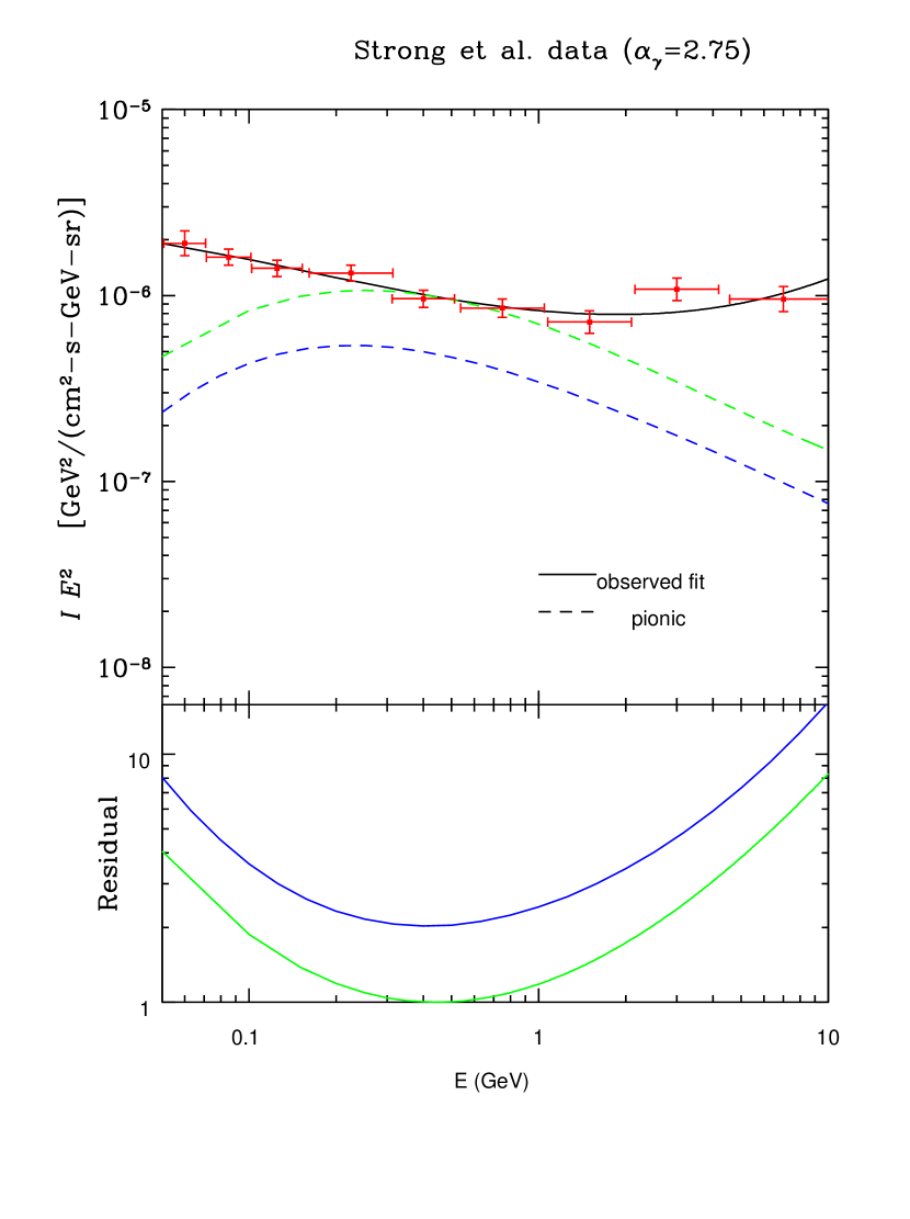
Figure 1: In the upper panel of this figure, we plot the pionic (dashed lines:green- maximized, blue- normalized to the Milky Way) EGRB spectrum, where decaying pions are of GCR origin, compared to the observed EGRB spectrum (solid line, fit to data); for purposes of illustration, we use the Strong, Moskalenko, & Reimer (2004) data points, which are given in red crosses. The bottom panel represents the residual function, that is, $\log[(IE^{2})_{\rm obs}/(IE^{2})_{\pi}]=\log(I_{\rm obs}/I_{\pi})$.

Once we obtain the spectrum we can then fit it with

$$\ln(I_{\gamma_{\pi}}E^{2})=-14.171-0.546\ln E-0.131(\ln E)^{2}+0.032(\ln E)^{3}$$ (27)

where $E$ is in GeV and $I$ is in $\rm photons\ cm^{-2}\ s^{-1}\ sr^{-1}\ {\rm GeV^{-1}}$. The free leading term in the above equation is set by requiring that $I_{\gamma_{\pi}}=I_{\gamma,\rm obs}$ at the energy $E=0.44$ GeV which maximizes pionic contribution by demanding that the pionic gamma-ray spectrum always stays below the observed one (since the feature of pionic peak is not observed). We also fit the Strong, Moskalenko, & Reimer (2004) data with

$$\ln(I_{\gamma,\rm obs}E^{2})=-14.003-0.144\ln E-0.097(\ln E)^{2}+0.017(\ln E)^{3}$$ (28)

in the same units.

By going through the procedure described in §3.1 (see Prodanović & Fields, 2004, for more detail) we can now obtain an upper limit to the fraction of pionic gamma-ray compared to the Strong, Moskalenko, & Reimer (2004) observed EGRB spectrum. This maximized pionic (green dashed line), as well as the observed, gamma-ray spectrum is presented in Fig. 1. We find the upper limit to pionic fraction to be $f_{\pi}(>0.1{\rm GeV})\equiv\int_{0.1}dE\,I_{\gamma_{\pi}}/\int_{0.1}dE\,I_{\gamma,\rm obs}=0.75$. We note in passing that a maximal pionic fraction as appears in Fig. 1 gives a poor fit at energies both above and below the matching near 0.4 GeV, suggesting the presence of other source mechanisms. This mismatch reflects a similar problem in the underlying Galactic $\gamma$-ray spectrum, and suggests that the pionic contribution to the EGRB is in fact sub-maximal.

Thus, the pionic gamma-ray flux above 0.1 GeV is $I_{\gamma_{\pi}}(>0.1\ {\rm GeV})=0.83\times 10^{-5}\rm cm^{-2}\ s^{-1}\ sr^{-1}$. From eq. (21) it now follows that the total flux is $I_{\gamma_{\pi}}(>0)=2.31\times 10^{-5}\rm cm^{-2}\ s^{-1}\ sr^{-1}$. As before, we can now use eq. (14) to find the GCR ${}^{6}{\rm Li}$ mole fraction

$$\left(\frac{Y_{\mbox{${}^{6}{\rm Li}$}}}{Y_{\mbox{${}^{6}{\rm Li}$}_{\odot}}}\right)_{\rm GCR}=\frac{I_{\gamma_{\pi}}(>0)}{9.06\times 10^{-5}\ \rm photons\ cm^{-2}\ s^{-1}\ sr^{-1}}=0.25$$ (29)

and thus, SFCR-produced ${}^{6}{\rm Li}$ can be at most (neglecting the ${}^{6}{\rm Li}$ depletion) the residual ${}^{6}{\rm Li}$

$$\left(\frac{Y_{\mbox{${}^{6}{\rm Li}$}}}{Y_{\mbox{${}^{6}{\rm Li}$}_{\odot}}}\right)_{\rm SFCR} = 1-\left(\frac{Y_{\mbox{${}^{6}{\rm Li}$}}}{Y_{\mbox{${}^{6}{\rm Li}$}_{\odot}}}\right)_{\rm GCR}$$

$$= 0.75$$

With the appropriate scaling between ${}^{7}{\rm Li}$ and ${}^{6}{\rm Li}$ as given in Table 1, we can then determine the total elemental ${\rm Li}=\mbox{${}^{7}{\rm Li}$}+\mbox{${}^{6}{\rm Li}$}$ abundance and compare it to the primordial values from (19) and (20):

$$\left(\frac{\rm Li}{\rm H}\right)_{\rm SFCR}=3.45\times 10^{-10}=0.90\left(\frac{\mbox{${}^{7}{\rm Li}$}}{\rm H}\right)_{\rm p,thy}=2.81\left(\frac{\mbox{${}^{7}{\rm Li}$}}{\rm H}\right)_{\rm p,obs}$$

So far we have been determining the maximized pionic fraction of the EGRB based only on the shape of the pionic spectrum. However, in the case of normal galaxies we have a better understanding of what that fraction should be. That is, we can normalize pionic spectrum to the one of the Milky Way, and then integrate over the redshift history of sources. Following Pavlidou & Fields (2002) (and references therein) we set up the normalization by requiring that $\int_{0.1\ \rm GeV}dEL_{\gamma_{\pi}}(z=0,E)=\int_{0.1\ \rm GeV}dEL_{\gamma_{\pi},\rm MW}(E)=2.85\times 10^{42}\ \rm s^{-1}$. With the analytic fit of the shape of the pionic spectrum from Pfrommer & Enßlin (2003) this now gives:

$$L_{\gamma_{\pi}}(z=0,E)=9.52\times 10^{44}\rm\ s^{-1}\ GeV^{-1}\left[\left(\frac{2\epsilon}{m_{\pi^{0}}}\right)^{\delta_{\gamma}}+\left(\frac{2\epsilon}{m_{\pi^{0}}}\right)^{-\delta_{\gamma}}\right]^{-\alpha_{\gamma}/\delta_{\gamma}}$$ (31)

where $\alpha_{\gamma}=2.75$ for GCR spectrum, and $\delta_{\gamma}=0.14\alpha_{\gamma}^{-1.6}+0.44$. Now we can use equation (26) to obtain the pionic spectrum which is plotted on the Fig. 1(blue dashed line).We use star formation rate $\psi_{\rm MW}=3.2M_{\odot}\ \rm yr^{-1}$ (McKee, 1989). Finally we find that in this case, when pionic spectrum is normalized to the Milky Way, the GCR ${}^{6}{\rm Li}$ mole fraction that accompanies it is

$$\left(\frac{Y_{\mbox{${}^{6}{\rm Li}$}}}{Y_{\mbox{${}^{6}{\rm Li}$}_{\odot}}}\right)_{\rm GCR}=0.14$$

which then gives $({\rm Li/H})_{\rm SFCR}=3.96\times 10^{-10}=1.03({\mbox{${}^{7}{\rm Li}$}}/{\rm H})_{\rm p,thy}=3.22(\mbox{${}^{7}{\rm Li}$}/{\rm H})_{\rm p,obs}$, which is of course a weaker limit than the maximal pionic case.

We thus see that in a completely model-independent analysis, current observations allow the possibility that SFCRs are quite a significant source of ${}^{6}{\rm Li}$ and of $\gamma$-rays. Indeed, we cannot exclude that SFCR-produced lithium can be a potentially large contaminant of the pre-Galactic Li component of halo stars, which would exacerbate the already troublesome disagreement with CMB-based estimates of primordial ${}^{7}{\rm Li}$. Consequently, we conclude that models for SFCR acceleration and propagation should include both $\gamma$-ray and ${}^{6}{\rm Li}$ production; and more constraints on SFCR, both theoretically (e.g., space and time histories) and observationally (e.g., EGRB and possibly diffuse synchrotron measurement), will clarify the picture we have sketched.

Note that had we also considered the possibility of depletion of ${}^{6}{\rm Li}$ , we would have found a greater ${}^{6}{\rm Li}$ residual, and thus had an even larger SFCR-produced component.

5 ${}^{6}{\rm Li}$ and Gamma-Rays From Cosmological Cosmic Rays

In this section we turn to the as-yet unobserved cosmological component of cosmic rays, and to the synthesis of lithium by SFCR. This lithium component would be the first made after big bang nucleosynthesis. Any Li which is produced this way prior to the most metal-poor halo stars would amount to a pre-Galactic Li enrichment and thus would be a non-primordial Li component, unaccompanied by beryllium and boron production. This structure-formation Li would be an additional “contaminant” to the usual components in halo stars, the ${}^{7}{\rm Li}$ abundance due to primordial nucleosynthesis, and the ${}^{6}{\rm Li}$ and ${}^{7}{\rm Li}$ contribution due to Galactic cosmic rays Ryan et al. (2000). Moreover, the pre-Galactic but non-primordial component would by itself be indistinguishable from the true primordial component, and thus would lead to an overestimate of the BBN ${}^{7}{\rm Li}$ production.

Our goal in this section is to exploit the $\gamma$-ray connection to constrain the structure-formation Li contamination. Unfortunately, we currently lack a detailed understanding of the amount and time-history of the structure formation cosmic rays (and resulting $\gamma$-rays and Li). Thus we will make the conservative assumption that all structure formation cosmic rays, and the resulting $\gamma$s and Li, are generated prior to any halo stars. Furthermore, we will assume that the pionic contribution to the EGRB is entirely due to structure formation cosmic rays. This allows us to relate observational limits on the pionic EGRB to pre-Galactic Li.

With this assumption and a SFCR composition $\Phi_{\alpha}^{\rm cr}/\Phi_{p}^{\rm cr}\approx y_{\alpha}^{\rm cr}=0.1$, we can now use the appropriate scaling factor from Table 1 to rewrite eq. (13)

$$I_{\gamma,\pi^{0}}(\epsilon>0,z) = \frac{\xi_{\gamma}\zeta_{\alpha}}{4\pi y_{\rm\alpha}^{\rm cr}y_{\rm\alpha}^{\rm ism}}\frac{\zeta\sigma_{\pi^{0}}}{\sigma_{\mbox{${}^{6}{\rm Li}$}}^{\alpha\alpha}}\left(\frac{\mbox{${}^{6}{\rm Li}$}}{\rm H}\right)n_{\rm b}c$$ (32)

$$= 1.86\times 10^{-5}\ \rm photons\ cm^{-2}\ s^{-1}\ sr^{-1}\ \left(\frac{\mbox{${}^{6}{\rm Li}$}}{\mbox{${}^{6}{\rm Li}$}_{\odot}}\right)$$ (33)

or

$$\left(\frac{\mbox{${}^{6}{\rm Li}$}}{\mbox{${}^{6}{\rm Li}$}_{\odot}}\right)=0.538\left(\frac{I_{\gamma,\pi^{0}}(>0)}{10^{-5}\ \rm cm^{-2}\ s^{-1}\ sr^{-1}}\right)$$ (34)

where we used the solar lithium mole fraction $Y(\mbox{${}^{6}{\rm Li}$})_{\odot}=1.09\times 10^{-10}$.

To set up an extreme upper limit on pre-Galactic SFCR ${}^{6}{\rm Li}$, we assume that the entire pionic extragalactic gamma-ray background came from SFCR-made pions, and was created prior to any halo star. As mentioned in the previous section, the method used in subtraction of the Galactic foreground is crucial for obtaining the EGRB spectrum. What is more, the EGRB spectrum is an important input parameter in the Prodanović & Fields (2004) analysis whose estimates of the maximal pionic gamma-ray flux we will use here. Our results for the SFCR lithium upper limits are collected in Table 2. The results depend on the choice of the EGRB spectrum as well as the redshift of origin of cosmic-rays according to the single-redshift approximation used by Prodanović & Fields (2004) to obtain the maximal pionic EGRB fraction. Note that we considered only the two most extreme redshifts to illustrate the results. In the Table 2, $z$ is the redshift, $I_{\gamma,\pi}(>0)$ is the upper limit for the pionic $\gamma$-ray intensity above 0 energy determined from (18) as explained in the previous section, $({\rm Li/H})_{\rm SFCR}^{\rm max}$ is the upper limit to total ($\mbox{${}^{6}{\rm Li}$}+\mbox{${}^{7}{\rm Li}$}$) lithium abundance that can be of SFCR origin, while ${\rm Li}_{p}^{\rm theo}$ and ${\rm Li}_{p}^{\rm obs}$ are the theoretical and observational primordial lithium abundances respectively as given in equations (20) and (19).

Notice that for the case of Keshet, Waxman, & Loeb (2003) EGRB, since a spectrum was unavailable, the procedure described in the section §3.1 for maximizing the pionic fraction of the EGRB could not be used. Thus, to place an upper limit on SFCR lithium we assumed that the entire EGRB can be attributed to decays of pions, that is, assume $I_{\gamma}=I_{\gamma,\pi^{0}}$. For the Sreekumar et al. (1998) and Strong, Moskalenko, & Reimer (2004) EGRB spectra, we use the upper limits to $I_{\gamma,\pi^{0}}$ obtained by Prodanović & Fields (2004). Once the $I_{\gamma,\pi^{0}}$ is set we can use (34) to find the SFCR ${}^{6}{\rm Li}$ upper limit.

To find the total halo star contribution we must also include ${}^{7}{\rm Li}$, which is in fact produced more than ${}^{6}{\rm Li}$ in $\alpha\alpha$ fusion: as seen in Table 1, ${\rm(^{7}Li/\mbox{${}^{6}{\rm Li}$})}_{\rm SFCR}=\langle\sigma_{{}^{7}Li}^{\alpha\alpha}\rangle/\langle\sigma_{\mbox{${}^{6}{\rm Li}$}}^{\alpha\alpha}\rangle\approx 2$. The total SFCR elemental Li production appears in Table 2, both in terms of the absolute Li/H abundance and its ratio to the different measures of primordial Li (§3.2).

Table 2: Upper limit on Li of SFCR origin

EGRB [$\rm cm^{-2}s^{-1}sr^{-1}$]	$z$	$I_{\gamma,\pi}(>0)$	$\rm(Li/H)_{SFCR}^{max}$	$\rm\frac{Li_{SFCR}^{max}}{Li_{p}^{theo}}$	$\rm\frac{Li_{SFCR}^{max}}{Li_{p}^{obs}}$	$f_{\pi}$
Sreekumar et al. (1998)	0	$8.78\times 10^{-6}$	$2.19\times 10^{-10}$	0.57	1.78	0.91
$I_{\gamma,\rm obs}(>0.1)=1.57\times 10^{-5}$	10	$1.22\times 10^{-4}$	$3.04\times 10^{-9}$	7.95	24.7	0.15
Strong et al. (2004)	0	$4.59\times 10^{-6}$	$1.14\times 10^{-10}$	0.30	0.93	1.29
$I_{\gamma,\rm obs}(>0.1)=1.11\times 10^{-5}$	10	$6.27\times 10^{-5}$	$1.56\times 10^{-9}$	4.09	12.69	0.21
Keshet et al. (2003)	0	$<6.5\times 10^{-6}$	$<1.62\times 10^{-10}$	0.42	1.32	2.86
$I_{\gamma,\rm obs}(>0.1)<0.5\times 10^{-5}$	10	$<4.03\times 10^{-5}$	$<1.00\times 10^{-9}$	2.63	8.16	0.46

From Table 2 we see that the maximal possible SFCR contribution to halo star lithium could be quite substantial. If the pre-Galactic SFCR component is dominantly produced at high redshift (i.e., as in the $z\sim 10$ results) then the maximum allowed Li production is can exceed the primordial Li production (however it is estimated), in some cases by a factor up to 25! The situation is somewhat better if the pre-Galactic SFCR production is at low redshift, but here it is hard to understand how this would predate the halo star component of our Galaxy. The high-redshift result is thus the more likely one, but also somewhat troubling in that the limit is not constraining. The indirect limits on SFCR Li in the previous section are somewhat stronger, but these also hold the door open for a significant level of pre-Galactic synthesis.

We caution that the lack of a strong constraint on SFCR Li production is not the same as positive evidence that the production was large. Recall that we have made several assumptions which purposely maximize the SFCR contribution; to the extent that these assumptions fail, the contribution falls, perhaps drastically. A more detailed theoretical and observational understanding of the SFCR history, and of the EGRB, will help to clarify this situation. Moreover, given that the halo star Li is already found to be below the CMB-based ${}^{7}{\rm Li}$ BBN results, we are already strongly biased to believe that the pre-Galactic SFCR component is not very large. Thus one might be tempted instead to go the other way and use Li abundances to constrain SFCR activity.

We thus now go the other way and use solar ${}^{6}{\rm Li}$ to constrain the SFCR $\gamma$-ray flux. Again, given our incomplete knowledge of SFCRs, we must adopt a simplifying assumption about the degree of ${}^{6}{\rm Li}$ production which is due to SFCR. To be conservative, we make the extreme assumption is that all of the solar ${}^{6}{\rm Li}$ is produced by SFCR, and thus find via eq. (32) that $\gamma$-flux is $I_{\gamma,\pi^{0}}(>0\rm\ GeV)>1.86\times 10^{-5}\ \rm photons\ cm^{-2}\ s^{-1}\ sr^{-1}$. From (18) we can determine $I_{\gamma,\pi^{0}}(>0.1\rm\ GeV)$ to be $0.23\times 10^{-5}<I_{\gamma,\pi^{0}}(>0.1\rm\ GeV)<1.43\times 10^{-5}\rm photons\ cm^{-2}\ s^{-1}\ sr^{-1}$ depending on the redshift of pionic $\gamma$-rays, which is below the observed level as determined by Sreekumar et al. (1998), and a factor of 2-14 lower than the prediction based on GCR. Thus, for a given observed intensity $I_{\gamma}^{\rm obs}(>\epsilon_{0})$ we can now use (18) to constraint the hadronic fraction of EGRB, that is, calculate $f_{\pi}(>\epsilon_{0},z)$ which is also presented in the Table 2.

However, since Li is being depleted, the use of the solar ${}^{6}{\rm Li}$ abundance does not give us the upper most limit to the required pionic gamma-ray flux $I_{\gamma,\pi^{0}}(>0)$. Thus, if one would to compensate for the depletion, the pionic fraction $f_{\pi}(>\epsilon_{0},z)$ would become even larger.

Indeed, this may suggest a solution to the EGRB overproduction by GCRs, seen in the previous section. If ${}^{6}{\rm Li}$ is mostly made by SFCRs, then the associated $\gamma$-ray production is in line with the observed background. In this case, ${}^{6}{\rm Li}$ would still be of cosmic-ray origin, but not dominated by GCR production. Such a scenario faces tests regarding ${}^{6}{\rm Li}$ and other LiBeB abundances and their Galactic evolution. A detailed discussion of this scenario will appear in a forthcoming study.

6 Discussion

The main result of this paper is to identify and quantify the tight connection between ${}^{6}{\rm Li}$ and the EGRB as measures of cosmic-ray history. Specifically, these two observables provide measures of average, gas-weighted cosmic-ray fluence. Moreover, the observables are complementary, in that ${}^{6}{\rm Li}$ samples local fluence, while the EGRB encodes the cosmic mean fluence.

We present scaling laws which relate ${}^{6}{\rm Li}$ and the EGRB intensity for different cosmic ray spectra appropriate for GCR and SFCR populations. Using these scalings, and assuming that our local ${}^{6}{\rm Li}$ measurements are typical, we can test the self-consistency of ${}^{6}{\rm Li}$ and EGRB observations in a relatively model-independent manner. We find that if SFCR dominate the pionic EGRB, then the associated ${}^{6}{\rm Li}$ production can be a significant and perhaps dominant contribution to the solar abundance. On the other hand, we find that if ${}^{6}{\rm Li}$ production is dominated by GCRs, then the associated $\gamma$-ray production is enormous, at least a factor of two above the observed intensity.

Furthermore, using the EGRB we use two different lines of argument to place an upper limit on the SFCR contribution to pre-Galactic lithium in halo stars. Such a component of lithium would be confused with the true primordial abundance and thus would exacerbate the existing deficit in halo star Li relative to the CMB-based expectations of BBN theory. Unfortunately, current EGRB data are such that our model-independent upper limit (which most assume, among other things, that all SFCRs are created prior to any halo stars) is very weak. In particular, we cannot exclude the possibility that a significant portion of pre-Galactic lithium is due to SFCRs. We thus find that the nucleosynthesis aspects of SFCRs are important and deserver further more detailed study.

A full understanding of the implications of the relationships among ${}^{6}{\rm Li}$, diffuse $\gamma$-rays, and cosmic ray populations thus awaits better observational constraints (both light elements and especially the EGRB) as well as a more detailed study of SFCRs. Having shown the importance of both the ${}^{6}{\rm Li}$ and $\gamma$-ray constraints, it is our hope that these observables will be calculated in models of galactic and structure formation cosmic rays, and that both ${}^{6}{\rm Li}$ and the EGRB are used in concert to constrain cosmic-ray interactions with diffuse matter. The results of these models will go far to address some of the questions which this study has raised.

Appendix A Notation and Normalization Conventions

The interactions of cosmic-ray species $i$ with target nucleus $j$ produces species $k$ at a rate per target particle of

$$\Gamma_{k}=\int_{E_{{\rm th},k}}dE\,\sigma_{ij\rightarrow k}(E)\phi_{i}\equiv\sigma_{ij\rightarrow k}\Phi_{i}$$ (A1)

Here $E$ is the cosmic-ray energy per nucleon, $\sigma_{ij\rightarrow k}$ is the energy-dependent production cross section, with threshold $E_{{\rm th},k}$, and $\phi_{i}$ is the cosmic-ray flux. The rate per unit volume for $i+j\rightarrow k$ is thus $q_{k}=\Gamma_{k}n_{j}$.

Note that the flux in eq. (A1) is position- and time-dependent. To isolate this dependence, it is useful to define a total, energy-integrated, flux

$$\Phi_{i}=\int_{E_{\rm th,min}}dE\,\phi_{i}$$ (A2)

where we choose the lower integration limit to always be the minimum threshold $E_{\rm th,min}$ for all reactions considered; in our case this is the $\alpha+\alpha\rightarrow\mbox{${}^{7}{\rm Li}$}$ threshold of $8.7$ MeV/nucleon. From eqs. (A1) and (A2) it follows that

$$\sigma_{ij\rightarrow k}=\Gamma_{k}/\Phi_{i}$$ (A3)

represents a flux-averaged cross section. Also note that if the spectral shape of $\phi_{i}$ is constant (as we always assume), then so is $\sigma_{ij\rightarrow k}$, and the flux $\Phi_{i}$ contains all of the time and space variation of $\Gamma_{k}$.

Finally, two conventions are useful for quantifying abundances. Species $i$, with number density $n_{i}$, has a “mole fraction” (or baryon fraction) $Y_{i}=n_{i}/n_{\rm b}$. It is also convenient to introduce the “hydrogen ratio” $y_{i}=n_{i}/n_{\rm H}=Y_{i}/Y_{\rm H}$.

Appendix B Cosmic Gamma-Radiation Transfer

The expression for $\gamma$-ray intensity in a Friedmann universe is well-known (Stecker, 1969), but usually expressed in redshift space. For our purposes, the result expressed in the time domain is critical, and indeed is more fundamental, so we give a derivation based on the Boltzmann equation. For this section we adopt units in which $c=1$.

The differential photon (number) intensity $I$ is directly related via

$$I(\vec{p},\vec{x},t)=p^{2}f(\vec{p},\vec{x},t)$$ (B1)

to the $\gamma$-ray distribution function $f(\vec{p},\vec{x},t)=d^{3}N/d^{3}\vec{p}d^{3}\vec{x}$ Here $\vec{p}$ and $\vec{x}$, as well as the volume elements, are physical quantities (and thus subject to change with cosmic expansion). The distribution function is related to the photon sources via the relativistic Boltzmann equation

$$p^{\mu}\partial_{\mu}f-\Gamma_{\mu}^{\alpha\beta}p^{\alpha}p^{\beta}f=E\frac{dq}{d^{3}\vec{p}}$$ (B2)

where gravitational effects enter through the Affine connection $\Gamma$, where $E=p=|\vec{p}|$, and where the source function (number of photons created per unit volume per unit time) is $q$.

For an isotropic FRW universe we have $f=f(E,t)$, and thus

$$\partial_{t}f-\frac{\dot{a}}{a}E\partial_{E}f=\frac{q(E)}{4\pi E^{2}}$$ (B3)

where $q(E)=dq/dE$ and where we neglect photon scattering and absorption.

We now note that a given photon’s energy $E$ drops due to redshifting as $a^{-1}$. It is thus useful to define a comoving energy $\epsilon=aE$; with $a(t_{0})=1$, we see that $\epsilon$ is also the present-day (observed) photon energy. Changing variables from $f(E,t)$ to $f(\epsilon,t)$, and similarly for $q$, the energy-dependent $\partial_{\epsilon}$ term drops out; this is physically reasonable since we do not allow for scattering processes, and thus a photon’s energy can only change due to redshifting. We then have

$$\partial_{t}f=a^{2}\frac{q(\epsilon/a)}{4\pi\epsilon^{2}}$$ (B4)

which, for any fixed comoving energy $\epsilon$, integrates to

$$f(\epsilon,t)=\frac{1}{4\pi\epsilon^{2}}\int_{0}^{t}dt^{\prime}\ a^{2}\ q(\epsilon/a)$$ (B5)

Equation (B1) then gives the intensity

$$I(\epsilon,t)=\frac{1}{4\pi a(t)^{2}}\int_{0}^{t}dt^{\prime}\ \frac{1}{a(t^{\prime})}q_{\rm com}[\epsilon/a(t^{\prime})]$$ (B6)

where $q_{\rm com}=a^{3}q$ is the comoving source rate. Equation (B6) is the usual expression (which is often then expressed in terms of an integral over redshift). Finally, if we integrate over the entire energy spectrum, and evaluate at the present epoch $t_{0}$ (when $a_{0}=1$), we have

$$I(>0,t_{0})=\int_{0}^{\infty}d\epsilon\,I(\epsilon,t_{0})=\frac{1}{4\pi}\int_{0}^{t_{0}}dt^{\prime}\ q_{\rm com}(>0)$$ (B7)

where $q_{\rm com}(>0)=\int_{0}^{\infty}du\ q(u)$ is the total source rate, integrated over rest-frame energy.

We see from eq. (B7) that the energy-integrated intensity is the same as one would find from uniform sources in a non-expanding universe (which have been “switched on” for a duration $t$). This result is physically sensible, because the two effects of cosmic expansion are to introduce a particle horizon and redshifting. The energy integration removes the effect of redshifting, so that the only effect is that of the particle horizon, which acts to set the integration timescale.

References

- Anders & Grevesse (1989) Anders, E. & Grevesse, N. 1989, Geochim. Cosmochim. Acta, 53, 197
- Blasi (2004) Blasi, P. 2004, Astroparticle Physics, 21, 4
- Brooks et al. (2002) Brooks, A. M., Venn, K. A., Lambert, D. L., Lemke, M., Cunha, K., & Smith, V. V. 2002, ApJ, 573, 584
- Cassé, Vangioni-Flam, & Audouze (2001) Cassé, M., Vangioni-Flam, E., & Audouze, J. 2001, in Cosmic Evolution, ed. E. Vangioni-Flam, R. Ferlet, and M. Lemoine, (World Scientific: New Jersey), 107
- Cole et al. (2001) Cole, S., et al. 2001, MNRAS, 326, 255
- Cyburt, Ellis, Fields, & Olive (2003) Cyburt, R. H., Ellis, J., Fields, B. D., & Olive, K. A. 2003, Phys. Rev. D, 67, 103521
- Cyburt, Fields, & Olive (2003) Cyburt, R. H., Fields, B. D., & Olive, K. A. 2003, Physics Letters B, 567, 227
- Cyburt, Fields, & Olive (2003) Cyburt, R. H.& Fields, B. D. 2004, Phys. Rev. D in press (astro-ph/312629)
- Dermer (1986) Dermer, C. D. 1986, A&A, 157, 223
- Dimopoulos, Esmailzadeh, Starkman, & Hall (1988) Dimopoulos, S., Esmailzadeh, R., Starkman, G. D., & Hall, L. J. 1988, ApJ, 330, 545
- Fichtel, Kniffen, & Hartman (1973) Fichtel, C. E., Kniffen, D. A., & Hartman, R. C. 1973, ApJ, 186, L99
- Fields (1999) Fields, B. D. 1999, ApJ, 515, 603
- Fields & Olive (1999a) Fields, B. D. & Olive, K. A. 1999a, ApJ, 516, 797
- Fields & Olive (1999b) Fields, B. D. & Olive, K. A. 1999b, New Astronomy, 4, 255
- Gabici & Blasi (2003) Gabici, S. & Blasi, P. 2003, Astroparticle Physics, 19, 679
- Gehrels & Michelson (1999) Gehrels, N. & Michelson, P. 1999, Astroparticle Physics, 11, 277
- Hunter et al. (1997) Hunter, S. D., et al. 1997, ApJ, 481, 205
- Jedamzik (2000) Jedamzik, K. 2000, Physical Review Letters, 84, 3248
- Jones & Ellison (1991) Jones, F. C. & Ellison, D. C. 1991, Space Science Reviews, 58, 259
- Kang, Jones, & Gieseler (2002) Kang, H., Jones, T. W., & Gieseler, U. D. J. 2002, ApJ, 579, 337
- Keshet, Waxman, & Loeb (2003) Keshet, U., Waxman, E., & Loeb, A. 2003, ApJ submitted (astro-ph/0306442)
- Keshet et al. (2003) Keshet, U., Waxman, E., Loeb, A., Springel, V., & Hernquist, L. 2003, ApJ, 585, 128
- Kawasaki, Kohri, & Moroi (2001) Kawasaki, M., Kohri, K., & Moroi, T. 2001, Phys. Rev. D, 63, 103502
- Loeb & Waxman (2000) Loeb, A. & Waxman, E. 2000, Nature, 405, 156
- McKee (1989) McKee, C. F. 1989, ApJ, 345, 782
- Mercer et al. (2001) Mercer, D. J. et al. 2001, Phys. Rev. C, 63, 65805
- Miniati (2002) Miniati, F. 2002, MNRAS, 337, 199
- Miniati et al. (2000) Miniati, F., Ryu, D., Kang, H., Jones, T. W., Cen, R., & Ostriker, J. P. 2000, ApJ, 542, 608
- Montmerle (1977a) Montmerle, T. 1977, ApJ, 216, 177
- Montmerle (1977b) Montmerle, T. 1977, ApJ, 216, 620
- Montmerle (1977c) Montmerle, T. 1977, ApJ, 217, 878
- Mukherjee & Chiang (1999) Mukherjee, R. & Chiang, J. 1999, Astroparticle Physics, 11, 213
- Pavlidou & Fields (2001) Pavlidou, V. & Fields, B. D. 2001, ApJ, 558, 63
- Pavlidou & Fields (2002) Pavlidou, V. & Fields, B. D. 2002, ApJ, 575, L5
- Pfrommer & Enßlin (2003) Pfrommer, C. & Enßlin, T. A. 2003, A&A, 407, L73
- Prodanović & Fields (2004) Prodanović, T., & Fields, B. D. 2004, APh submitted (astro-ph/0403300)
- Ramaty, Scully, Lingenfelter, & Kozlovsky (2000) Ramaty, R., Scully, S. T., Lingenfelter, R. E., & Kozlovsky, B. 2000, ApJ, 534, 747
- Read & Viola (1984) Read, S.M., & Viola, V.E. 1984, Atomic Data Nucl. Data 31, 359
- Romano, Matteucci, Ventura, & D’Antona (2001) Romano, D., Matteucci, F., Ventura, P., & D’Antona, F. 2001, A&A, 374, 646
- Ryan et al. (2000) Ryan, S. G., Beers, T. C., Olive, K. A., Fields, B. D., & Norris, J. E. 2000, ApJ, 530, L57
- Ryu, Kang, Hallman, & Jones (2003) Ryu, D., Kang, H., Hallman, E., & Jones, T. W. 2003, ApJ, 593, 599
- Spergel et al. (2003) Spergel, D. N., et al. 2003, ApJS, 148, 175
- Sreekumar et al. (1998) Sreekumar, P. et al. 1998, ApJ, 494, 523
- Stecker (1969) Stecker, F. W. 1969, ApJ, 157, 507
- Stecker & Salamon (1996) Stecker, F. W. & Salamon, M. H. 1996, ApJ, 464, 600
- Steigman & Walker (1992) Steigman, G. & Walker, T. P. 1992, ApJ, 385, L13
- Strong, Moskalenko, & Reimer (2004) Strong, A. W., Moskalenko, I. V., & Reimer, O. 2004, ApJ in press (astro-ph/0405441)
- Suzuki & Inoue (2002) Suzuki, T. K. & Inoue, S. 2002, ApJ, 573, 168
- Travaglio et al. (2001) Travaglio, C., Randich, S., Galli, D., Lattanzio, J., Elliott, L. M., Forestini, M., & Ferrini, F. 2001, ApJ, 559, 909
- Vangioni-Flam et al. (1999) Vangioni-Flam, E., Casse, M., Cayrel, R., Audouze, J., Spite, M., & Spite, F. 1999, New Astronomy, 4, 245
- Vangioni-Flam & Cassé (2001) Vangioni-Flam, E. & Cassé, M. 2001, New Astronomy Review, 45, 583
- Woosley, Hartmann, Hoffman, & Haxton (1990) Woosley, S. E., Hartmann, D. H., Hoffman, R. D., & Haxton, W. C. 1990, ApJ, 356, 272
- Yoshida, Terasawa, Kajino, & Sumiyoshi (2004) Yoshida, T., Terasawa, M., Kajino, T., & Sumiyoshi, K. 2004, ApJ, 600, 204
- Zweibel (2003) Zweibel, E. G. 2003, ApJ, 587, 625