An all-sky optical catalogue of radio / X-ray sources

We present an all-sky catalogue that aligns and overlays the ROSAT HRI, RASS, PSPC and WGA X-ray catalogues and the NVSS, FIRST and SUMSS radio catalogues onto the optical APM and USNO-A catalogues. Objects presented are those APM/USNO-A optical objects which are calculated with $\geq 40$% confidence to be associated with radio/X-ray detections, or which are identified as known QSOs, AGN or BL Lacs, totalling 501,761 objects in all, including 48,285 QSOs and 21,498 double radio lobe detections. For each radio/X-ray associated optical object we display the calculated percentage probabilities of its being a QSO, galaxy, star, or erroneous radio/X-ray association, plus any identification from the literature. The catalogue includes 86,009 objects which were not previously identified and which we list as being 40% to $>99$% likely to be a QSO. As a byproduct of the construction of this catalogue, we are able to list comprehensive ROSAT field shifts as determined by our whole-sky likelihood algorithm, and also plate-by-plate photometric recalibration of the complete APM and USNO-A2.0 optical catalogues, significantly improving accuracy for objects of $>15$ mag. The catalogue is available wholly and in subsets at http://quasars.org/qorg-data.htm .

1 Introduction

In recent years a number of good-resolution radio and X-ray surveys have been completed and the full data published. One major goal of such surveys is that the radio/X-ray detections should be associated with optical objects to further their classification and to find new examples of emission phenomena. Previous such efforts generally treat just one radio/X-ray survey per paper, and use matching criteria particular to that paper; see notably APM Optical Counterparts to FIRST Radio Sources (MWHB: McMahon et al. 2002) and the Hamburg/RASS Catalogue of Optical Identifications (HRC: Bade et al. 1998) which has multiple optical identifications per X-ray detection. It is desirable for there to be a single unified catalogue which combines and overlays all these good-resolution radio/X-ray surveys onto the optical background using a uniform optimized matching algorithm. This paper presents such a catalogue: the ‘Quasars.org’ all-sky optical catalogue of radio/X-ray sources, obtainable from http://quasars.org/qorg-data.htm. The name refers to the website used as a repository during this catalogue’s development. We refer to our catalogue as ‘QORG’ throughout the rest of this paper.

The task of combining all these data was a complicated one, and our general approach was to start with no preconceptions but to let the data be our guide in evolving the best techniques. Iteration was commonly used to find stable results for data merging and calibration tasks. Extensive testing against well-understood control data allowed us to develop heuristic solutions for ROSAT field shifting and double radio lobe identification. We developed a whole-sky based method of calculating likelihood-of-association which causally ties optical objects to radio/X-ray sources. These likelihoods are written into our catalogue as percentage odds that each associated optical object is in turn a QSO, galaxy, star, or erroneous radio/X-ray association. Objects presented are APM/USNO-A optical objects calculated with $\geq 40$% confidence to be associated with radio/X-ray detections, or which are identified as known QSOs, AGN or BL Lacs; the 40% threshold is an arbitrary choice, but ensures that the catalogue contains only interesting or potentially interesting objects. These optical objects total 501,761 in all, including 119,816 objects bearing identifications from the literature and 86,009 objects not hitherto identified which we list as being 40% to $>99$% likely to be a QSO.

This paper is divided into sections as follows: (2) an account of all the source catalogues used in this compilation; (3) a brief summary of our primary likelihood algorithm, ROSAT field shifts, and technique used to identify double radio lobes; (4) a description of our main catalogue. The electronic paper includes an appendix detailing, at some length, our methods and the issues encountered during the construction of the catalogue. Its sections are: (1) issues in the construction and recalibration of the merged optical catalogue used for the background, and its attributes; (2) description of the likelihood calculations used to causally associate optical objects with radio/X-ray sources; (3) issues in overlaying the X-ray detections onto the optical background, notably the field shifts required; (4) issues in overlaying the radio detections onto the optical background and identifying double radio lobes; (5) issues in matching identification catalogues to the optical background; (6) attributes and analysis of the resulting Quasars.org catalogue.

2 The Source Catalogues

Source catalogues included are categorized as optical, radio, X-ray, or identification catalogues.

2.1 Optical Surveys

The whole-sky optical background represents by far the largest data pool to be incorporated, although only those optical objects which are associated with radio/X-ray detections, or are known quasars, are included in the final QORG catalogue. This project commenced in 1999 and we used the optical data available at that time to compile our own in-house whole-sky optical catalogue. Our main source was the complete set of the Cambridge Automatic Plate Measuring machine (APM: McMahon and Irwin 1992) scans of 1906 plates on the North and South Galactic caps, consisting of 896 first-epoch National Geographic-Palomar Observatory Sky Survey (POSS-I) $E$ and $O$ plates centred on equatorial declinations $0\degr$ to $+90\degr$, and 1010 second-epoch UK Schmidt Telescope sky survey (UKST) ESO-R and SRC-J plates centred on declinations $-85\degr$ to $0\degr$; these yielded about 270,000,000 sources in one or more colours. We also include the United States Naval Observatory whole-sky catalogues (USNO-A) which used the Precision Measuring Machine (PMM) to read sources from the POSS-I and UKST plates. The USNO-A catalogues are not as deep as the APM so are treated as supplementary data, but only USNO-A covers the Galactic plane area. The earlier USNO-A1.0 (Monet et al. 1998) lists 488,006,860 sources in both red and blue, with POSS-I plates used for field centres down to declination $-30\degr$, and UKST plates below that. USNO-A2.0 (Monet et al. 1998) lists 526,280,881 sources in both red and blue; the additional sources were a result of a re-reduction of the PMM scans and switching from POSS-I plates to the deeper UKST plates for field centres with declinations of $-20\degr$ to $-30\degr$.

2.2 Radio Surveys

The largest radio survey is the NRAO VLA Sky Survey (NVSS: Condon et al. 1998) catalogue 40 (2002), which is a 1.4-GHz all-sky survey down to a declination of $-40\degr$, with a source detection threshold of 2.5 mJy and positional accuracy ranging from $<1$ arcsec for the strongest sources to 7 arcsec at the faint limit. A second radio survey is the Faint Images of the Radio Sky at Twenty-cm survey (FIRST: White et al. 1997) which has recently (April 2003) been completed; this is a 1.4-GHz survey of 9033 square degrees of primarily the north Galactic cap, with a source detection threshold of 1 mJy and a positional accuracy within 1 arcsec. The FIRST survey overlaps the NVSS in its surveyed area but is deeper and has better resolution. The part of the sky not covered by the NVSS is currently being surveyed at 843 MHz by the Sydney University Molonglo Sky Survey (SUMSS: Mauch et al. 2003, Oct 27 2003 release) to a comparable depth and resolution; this survey is at this time about 70 per cent complete so some of the sky below declination $-40\degr$ is as yet without radio coverage to this resolution, but the total sky coverage of these three radio surveys exceeds 95%.

2.3 X-ray surveys

The best-resolution X-ray surveys up to the end of the last decade all originate from ROSAT (ROentgen SATellite), which was operational from 1990 to 1999; its extragalactic and Galactic surveys are available in 4 primary catalogues. The ROSAT All-Sky Survey (RASS / revision 1RXS) is derived from the all-sky survey performed during the first half year of the ROSAT mission in 1990/91, and is available as two separate sub-catalogues: the Bright Source Catalogue (RASS-BSC: Voges et al. 1999a) containing 18,806 sources, and the Faint Source Catalogue (RASS-FSC: Voges et al. 2000) containing 105,924 sources. The RASS has a sky coverage of 92%, with a nominal positional accuracy of 30 arcsec. Secondly, the ROSAT Source Catalogue of Pointed Observations with the High Resolution Imager (HRI / 1RXH: Voges et al. 1999b) final release 1.3.0 (2001) has 131,902 sources from 5393 sequences representing a sky coverage of 1.94% with nominal positional accuracy of 5 arcsec. Third is the Second ROSAT Source Catalogue of Pointed Observations with the Position Sensitive Proportional Counter (PSPC / 2RXP: Voges et al. 1999b) final release 2.1.0 (2001) with 116,259 sources from 5182 sequences, representing a sky coverage of 17.3% with a nominal positional accuracy of 25 arcsec. We include with this the supplementary PSPC with Boron Filter catalogue (PSPCF: same attributions as PSPC) release 2.0.0 (2001), with 2526 sources from 258 sequences representing a sky coverage of 0.15%. Last is the WGA Catalogue of ROSAT Point Sources (WGA: White, Giommi & Angelini 1994) final release (August 2000) with 115,962 sources from 4160 sequences, which covers the same observational data as 2RXP but was originally released earlier and uses different data reduction algorithms. We use the WGA catalogue in recognition of the role it has played in research; it does include a few early sequences absent from the PSPC catalogue.

2.4 Identification catalogues

The fullest description of any radio/X-ray emitting object in the QORG catalogue is given when it is possible to identify it as a known QSO, AGN, BL Lac, galaxy or star. The following are the source catalogues for these types of objects which are used in the present task; web sites describing many of these are listed in the online data for the catalogue (http://quasars.org/ReadMe.txt)

The primary catalogue used for identification of QSOs, AGN and BL Lacs is the Catalogue of Quasars and Active Nuclei, 11th edition (Veron: Véron-Cetty & Véron 2003) which identifies 64,866 such objects, and uses an absolute-magnitude threshold to differentiate a QSO classification from an AGN classification, to which we adhere. We have added supplementary positional and name information from the large recent releases of the Sloan Digital Sky Survey (SDSS: Abazajian et al. 2003) and the 2dF QSO Redshift Survey (2QZ: Croom et al. 2003). We have also added 52 extra QSO identifications from the NASA/IPAC Extragalactic Database (NED) as those were found to have radio/X-ray associations, and 11 extra QSOs from the SDSS quasar catalog 2nd edition (Schneider et al, 2003) which made a supplementary release based on re-inspection of the SDSS spectra too late for inclusion in the Veron catalogue. However, we make use of only those objects for which we have an optical counterpart; in total this gives 48,285 QSOs, 14,633 AGN and 841 BL Lacs.

A measured redshift is required for identification as a QSO, but galaxies can reasonably be identified by visual morphology, although spectroscopy remains decisive. The primary catalogue used for identification of galaxies is the Principal Galaxy Catalogue (PGC) which is extracted from the Lyon-Meudon Extragalactic Database (LEDA: Paturel, Bottinelli, Gouguenheim 1995); our copy from September 2000 (courtesy of G. Paturel) contains 1,088,795 galaxies. We also use five redshift surveys which make galaxy identifications over a large sky area: the SDSS, the CfA Redshift Catalogue (CFA: Huchra et al. 1999, April 2003 edition), the IRAS PSCz Redshift Survey (PSCz: Saunders et al. 2000), the 2dF Galaxy Redshift Survey (2dFGRS: Colless et al. 2001) and the 6dF Galaxy Redshift Survey Early Data Release (6dFGS: Wakamatsu et al. 2002). Some extra identifications are sourced from the catalogue of Arcsecond Positions of UGC Galaxies (Cotton & Condon 1999), the 2QZ, the online 3CRR catalogue at http://www.3crr.dyndns.org/ (3CRR: Laing, Riley & Longair 1983), the Updated Zwicky Catalog (Zwicky: Falco et al. 1999) and the Redshift- Distance Survey of Nearby Early-Type Galaxies (ENEAR: Wegner et al. 2003). To summarize, for galaxies not classified as AGN, we utilize only those for which we have an optical object associated with a radio/X-ray detection; these total 49,743 galaxies. Note that some large galaxies known to be radio/X-ray emitters are missing from our catalogue because of astrometric mismatches between the available isophotally-bounded optical signatures and the radio/X-ray source locations.

The remaining possibility is that objects are identified with stars. This has been somewhat problematic, in that until recently stellar identifications were not often compiled, as they represented the detritus of QSO or galaxy surveys. Since radio/X-ray emitting objects are rarely stars, if such an object displayed a star-like spectrum it may have served only to keep it classified as an ‘unknown’ object. Large star catalogues such as Tycho (Hog et al. 2000) are actually just point source catalogues which do not make genuine stellar identification, and historic star catalogues are too astrometrically imprecise for unambiguous computerised matching, which we find to require astrometric precision of 15 arcsec or better. Recently, however, catalogues of stars of specific types such as white dwarfs have been released to the required astrometric precision, and large surveys like SDSS and 2dFGRS have published their star identifications; thus in the last few years the availability of suitable stellar data has greatly improved. We have used the following star catalogues for stellar identification: the Atlas of Cataclysmic Variables (CV: Downes et al. 2001), Spectroscopically Identified White Dwarfs (WD: McCook & Sion 1999), the General Catalogue of Variable Stars (Vol 1) with Improved Coordinates (GCVS: Samus et al. 2002), the revised New Luyten Two- Tenths catalogue of high proper-motion stars (NLTT: Salim & Gould 2003), stars from the Large Bright Quasar Survey (LBQS: Hewett et al. 1995) received courtesy of Paul Hewett, stars from the Las Campanas Redshift Survey (Shectman et al. 1996), and star identifications from the galaxy and QSO surveys listed above. We have also included the Tycho survey, as its objects are bright and very likely to be stars, and the Henry Draper Extension Charts (HDx: Nesterov et al. 1995) even though their stars are not confirmed spectroscopically. We have obtained names of bright stars from the Bright Star Catalogue, 5th Revised Ed. (Yale: Hoffleit & Warren 1991) and the Common Name Cross Index (Smith W.B. 1996). In the end we utilize only those stars for which we have an optical object associated with a radio/X-ray detection; these total 6314 stars.

3 All-Sky Based Likelihood Calculations and Matching Techniques

We give here a brief summary of the methods we used to relate optical objects to radio/X-ray sources, and to identify double radio lobes. An appendix that gives full details of our methods, together with supporting tabulated data, can be found in the electronic version of this paper.

Our primary algorithm to calculate the likelihood of association between optical and radio/X-ray sources is based on identifying classes of optical objects which tend to be astrometrically co-positioned with radio/X-ray sources, and assessing the significance of the relationship by comparison with whole-sky background averages. For example, if a class of optical object is found near NVSS sources at twice the areal density that it has on average in the background, then we say that the chance of association of those objects near the NVSS sources is 50%, as we expect half of the apparent associations to be chance superpositions of background objects. We define these optical object classes using four parameters: astrometric offset from the radio/X-ray source, photometric $(B-R)$ colour, APM psf classification, and local sky object density, binning these to provide large populations in each class and so minimize small-number fluctuations.

To improve the uniformity of our optical object classes we found it necessary to recalibrate the source data. The APM plate depths were photometrically recalibrated by matching stars on overlapping plate margins; this was done separately for red and blue plates. USNO-A photometry, which usually shows large zero-point offsets, was recalibrated into the APM standard using matched stars. These photometric recalibrations improve our $(B-R)$ colour data. The ROSAT source positions were recalibrated by using our likelihood algorithm to provide an optimal astrometric solution for each sequence; these typically involved shifts of 1-10 arcsec on the sky. These astrometric recalibrations improve our accuracy in gauging positional offset between individual optical objects and X-ray sources. As our recalibrations are potentially useful for others, we provide them on-line: the APM/USNO-A2.0 recalibration is listed plate-by-plate at http://quasars.org/docs/QORG-APM-USNO-calibration.txt, and the ROSAT field shifts are listed at http://quasars.org/docs/HRI-fields.txt for the HRI catalogue, and similarly for the RASS, PSPC and WGA input catalogues.

Table 1: Radio/X-ray Associations presented in the QORG catalogue.

Source catalogue	No. astrometrically	No. core	No. double
	unique sources	detections	lobes
		in QORG	in QORG
FIRST	781667	155132	11512
NVSS	1810664	242851	8323
SUMSS	165531	31156	1663
HRI	56398	12733
RASS	124730	30521
PSPC	102005	29472
WGA	88578	18712

As our aim was to derive maximum value from the source catalogues, we have also endeavoured to identify double radio lobes from the radio data. As QORG is an optical catalogue, we are interested only in those double lobes for which we have an optical centroid. We used a heuristic algorithm to identify these lobes, consisting of firstly enumerating the likely lobe population inherent within the radio data, then using a number of distinct rules to estimate the likelihood of a given radio-optical-radio configuration being a member of that lobe population. The details are given in the appendix. Table 1 summarizes the numbers of associations presented in QORG from each source catalogue.

4 The Optical Catalogue of Radio/X-ray Sources

The catalogue is available from the catalogue home page at http://quasars.org/qorg-data.htm, and is written as one line per optical object. The catalogue presents unique ‘best’ associations, so optical objects and radio/X-ray sources are not duplicated across lines; this keeps the presentation simple and plain. The full catalogue is in the ‘Master.txt’ file (21Mb zipped) which provides particulars of all 501,761 objects including data contributing to the likelihood calculations and double lobe declarations. A condensed version, ‘Free-Lunch.txt’, is also provided; this displays no more than 2 associations per object and omits supporting data. Also available are two subsets, ‘Known-Objects.txt’, which displays only the 119,816 objects from our catalogue which are identified from the literature, and ‘Quasar-Candidates.txt’ which displays the 86,009 objects from our catalogue not hitherto identified which we list as being 40% to $>99$% likely to be a QSO.

Table 2: Sample lines from the QORG catalogue (‘Free-Lunch’ variant)

J2000 location	type	$R$, $B$ (mag)	ct	psf	name	type percentages				$z$	radio/X-ray source 1	flux
(1)	(2)	(3)   (4)	(5)	(6)	(7)	(8)	(9)	(10)	(11)	(12)	(13)	(14)
040904.9-364744	GR	14.3 14.2		2 2	PGC 632512	0	98	0	2		NVSS J040904.8-364745	113
040905.0-053236	RX	19.1 20.3		1 1		12	74	0	14		NVSS J040904.6-053234	4
040905.2-283859	R	19.7 20.6		1 2		21	56	3	20		NVSS J040905.3-283859	4
040905.3+153056	R	16.9 21.2	p	n -		2	80	2	16		NVSS J040905.2+153051	3
040905.4-092350	R	17.2 19.4	p	2 1		2	89	0	9		NVSS J040905.4-092353	16
040905.8-123849	QR	18.0 18.4	p	- -	PKS0406-127	97	1	0	2	1.563	NVSS J040905.7-123847	450
040906.2-651733	R	15.0 15.1		- -		63	20	3	14		SUMSJ040905.3-651729	27
040906.2-041022	A	18.5 19.9	p	1 1	SDSSJ04-041					0.133
040906.3-760006	R	13.0 13.6		- -		2	46	15	37		SUMSJ040906.3-760006	6
040906.5-051054	Q	19.7 20.3		- -	SDSSJ04-051					1.556
040906.6-760534	R	18.6 19.8		1 1		3	63	0	34		SUMSJ040906.7-760532	6
040906.6+122356	X	20.2(20.0)	p	2 x		0	57	3	40		2RXP J040906.9+122353	6
040906.6+290944	SX	10.6   0	p	n n	HD281690	0	6	64	30		1RXS J040906.6+290943	92
040906.7-504531	R	18.7 21.6		2 1		2	92	0	6		SUMSJ040906.5-504528	18
040906.7-175710	QRX	19.1 20.6		- -	PKS 0406-18	64	6	4	26	0.722	NVSS J040906.6-175709	999
040906.8-681946	2	11.7 11.5		- -		2	19	51	28		SUMSJ040900.6-682023	36
040906.8-011844	R	19.0 21.3	p	1 -		12	67	0	21		NVSS J040906.7-011845	6
040907.3-043235	Q	19.1 19.8	p	- -	SDSSJ04-043					0.802
040907.6-304915	R	20.6(22.5)		- x		4	47	9	40		NVSS J040907.7-304916	2
040908.0-695738	X	18.8 21.5		n n		18	56	4	22		1RXS J040907.9-695735	71

Table 2 displays some sample lines of the QORG catalogue, using the Free-Lunch version (which is easily tabulated while showing the salient points of the similarly-structured main Master catalogue). ‘ReadMe’ files are provided on-line which give full file layouts, field definitions and supporting information for all catalogues; we only give an overview here. Column 1 displays the optical coordinates (epoch J2000) which doubles as the IAU-recommended name of the object, e.g., QORG J040904.9-364744. Column 2 summarizes any associations with, and identification of, the optical object: R=radio source, X=X-ray source, 2=double lobe declaration, Q=known quasar, A=AGN, G=galaxy, S=star, B=BL Lac object. Columns 3 and 4 give the red and blue magnitudes respectively, and column 5 states if those magnitudes are POSS-I (=’p’) or UKST photometry, plus flagging any nominal variability or proper motion. Column 6 gives the point spread function (psf) classification of the two optical observations, taken largely from the APM: ’-’=stellar, ’1’=fuzzy, ’2’=extended, ’n’=no psf and ’x’=object not seen in this colour. Column 7 gives the name of the object, where it is identified from the literature (abbreviated here for space reasons). Columns 8-11 give the calculated probability that the radio/X-ray associated object is turn a QSO, galaxy, star, or erroneous radio/X-ray association; this is discussed further in the next paragraph. Column 12 gives the redshift, if known. Column 13 gives the radio/X-ray source name for a declared association, and column 14 gives the flux in mJy for a radio association, or the count rate in counts/hour for a ROSAT X-ray association. A few of these objects are, in the Free-Lunch catalogue, listed also with a second radio/X-ray association which here is not shown for space reasons. The Master catalogue, which we expect will be of most general interest, lists up to six associations for each optical object, together with particulars of any double radio lobe found for it, supporting information which enables reconstitution of the likelihood calculation for that object, and references to the source catalogues for identified objects. Fig. 1 is a whole-sky optical density map of all 501,761 objects presented in the catalogue.

In the catalogue we display, for each radio/X-ray associated optical object, the calculated probabilities that it is a QSO (including BL Lacs), galaxy or star. We accumulated the data for these computations from the identified optical objects in our catalogue, augmenting the ‘star’ pool with all unidentified optical objects which are 11th mag or brighter. We placed objects classified as AGN into the QSO bin if they had a stellar PSF in both colours, or where both colours were fainter than 18.5 magnitude for USNO-A objects without PSF (there were only 38 of these), and otherwise into the galaxy bin. Thus our starting pool of known objects with radio/X-ray associations was 8628 QSOs, 52422 galaxies and 7078 stars. In separate exercises for the radio and X-ray associations, we binned the associations by four categories: radio/X-ray-to-optical astrometric offset (4 bins), $B-R$ colour (16 bins), stellar APM PSF classification (4 bins), and radio/X-ray-to-optical flux ratio (8 logarithmic bins); an additional exercise omitting the PSF binning was done to cater for USNO-A sourced objects which have no PSF data. The numbers of QSOs, galaxies and stars are totalled within each cross-categorized bin; their ratios will yield the relative likelihoods of each identification for that bin. At least 20 objects are required for each bin to be usable; if this was not the case, the bins were amalgamated until the 20 objects are attained. However, this process yielded different results depending on which categories were amalgamated first; we accommodate this by amalgamating by eight primary sequences and taking the average of the results. We ended up with ratios for each bin, of the form 53% QSOs, 36% galaxies, 11% stars. We then assigned those percentage likelihoods to all radio/X-ray associated objects which belonged in that bin, including the identified ones for comparison by the user (objects associated with both radio and X-ray have their two results combined), but for each individual object we also decrease those percentages by the calculated chance that that object’s radio/X-ray association is false. This percentage chance of false association is also listed, and the four percentages together add to 100%; we round the percentages to the nearest whole per cent, so a listed figure of 100% is just a rounding rather than a statement of total confidence. Objects thus given high QSO probability scores will be of the most interest to researchers in the field; we enumerate 86,009 such objects in our catalogue not hitherto identified which we list as being 40% to $>99$% likely to be a QSO.

The appendix, available in the electronic version of this article, gives full details of all our methods along with supporting tabulated data. The QORG catalogue and supporting data and ReadMe files can be accessed from the catalogue home page at http://quasars.org/qorg-data.htm .

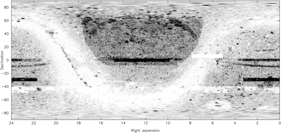
Figure 1: A whole-sky optical density map of all 501,761 objects presented in the QORG catalogue. See the text and the Appendix for details. The pixels at high declinations have been stretched so that a given shade of grey represents the same density of objects per unit solid angle.

5 Summary

This paper presents the QORG All-Sky Optical Catalogue of Radio/X-ray Objects, which is intended to be a grand compilation of the large-scale surveys of the radio and X-ray sky as they existed before the beginning of XMM and Chandra operations. It uses the completed ROSAT, NVSS and FIRST catalogues and the SUMSS catalogue at 70% completion. It provides optical associations for these together with comprehensive identifications of known objects with the intention of presenting an informative map to help formulate and support pointed investigations.

Appendix A Details of the catalogue construction

A.1 The Optical Catalogue used in QORG

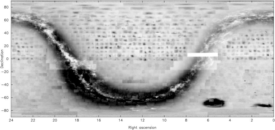
Figure 2: A whole-sky optical density map of the sources in the optical catalogue. The missing sky coverage (white strip at centre-right) is due to corrupt USNO-A data; see the text for details.

The APM and USNO-A catalogues have been combined into a whole-sky 670,925,779-object photometrically recalibrated catalogue. This was done to provide an efficient and uniform optical background against which to perform all other tasks. It was decided at the outset to store astrometric positions to a precision of 1 arcsec only, as early matching across APM plates showed typical discrepancies on the plate margins of up to 2 arcsec from the mean, and we had no desire for precision to exceed accuracy. The USNO-A catalogues have nominal astrometric precision of 0.5 arcsec, but the APM astrometry was selected where available because it is photometrically deeper than USNO-A, and so should be used to ensure the best local astrometric consistency of the merged data. Similarly, it was decided to store photometry to a precision of 0.1 mag only, as early analysis across APM plates showed 20% of matching objects to have photometric scatter greater than 0.3 mag, thus providing a sense of its accuracy. Use of this modest precision standard enables our final optical catalogue to be stored at just 7 bytes per object, converted to 11 bytes per object in our work files, which allows speedy processing for whole-sky tasks. The density of objects on the sky in the resulting catalogue is plotted in Fig. 2.

The APM and USNO-A present their data differently and, in a sense, complement each other. The APM classifies the point-spread function (PSF) of each object as stellar, non-stellar (i.e. galaxy), merged, or non- morphological, and seeks to display galaxy sizes, shapes, and position angles by using ellipses to model isophotally-bounded areas. The downside of this is that close point-sources are often collected by the APM into a ‘merged’ object indistinguishable from a galaxy. The USNO-A is oriented to displaying stars so has no PSF classification and just describes point- positions and magnitudes, but this means no distinction is made between stars and galaxies. By merging these two catalogues together, one gets both kinds of information, and sometimes a bit extra. APM ‘merged’ objects are often resolved by the USNO-A into constituent point sources. Often photometry of different sections of a galaxy becomes available. And where an APM ellipse has a single USNO-A point source positioned at one end of the ellipse with no other USNO-A object present, the properties of an object at the other end can be calculated; comparison with Digitized Sky Survey (DSS) images show that the calculated object is correct to within a few arcsec in position and 1-2 mag photometrically. Such objects have been included in our optical catalogue and are flagged as ‘inferred objects’. Any APM ‘merged’ object that we have resolved into constituent point sources is dropped while the resolved sources are included in our optical catalogue.

Some issues encountered in reading the APM data were:

1. Some APM plates were missing their calibration parameters, so default values were supplied which were later adjusted in the subsequent whole-sky calibration exercise.

2. About 10 of our 1997-dated POSSI-based files were missing J2000 coefficients in the headers. This was remedied by mapping individual objects from the B1950 positions using the transformation matrix from Murray (1989) which was found to yield J2000 positions accurate to within the required arcsec precision.

3. Overly-flattened ellipses were found to be spurious signals. A threshold was established to remove such objects. Also, the APM has a photometric classification for static-like (non-morphological) signals; it was found that objects having only this classification were usually false positives and so were removed. We felt that any true objects thus lost would generally be restored with the subsequent addition of the USNO-A data.

4. Many point sources are seen in only one colour as the counterpart of the other colour is fainter than the plate depth. Sometimes, however, a point source in one colour has its counterpart of the other colour concealed within a ‘merged’ ellipse with an offset centroid, so appearing to be entirely missing in that colour. We felt it important to distinguish between such concealment and genuine absence, so in such cases we have filled out the object data by adding the ellipse photometry for the missing colour.

5. About half of the POSS-I plates contain spurious one-colour ‘objects’ positioned preferentially toward the plate centres; this is evident on the optical density chart of Fig. 2. They are an artefact on the glass copies of the POSS-I plates which originated from defects in the older 103aE and O emulsions that were most strongly imaged in the central area during the copying process. These are very faint but were detected by the deep APM scans of those glass copies (M. Irwin, private communication). In worst cases these can double the nominal population of a POSS-I plate, but they have been found via pattern analysis to have had no discernible effect on our efforts; we have probably benefitted from our approach of matching optical objects to radio/X-ray detections, which also confirms that the matched object is likely to be real. See MWHB section 3.5, where they similarly find that FIRST detections confirm matching APM ‘noise’ objects as likely to be real.

6. Large isophotal ellipses within large galaxies can be astrometrically misaligned between red and blue plates, causing APM to display neighbouring pairs of notional one-colour or mismatched-colour ‘objects’, one blue and the other red, both non-stellar. There was no simple fix for this which would not introduce errors, so such data within large galaxies originate from this artefact.

7. To allow easy reference from a lookup table, we chose to crop each APM plate to the maximal simple rectangle of sky bounded by two longitudes and two latitudes (J2000) - some care was needed in this to avoid loss of sky coverage, i.e. each cropped plate must at least reach all its neighbours. This task was made more delicate by the fact that the original plates were arrayed by B1950 coordinates which are at a small angle to our J2000 boundaries.

8. An APM plate solution designed to correct astrometric plate distortion is available, but we chose to use the raw APM astrometry due to the complex nature of the solution. In this we feel justified by the findings of MWHB that the plate solution actually increases offsets of faint objects near the plate corners. In general our raw APM astrometry is correct to an error of 1 arcsec in RA and DEC, with occasional errors of 2 arcsec in RA and DEC as determined by comparison to FIRST astrometry; see MWHB for a full discussion of these issues.

Some issues encountered in using the USNO-A data were:

1. At the POSS-I and UKST source-plate boundaries (within the USNO-A data) it frequently occurs that an object is represented twice, being on both sides of the boundary. Such duplicate objects within a 4-arcsec separation were removed.

2. Data for 17 northern-sky POSS-I plates were found to be corrupted in both A1.0 and A2.0 catalogues, i.e. basically empty of data there. The affected area is bounded roughly by RA 5h-12h and DEC $3\degr$ – $8.3\degr$. Half of this is covered by the APM, leaving the area bounded by RA 5.6h-8.3h and DEC $3\degr$–$8.3\degr$ (about 243.7 sq deg, 0.59% of the sky) without coverage in our optical catalogue.

3. Similar corruption occurs in 17 southern-sky plates in the A2.0 catalogue. Fortunately the A1.0 catalogue has no problems here, so it was used to populate this region of sky. Oddly, the affected USNO-A plates are those numbered 537 – 553 in each hemisphere.

4. There are substantial photometric zero- point offsets in the A2.0 catalogue; the listed values are nearly a full magnitude too bright, except for red POSS-I $E$ data. The problem was remedied via calibration into APM-governed magnitude ranges. The A1.0 catalogue is not thus affected and seems well calibrated.

5. Southern- sky POSS-I plates displayed a systematic pattern of objects being 0.3 mag fainter at the south end of each plate compared with objects at the north end. This presumably results from the thicker sky cover at lower angles.

Our optical catalogue was initially assembled one APM-based plate at a time by adding in corresponding data from the USNO-A2.0 catalogue, as well as USNO-A1.0 as needed. Objects were matched across input catalogues to a separation of 3 arcsec in each of RA and DEC regardless of photometry, while accommodating best fits for objects multiply packed more closely together. Intra-plate photometric calibration was done separately for red and blue by establishing the median offset between the APM and USNO-A2.0 data, then adjusting the USNO-A2.0 magnitudes by that amount to attain the APM standard; this was done separately for USNO-A1.0 data where we used it. Our optical catalogue retains only a single red and blue magnitude value for each object, so the APM photometry was retained as the first choice in all cases except when the only available POSS-I photometry was from USNO-A, as POSS-I magnitudes are preferred. This is because (a) POSS-I $E$ (red) and $O$ (blue) plates were photographed on the same night, thus ensuring the colour magnitudes are comparable. By contrast, UKST $R$ (red) and $Bj$ (blue) plates are often obtained e.g. 10 years apart, so variability can spoil the colour comparison. (b) POSS-I $O$ is centred on violet, 4050Å, making a broader colour baseline with the red 6400Å (for both POSS-I $E$ and UKST $R$) than does UKST $Bj$ 4850Å. We have found, from 2227162 stellar objects on overlapping equatorial POSS-I / UKST plates after calibration, that the median value of $(Bj-R)/(O-E)$ was 0.65.

After assembly of 824 two-colour APM-based plates (i.e. all those available in 1999, with two overlapping North pole plates treated as a single plate), next came the task of whole-sky photometric calibration. The APM photometry was recalibrated plate by plate by comparing magnitude values of matched objects on cropped plate overlaps, rolled up into a median offset for each two-plate combination. The POSS-I plates were calibrated together in one exercise, the UKST in another. Objects used were those of stellar PSF in both colours on both plates and with positions that agreed to within 2 arcsec inclusive in both RA and DEC - the closer criterion was used to ensure true matches. Calibration was done by adjusting all plate magnitudes by half of the indicated amounts from overlapping areas, then repeating until near-stability was reached, i.e. to where the absolute change per plate averaged less than 1/200th of a magnitude. This took 15 iterations to achieve for the POSS-I plates, and 10 iterations for the UKST plates. The photometric scatter about the median offsets is displayed in Table 1, astrometric scatter in Table 2. The final magnitudes were rounded to 0.1 mag, as described above.

The calibrated magnitudes of objects from APM POSS-I plates were found to vary from the nominal values mostly within a range of $\pm 0.4$ mag, but discrepancies of up to a full magnitude were found. The UKST plates were more stable. The calibrated APM POSS-I $E$ plates were found to have a zero- point offset of 0.2 mag compared with the UKST; that is, the $E$ plates were nominally on average 0.2 mag too bright. After confirmation (Mike Irwin, private communication), all POSS-I $E$ magnitudes were made 0.2 mag fainter. The outcome of the full calibration shows that POSS-I plates are often considerably deeper than the nominal magnitude limit. An extreme example is eo789 which calibrates as having a depth of $E=21.2$ and $O=22.7$, easily deeper than the POSS-II coverage there, confirmed by examining DSS images. Of course, other POSS-I plates can turn out quite shallow, e.g. eo774 with a depth of $E=19.1$ and $O=20.2$. One particularly notable result was that the Large Magellanic Cloud plate f056 was calibrated into being over a full magnitude brighter than APM nominal. The 3823 overlapping stars which yielded this result were carefully examined, and the offset was found to be uniform with normal scatter. The brighter LMC magnitudes are included in our optical catalogue.

134 additional two-colour APM plates were obtained in March 2002, all but one in the southern hemisphere, and these were added by reconstituting the final catalogue in those places using the same processing rules. These new plates were calibrated to the QORG baseline by comparing stellar objects on overlapping plate margins and simply adjusting by the offset median. Our calibration is listed plate-by-plate at http://quasars.org/docs/QORG-APM-USNO-calibration.txt, which also lists the MWHB POSS-I E calibration of 148 of these APM plates using APS. Table 3 summarizes this calibration of all 958 APM-based plates.

It remained to calibrate the large Galactic plane area, which is covered only by the USNO-A. The APM-based plates showed the median adjustments for USNO-A2.0 were to add +0.2 to POSS-I $E$ and +0.8 to POSS-I $O$, and +0.9 to UKST R and +0.7 to UKST $Bj$; see the aggregate summary in Table 3. These offsets were applied to all USNO-A2.0-only areas, except that north of declination $+63\degr$ the local APM-based plates indicated a POSS-I $O$ adjustment of just +0.3; the half-magnitude difference indicates the limit of our ability to bulk calibrate the USNO-A data in the absence of co-positioned APM data. These Galactic plane adjustments completed the photometric recalibration of our optical catalogue.

Preparatory to assembling our all-sky catalogue, we needed to integrate the APM-based equator which is covered by both POSS-I and UKST plates. We combined these by matching objects with positions that agreed to within a separation of 3 arcsec inclusive in each of RA and DEC. The UKST plates are generally deeper than POSS-I plates and so have more objects; thus, we use UKST astrometry where available to preserve local astrometric consistency and provide the most recent position, but we use POSS-I photometry where available, although two-colour UKST objects were chosen over one-colour POSS-I objects. Therefore the result of combining these is an interwoven mix of POSS-I and UKST objects and attributes, with a flag to indicate where the blue magnitude is POSS-I $O$. In this way, 29 equatorial POSS-I plates and 24 UKST plates were entirely written onto their counterparts and so not further used. Similarly, the USNO-A1.0 has POSS-I coverage between $-17\degr$ and $-33\degr$ which is covered in UKST by USNO-A2.0, so the POSS-I data was overlaid onto the UKST background and internally calibrated by adjusting both $E$ and $O$ by the median $(R-E)$ offset for each two-plate combination; this method keeps POSS-I $O$ and UKST $Bj$ photometrically distinct.

The remaining task was to combine all plates into continuous data covering the sky. The recalibrated USNO-A was initially used as the background, to be tiled over by the APM-based plates. Where plates overlap, it is desirable to use the deepest plate; we therefore ordered the plates from lowest plate depth to highest and tiled them onto the background in that order. The deeper plates thus overwrite the shallower ones. Merging was performed at the plate boundaries to ensure no object was lost, as well as de-duplication to a separation of 3 arcsec in each of RA and DEC. Post-assembly analysis revealed some small ‘holes’ in the sky coverage which were manually repopulated from whichever APM plate had the data. As mentioned, the astrometric precision of the final optical catalogue is to one arcsec only. This allocates 1,296,000 R.A. units along the equator. These units naturally compress toward the celestial poles. To ease processing, we allocate only 432,000 R.A. units between declinations $60\degr$ and $75\degr$, 259200 R.A. units between declinations $75\degr$ and $85\degr$, and just 86400 R.A. units poleward of declination $85\degr$. These roundings conform to the 1 arcsec astrometric precision for which we are aiming.

The finished optical catalogue has 155,108,493 POSS-I sources and 112,827,180 UKST sources from the APM, and 192,176,786 POSS-I sources and 210,533,717 UKST sources from USNO-A. These crisp photometric totals mask the fact that many of these QORG optical objects are two-epoch hybrids having POSS-I photometry and UKST astrometry. There are in addition a total of 279,603 inferred objects which appear only in this catalogue, 133,018 inferred from POSS-I data and 146,585 from UKST data. As there is no PSF information on inferred objects we treat them as non-APM except for 286 which are matched in the other colour to an unresolved off-centre APM ‘merged’ ellipse and so are treated as APM-type due to their nominal PSF. All of these add up to 670,925,779 unique objects in the QORG optical catalogue, which maps the sky north of $+3\degr$ in POSS-I, south of $-33\degr$ in UKST, the Galactic plane north of $-17\degr$ in POSS-I, and the remainder in a two-epoch mix of both. A comprehensive listing of individual cropped-plate sky boundaries, plate depths, and counts of the objects categorized by PSF type can be found in the file http://quasars.org/docs/QORG-plate-summary.txt . Table 4 displays the object totals for our optical catalogue where each of our two-colour processed plates is allocated wholly by survey (POSS-I/UKST/BOTH) and source catalogue (APM/USNO-A). These finished processed plates share no objects with their neighbours and can have irregular boundaries and residues of objects from adjacent areas, e.g., the POSS-I plates can contain some UKST objects where they border on UKST areas. These aggregate totals summarize the integrated optical catalogue that we have used throughout this project.

Of particular note in Table 4 are the two-epoch objects. Our optical data retains no explicit two-epoch flag (except where the object is flagged as variable or having proper motion), but since we retain the POSS-I photometry for all such two-epoch matches, and $\sim 98$% of POSS-I objects in this sector have UKST counterparts, we can make the general statement that all objects in this sector annotated as POSS-I are two- epoch in our catalogue, and UKST objects are not, i.e., there was no good POSS-I match for those UKST objects. An exception is the equatorial plates that were covered by APM in both POSS-I and UKST; here we find that about 16% of the flagged 2-epoch objects are in fact UKST from overlapping APM SERC plates. Additional two-epoch objects come from such overlaps of our cropped APM-based plates, for which we evaluated only objects that were stellar in both colours when calibrating our optical catalogue; we retained only those two-epoch objects from the APM overlaps. APM POSS-I plates are $6.5\degr$ on a side and positioned at $6\degr$ intervals, so two-epoch areas are small to begin with; after our cropping and object selection we retained only 1.2% of all objects as two- epoch, as shown in Table 4. The APM UKST plates are also $6.5\degr$ square but are positioned at just $5\degr$ intervals, which optimally allows 70% two-epoch coverage; however, the usefulness of two- epoch UKST coverage is tempered by the UKST red and blue images being taken at different epochs, so that variability and proper motion can be jumbled and lost; after our cropping and object selection we retained only 8.7% of all objects as two-epoch. In total 10.7% of our optical catalogue objects are sourced from two epochs, comprising 18 per cent ($\sim 62200000/347418297$) of POSS-I objects and just 3% ($\sim 10000000/323507482$) of UKST objects; the prevalence of POSS-I two-epoch objects, again, is a consequence of our systematic retention of two-colour POSS-I photometry wherever available.

A token effort was made to detect variability and proper motion across epochs in our data prior to the final assembly of our optical catalogue. Matched objects with post-calibration variability of over 1.0 mag (exclusive) in each colour have been flagged as variable, although where both epochs were APM then the threshold is 0.5 mag because of the uniformity of the calibrated APM photometry. We flag 3,702,933 such objects in our complete two-epoch zone between declinations $+3\degr$ and $-33\degr$, comprising about 5.7% of all objects there. Testing of GCVS stars (for which there is no published completeness) in our two- epoch zone shows we flag 283 out of 851 GCVS stars there as variable for a 33% identification rate, which is a fair result given that many of these stars will have been at equivalent points of their light curves in both epochs, or at different points of their light curves for the discrete epochs of the UKST-R and UKST-Bj plates, which would confuse the comparison to the POSS-I data. In regard to proper motion, matched stellar objects with post-astrometric-calibration positional shifts of 3-8 arcsec have been flagged in our optical catalogue as displaying proper motion; these total 871,705, comprising 1.2% of all our two-epoch objects. We have tested our results against those stars from the Tycho and NLTT surveys which are listed with proper motions of $>0.08$ arcsec/year which should show up as a 3-arcsec shift across the $\sim 30$-year span of our two epochs. We test against Tycho stars in our complete two-epoch zone (as with GCVS) and our optical catalogue flags 6753 out of 15515 qualifying Tycho stars as moving, for a 43.5% identification rate, which seems low; however, these are bright stars, many of which were astometrically inserted into the USNO-A instead of using standard PMM reductions. The NLTT lists faint moving stars perhaps more suited to comparison to our optical catalogue; it has 36,085 stars, being 90% complete over 44% of the sky. Testing against the NLTT over the entire sky shows our optical catalogue flags as moving 3402 out of 33,975 qualifying NLTT stars that we find in our catalogue. As our whole- sky two-epoch completeness is just 10.7% this indicates a $\sim 93$% ($3402/(33975\times.107)$) identification rate of NLTT stars as moving. While at first glance this looks pretty good, further inspection shows that the completeness of NLTT indicates that there should be only about 91,000 such high proper-motion stars over the whole sky, whereas we flag 871,705 such objects, so we have about ten times too many. By comparison, Gould (2003) notes that the USNO-B catalogue (Monet et al. 2003) flags one hundred times too many high proper-motion stars compared with NLTT, but the USNO-B authors elected to over-report as a method of designating high proper motion candidates. Our goal was simply to accurately identify these objects, so it seems that we have overreached somewhat. Our partial success in flagging variable and proper motion objects shows that these flags should be taken as indicative only, and needing confirmation in individual cases.

Table 3: Photometric scatter about the median offset for matched objects on overlapping APM plates. All included objects have stellar PSF in both colours on both plates.

	POSS-I $E$		POSS-I $O$		UKST $R$		UKST $Bj$
Magnitude	Number of	Cumulative	Number of	Cumulative	Number of	Cumulative	Number of	Cumulative
difference	matches	percentage	matches	percentage	matches	percentage	matches	percentage
0.0	256530	16.24	232634	14.73	1317056	24.32	985544	18.20
0.1	446552	44.52	416090	41.07	2039190	61.98	1703200	49.65
0.2	311352	64.23	309549	60.67	1061705	81.58	1149693	70.88
0.3	192744	76.43	204464	73.62	483864	90.52	668240	83.22
0.4	117074	83.85	129618	81.83	228729	94.74	371877	90.09
0.5	72618	88.45	84078	87.15	115546	96.87	206804	93.91
0.6	47723	91.47	56436	90.72	60490	97.99	118176	96.09
0.7	32845	93.55	39041	93.20	33789	98.61	68602	97.35
0.8	22946	95.00	27518	94.94	20956	99.00	41267	98.12
0.9	16581	96.05	19822	96.19	13467	99.25	25972	98.60
1.0	12418	96.84	13829	97.07	9301	99.42	16849	98.91
1.1	9589	97.44	10237	97.72	6590	99.54	11844	99.13
1.2	7298	97.90	7550	98.20	4833	99.63	8866	99.29
1.3	5730	98.27	5679	98.56	3716	99.70	6827	99.42
1.4	4699	98.56	4204	98.82	2781	99.75	5554	99.52
1.5	3754	98.80	3307	99.03	2235	99.79	4383	99.60
1.6	3014	98.99	2717	99.20	1794	99.83	3570	99.67
1.7	2509	99.15	2151	99.34	1436	99.85	3037	99.72
1.8	2083	99.28	1770	99.45	1209	99.88	2532	99.77
1.9	1788	99.40	1410	99.54	1010	99.89	2134	99.81
2.0+	9518	100.00	7261	100.00	5704	100.00	10430	100.00
Total	1579365		1579365		5415401		5415401

Table 4: Astrometric scatter about the median offset for matched stellar objects on overlapping APM plates. All included objects have stellar PSF in both colours on both plates. Note: selection effect at 3 arcsec; multiply number of objects by 3 to obtain true background approx.

Scatter	POSS-I				UKST
(arcsec)	Number in Dec.	Percentage	Number in RA	Percentage	Number in Dec.	Percentage	Number in RA	Percentage
0	848948	53.75	691329	43.77	3376931	62.36	2977660	54.99
1	663282	42.00	785769	49.75	1991025	36.77	2297920	42.43
2	65641	4.16	100762	6.38	47338	0.87	139132	2.57
3	1494	0.09	1505	0.10	107	0.00	689	0.01
Total	1579365	100.00	1579365	100.00	5415401	100.00	5415401	100.00

Table 5: Photometric calibration of the APM and USNO-A2.0 catalogue summarized by plate depth adjustment. The three right-hand columns compare the calibration of 148 POSS-I E plates by MWHB and this paper. Columns are as follows (1) classification: magnitude amount added to plate depth to obtain new plate depth (2) Number of POSS-I $E$ plates, from APM depth to QORG depth (3) Number of POSS-I $O$ plates, from APM depth to QORG depth (4) Number of UKST $R$ plates, from APM depth to QORG depth (5) Number of UKST $Bj$ plates, from APM depth to QORG depth (6) Number of POSS-I $E$ plates, from USNO-A2.0 depth to QORG depth (7) Number of POSS-I $O$ plates, from USNO-A2.0 depth to QORG depth (8) Number of UKST $R$ plates, from USNO-A2.0 depth to QORG depth (9) Number of UKST $Bj$ plates, from USNO-A2.0 depth to QORG depth (10) 148 POSS-I E plates, from APM depth to MWHB depth (rounded to 0.1 mag) (11) The same 148 plates, from APM depth to QORG depth (this is a subset of column 2) (12) The same 148 plates, from MWHB depth to QORG depth.

(1)	(2)	(3)	(4)	(5)	(6)	(7)	(8)	(9)	(10)	(11)	(12)
$-1.4$	.	.	.	1	.	.	.		.	.	.
$-1.2$	.	1	.	.	.	.	.		.	.	.
$-1.1$	.	1	.	.	.	.	.		.	.	.
$-1.0$	1	1	1	2	.	.	.		.	.	.
$-0.9$	1	.	.	.	.	.	.		.	.	.
$-0.8$	.	.	.	.	.	.	.		1	.	.
$-0.7$	1	2	1	4	.	.	.	1	.	.	.
$-0.6$	3	7	.	6	.	.	.		2	1	.
$-0.5$	3	8	6	11	.	.	.		1	1	.
$-0.4$	3	21	15	18	.	.	.		3	.	3
$-0.3$	5	29	36	46	.	.	.		6	.	3
$-0.2$	25	54	60	39	.	.	.		5	5	17
$-0.1$	34	61	89	92	7	.	1		13	10	25
0.0	48	73	123	105	49	.	.		17	19	29
0.1	60	60	91	91	102	.	.	1	11	17	28
0.2	74	57	45	43	90	4	.		23	27	24
0.3	68	47	22	25	84	2	.	4	20	21	11
0.4	50	16	10	13	57	4	7	15	19	16	4
0.5	40	4	7	5	34	26	3	26	14	20	1
0.6	19	4	2	7	12	59	22	63	8	7	3
0.7	6	.	1	1	2	110	42	71	3	2	.
0.8	4	1	1	1	1	90	46	53	1	2	.
0.9	2	1	.	.	.	62	65	37	1	.	.
1.0	.	.	.	.	.	39	42	16	.	.	.
1.1	.	.	.	.	.	22	25	7	.	.	.
1.2	1	.	.	.	.	15	23	7	.	.	.
1.3	.	.	.	.	.	2	13	5	.	.	.
1.4	.	.	.	.	.	2	11		.	.	.
1.5	.	.	.	.	.	1	4		.	.	.
1.6	.	.	.	.	.	.	1		.	.	.
1.7	.	.	.	.	.	.	1		.	.	.
Total	448	448	510	510	438	438	306	306	148	148	148

Table 6: Counts of optical objects in the QORG optical catalogue, subdivided by POSS-I/UKST surveyed areas (‘BOTH’ indicates 2-epoch areas) and source APM/USNO-A catalogue. Note that all 2-epoch objects from areas surveyed by both POSS-I and UKST are POSS-I, as POSS-I photometry was always retained for these.

	Source	No. of $R$+$B$	Area	No. of optical	No. of POSS-I	No. of UKST	No. of 2-epoch	2-epoch
Survey	Catalogue	plates	(sq deg)	objects	objects	objects	objects	percentage
POSSI	APM & USNO-A	448	13504.9	133053261	133046581	6680	1579365	1.2
POSSI	USNO-A only	296	5799.1	149390371	149204938	185433	0	0
UKST	APM & USNO-A	201	4534.7	62582083	20972	62561111	5415401	8.7
UKST	USNO-A only	207	4857.8	170296427	45907	170250520	0	0
BOTH	APM & USNO-A	309	7977.7	82968412	27932578	55035834	$\sim 28000000$	33.7
BOTH	USNO-A only	76	4335.0	72635225	37167321	35467904	$\sim 37000000$	51.0
TOTAL		1537	41009.3	670925779	347418297	323507482	$\sim 72000000$	10.7

A.2 Calculation of the Likelihood of Association between Optical Objects and Radio / X-ray Sources

The distinguishing technique of the QORG catalogue is the uniform algorithm by which likelihood of association between optical and radio/X- ray sources is calculated. The naïve approach to causal linking of these would be to search for simple astrometric co-positionality, but problems with that approach include the natural offsets in extended objects and jets and lobes, the astrometric imprecision of the available data, especially the X-ray data, and the differing significance of co- positionality in dense star fields compared to sparse. The FIRST Bright Quasar Survey (FBQS: White et al. 2000) aligned radio and optical astrometry to a precision of 0.1 arcsec and found that co-positionality was a sufficient sole criterion for association only out to a 1.2 arcsec separation in sky areas away from the Galactic plane. The present work treats positional separation only in increments of 1 arcsec, and uses this with additional criteria to quantify likelihood of association. As an example, given two equivalent nearby optical candidates for association with a radio/X-ray source, if one of them has R = B and the other has R = B - 2.5, we would consider the former to be the far more likely candidate as it has QSO-like colours, while the other is likely to be a coincident star. But to weigh this distinction accurately requires quantitative assessment of the likelihoods to be assigned to different optical colour bins. In total we use three observational parameters to assess the likelihood of association between radio/X-ray sources and optical candidates: astrometric offset, B - R colour, and APM PSF classification in each colour.

Likelihood is gauged by comparative density on the sky. If, say, stellar- PSF objects of R = B on annuli 5 arcsec from the set of all RASS X-ray sources are 10 times as dense on the sky there compared with the all-sky (background) density, then we say the chance of association of those optical objects there is 90%, i.e. of each 10 of those optical objects, we take one as typical background and the excess 9 as causal. This approach must incorporate local sky object density, as otherwise calculated likelihoods in densely-populated areas would be falsely high against the all-sky-average background. A simple local density-dependent multiplier would suffice in one sense, but this would overlook the different mix of objects in different parts of the sky, i.e. the low- density Galactic caps are expected to have a higher ratio of objects with QSO-like colours than the high-density Galactic plane. To accommodate both density and object-mix variations, we have divided the sky into twelve sky density bins, and accordingly have broken our optical catalogue out into rectangles of approx 1 sq degree and allocated them by mean object density into those twelve bins. Table 5 shows the areas, object counts, and average densities for the total objects and the APM-only objects, for each sky density bin. These density bins have been designed to keep the discrepancy between any local sky density and the density of the corresponding bin to a maximum of 20%, although greater discrepancies are possible in inhomogeneous areas, of course. A 20 per cent density error will result in a likelihood figure of e.g., 90 per cent, to be written as 88% or 92%(see equation 2, below), which we consider acceptable.

Table 7: 12 sky density bins and summations of the sky portion allocated to each bin. Note that 243.71 square degrees are missing from the optical catalogue.

Density	Density range	Total area	Total no.	Mean	APM Area	APM no.	APM mean
bin	(per square degree)	(square degree)	objects	density	(square degree)	objects	density
6000	1– 6000	3206.24	15533000	4845	2757.65	13057871	4735
8000	6001–8000	5416.09	38352783	7081	4815.15	33185681	6892
10000	8001–10000	7333.54	65955475	8994	6382.29	56028957	8779
12000	10001–12000	6018.01	65589155	10899	4916.19	52348586	10648
15000	12001–15000	5591.52	74376431	13302	4039.37	52316607	12952
18000	15001–18000	3299.59	53680671	16269	1801.29	28611437	15884
22000	18001–22000	2409.98	46968715	19489	796.56	15306870	19216
34000	22001–34000	3539.80	94724199	26760	405.07	10157923	25077
45000	34001–45000	2380.68	93561653	39300	31.81	1197891	37657
60000	45001–60000	1144.29	56432307	49317	23.21	1223691	52712
100000	60001–100000	347.90	27239742	78298	32.18	2529866	78608
150000	over 100000	321.63	38511648	119740	16.54	1970579	119123
Total		41009.25	670925779	16360	26017.32	267935959	10298

These binned areas and counts of objects serve as background denominators for our likelihood calculations. For objects with APM PSF information we use the APM areas and counts, for non-APM we use the total areas and counts. One remaining division in our sky is that of POSS-I versus UKST objects. As previously stated, UKST ($Bj-R$) is 0.65 of POSS-I ($O-E$) as a median, so an object typically will have a larger colour spread in POSS-I than in UKST. Early pre-publication versions of our catalogue calculated denominators separately for each survey, thus doubling the number of bins and so reducing their population. However, it is desirable to keep our background bin populations as large as possible to minimize statistical fluctuations. We judge that it is qualitatively preferable to use a simple statistical rule to align the UKST colours to the POSS-I colours, thus keeping these objects unified within the same bins. Thus we chose to multiply each UKST object’s $(Bj-R)$ by 1.5 ($\sim 1/0.65$) to map to the statistically expected POSS-I $(O-E)$, for $Bj>R$. The result is that the 12 sky density bins of Table 5 represent the starting pools of data for all likelihood calculations. During each such calculation, the appropriate pool was divided up by APM PSF class and O-E colour to obtain the required background denominator.

Our APM-style PSF classification takes on just 4 discrete values for each colour: stellar (written by us as ‘-’ as a truncation of APM’s ‘-1’), fuzzy (‘1’), extended (‘2’) and no classification (‘n’). Our stellar and fuzzy classes come straight from the APM, but our extended class ‘2’ differs from the APM merged-object ‘2’ in that we expect that such a source should have a visible source at the centroid, or be a component of a large galaxy. If the PSF is not classified as ‘-’, ‘1’, or ‘2’, then we take it as an ‘n’ for these likelihood calculations even if the colour is missing, as the question here is not the visibility but just the morphology. All objects are also accumulated into the PSF-free ‘n’ class in each colour (without double-counting if it is already ‘n’), and again with ‘n’ for both colours. Thus, with just four PSF classifications available for each of two colours, we have a total of 16 two-colour PSF bins.

O-E colour is binned by 0.3 to keep bin populations large while blurring colours by no more than 0.1 mag. We use the range ($-0.9\leq O-E\leq 4.5$), binned by 0.3, with $O-E<-0.9$ taken as -0.9 and $O-E>4.5$ taken as 4.5. As mentioned, for UKST $Bj>R$, we take $O-E=(Bj-R)\times 1.5$, then bin it in the same way. One-colour objects have no $O-E$, but are included in a cumulation of all objects which is given a placeholder value of $O-E=9.9$. Thus we have a total of 20 $O-E$ colour bins. Note that there is an APM photometry artefact in dense LMC areas which results in an overabundance of $Bj\ll R$ in the two highest density APM bins; possibly the APM confused near neighbours when matching images across colours. The consequence is that we cannot use the colour criterion in the LMC. Without this tool, and in recognition that our methods are less effective in very dense star fields, to deter false positives we have chosen to require co-positional fit within 1 arcsec to accept association in the two highest density bins of 100000 and 150000.

The breakdown of our optical catalogue into these cross-categories of 12 sky density bins by 16 PSF bins by 20 colour bins is displayed at http://quasars.org/docs/QORG-background.txt . The total number and APM number of objects for each of the 3840 cross-indexed bins are listed. For each likelihood calculation, a cross-indexed bin is selected using the optical object’s attributes, and that bin provides the background numbers used for the denominator.

Likelihood is calculated in terms of the overabundance of optical objects over the background. As an example calculation, let us consider a HRI source offset 3 arcsec from an optical object which is stellar in both colours, has $O-E=0.3$, and is located in sky of density bin 8000. Our input HRI catalogue has 6859 X-ray sources in sky of density bin 8000; therefore for offset annuli of 3 arcsec about these, the total area (between radii 2.5 and 3.5 arcsec) is 129,289 arcsec², and within this area of sky our optical catalogue yields 31 objects (smoothed) which are stellar in both colours and $O-E=0.3$. Table 5 shows that the all-sky area of density bin 8000 is 4815.15 sq deg which converts to 62,404,324,852 arcsec², and within this sky area the background count of objects which are stellar in both colours and $O-E=0.3$ is 213,453, as shown in ‘QORG-background.txt’. The comparative sky density for these optical objects at 3 arcsec offset from HRI sources is thus

$${\rm Density} = ({\rm count}/{\rm area})/({\rm background\ count}/{\rm background\ area})$$ (1)

$$= (31/129289{\ \rm arcsec}^{2})/(213453/62404324852{\ \rm arcsec}^{2})$$ (2)

$$= 70.1$$ (3)

The density of 70.1 represents an overdensity of 69.1 compared to the background of 1. Thus confidence of association = $(70.1-1)/70.1=98.6$% for each object, and this is our measure of causal likelihood:

$${\rm Confidence}={({\rm density}-1)\over{\rm density}}$$ (4)

Complete densities and supporting figures are given for all cross-indexed bins for the HRI input catalogue in the density chart at http://quasars.org/docs/QORG-HRI-densities.zip, and similarly for the RASS, PSPC, WGA, NVSS, FIRST and SUMSS input catalogues. Smoothing rules used are itemized in the headers of those files. Note that outlying bins such as that of $O-E=-0.9$ can have very small populations, so to avoid small- numbers fluctuations we have amalgamated the outliers to where the bin population ‘count’ in equation (1) is expected to be at least five. Thus in ‘QORG-HRI-densities.txt’ the first displayed $O-E$ bin is $O-E=0.3$, which includes smaller $O-E$. The need to keep bin populations high shows that the efficacy of our likelihood method is directly dependent on the size of the input catalogue, and indeed small-number fluctuations in outlying bins are an occasional hazard. In the closing section of this paper we describe an offset-dependent penalty which we have deployed to further control this intermittent problem.

There are, however, complications that we needed to resolve before these final densities were written. In the case of the X-ray catalogues, the ROSAT fields are misaligned with respect to the optical background, typically by 1-10 arcsec, and need to be shifted to their correct locations. Some shifting is also needed for the radio fields, but in this case it is because the APM astrometry can be offset from the true by up to 2 arcsec in each of RA and DEC (at the plate edges; see MWHB for a full discussion), and as we use the APM for our reference astrometry we need to realign the radio survey astrometry where appropriate; that is, introduce equal errors so as to align it to our APM background. This is an iterative process as a density chart must be compiled first out of the original astrometry for each radio/X-ray catalogue, then that density chart is used to re-align the astrometry, then a new density chart is compiled using the revised astrometry as an input catalogue, etc. Our experience is that three iterations are sufficient as the fourth brings little change to the density chart. The final density charts are much more focused than the initial ones, with high densities for near positional fits, and densities falling off rapidly outwards, much like the final chart displayed on http://quasars.org/docs/QORG-HRI-densities.zip for HRI; similar results are obtained for the other catalogues. We describe our method for achieving these shifts in the following sections.

A.3 The X-ray Sources

The immediate consideration in using ROSAT X-ray catalogue data is in deciding which source detections to use at all, as their reliability varies and flags are present to signal reduction difficulties due to close or complex sources. Most HRI and PSPC sources bear some of these flags; of the 131,902 total HRI sources, only 13,452 are entirely unflagged. These flags originate from the surveyors’ manual inspection of all the individual detections, and one of the flags signals their overall assessment that the source is a false detection; where this flag is not set, the source was not determined to be spurious. We therefore use onwards all sources without this flag as candidates for matching to our optical catalogue. Of the 131,902 HRI sources, 111,865 are without the false-detection flag; however, of these, 8767 are astrometric duplicates (to the 1-arcsec resolution of this project) within the same ROSAT observing field, and 46,700 further sources are flagged by HRI as ‘non-unique’ astrometric duplicates across different ROSAT fields – this is not unexpected, as many objects of interest were observed repeatedly. Thus in the end we are left with 56,398 astrometrically unique HRI sources to attempt to match to optical objects. Similarly, 100,205 individual PSPC sources are available to us from the 118,785 original sources in the combined PSPC and PSPCF catalogues; these catalogues have no ‘non-unique’ flag. The WGA catalogue authors used a single ‘quality flag’ to gauge reliability, and using their 88,621-record catalogue of ‘good’ sources yields 88,378 individual sources. The RASS catalogue has clean data with only a few complex-emission sources which we have chosen to retain, so we use their full complement of 124,730 sources.

The primary task in associating ROSAT sources with optical objects is that of astrometrically fitting the ROSAT observing fields to the optical background. As detailed in Appendices B and D of the ROSAT User’s Handbook, there were ongoing boresighting and undiagnosed errors which caused pointing unreliability of up to 20 arcsec. This ‘attitude solution error’ was accompanied by a systematic roll angle error of 6 arcsec which has been corrected for in the final HRI, PSPC and RASS catalogues that we use, but the attitude error was more random than systematic and persisted throughout ROSAT’s operation. HRI fields are nominally more precisely pointed than PSPC or RASS, but we find in our analysis (below) that some HRI fields, too, are offset by as much as 15 arcsec; see also Mason et al (2000), figure 1, which shows PSPC sources offset from their optical counterparts by up to 15 arcsec with one source offset by 30 arcsec. WGA fields often have offsets 10 arcsec greater than their corresponding PSPC fields, possibly because of the absence of the roll angle fix combined with an early pointing solution. The question of correctly repointing a ROSAT observing field is present in every instance of its use. Researchers have often resisted shifting the fields lest their analysis be disputed. Our task here, however, explicitly involves causal linking of optical and X-ray sources, and correctly repointing the ROSAT fields is essential to optimizing this task. We believe our likelihood algorithms based on our whole-sky optical data gives us an unprecedented opportunity to decide the correct alignment of the ROSAT fields in bulk.

The general principle of our approach is to find compelling X-ray-optical associations and shift each ROSAT field so as to superpose its X-ray sources perfectly onto the optical background. Of course, the real data never fits perfectly, many X-ray sources have optical counterparts too faint for our optical catalogue, and we need to find quantifications which yield optimal alignments without falling prey to chance coincidental fits. Our main tool is of course the likelihood confidence method explained in the previous section, and we needed to determine the likelihood score for each X-ray-optical association and sum the scores for each ROSAT field in a way which incorporates both (1) the number of associations and (2) the power of precise fitting associations in a balanced way – neither of these is sufficient on its own, as random alignments can easily give rise to many associations at large offsets, or a few small-offset associations. Monte Carlo simulations cannot easily be designed to optimise the combination of these two measures, as we have no a priori notions of what comparative configurations of control and test data should be expected to fit validly, and which would fit only coincidentally. Any simulation- derived rules would need to be tested against real-sky data to find if the simulation was designed in conformance to real-sky behaviour; the requirement for real-sky testing renders the simulation superfluous. Our general approach of being guided by the real data itself to find the rules and numbers applied as strongly here as anywhere else. Thus, in practice, to determine the optimal combination of the above two measures, we heuristically tried different formulations and tested them against well- understood X-ray fields to find the best-performing solution.

We processed each input catalogue (e.g., HRI) separately. Our first step was to compile an initial density chart (as defined in the preceding section) for a whole input catalogue using its nominal (original) ROSAT astrometry. Next we test, for each ROSAT field, all positional shifts from the nominal location out to $\pm 48$ arcsec offset in each of RA and DEC (in intervals of 3 arcsec to save processing, thus 1089 shifts in total). Each tested field shift is scored as follows: first, we use the density chart to produce confidence of association figures for the field’s X-ray- optical matches, using sources singly only; these need to be amalgamated into a final score for that field shift. This final score must incorporate both the number of X-ray-optical matches and their individual confidence scores; thus a summation of confidence scores is indicated, but in testing this against selected fields (notably the quasar-rich environs of NGC 3628) we found that field shifts with many low-confidence matches tended to outscore field shifts with a few high-confidence matches which were in fact correct, judged by co-positionality of X-ray sources to known quasars. We found this problem to be remedied by using the squares of the confidence scores instead of the confidence scores directly; in this way a single 100% match is worth four 50% matches instead of just two. This yielded the correct final astrometry in our test fields. It did not, however, work to use the cubes (etc) of the confidence scores, as then a single randomly-generated precise co-positionality could overpower a small number of valid causal matches. Thus in our summations we define the ‘weight’ of an individual X-ray-optical match to be the square of its confidence figure. We double a weight figure if its optical object is a known QSO, and decrease it up to 33% where the optical astrometry is compromised due to non-stellar morphology or missing $R$ or $B$; again, these corrections evolved heuristically via extensive testing. Only individual weight figures of $>0.5$, corresponding to confidences of $>70$%, are retained to limit the contributions of random matches, and at least two separate X-ray-optical associations must be present for a field shift to be plausibly informative; to shift a field based on a single association prejudges the process. The total weight (score) of the field shift is the sum of the weights of all its individual X-ray-optical combinations.

Of course, the significance of this score depends on the number of X-ray sources in the ROSAT field, which we term $N$. Finding two precise X-ray- optical alignments in a ROSAT field having only two X-ray sources might constitute a compelling field shift, but if the field has 100 X-ray sources, and we have matched only two, then that would be unconvincing. We need to make this quantitative. One might start by considering the contribution of the field’s angular size and photometric depth to $N$, but various studies (including Mason et al. 2000) have found that the associability of X-ray signatures with visible optical sources does not vary much with X-ray flux. Thus we can quantify $N$ directly as the sole counterbalance to our total weight of the field shift; it is the sole counterbalance because on the optical side our density calculations already incorporate the optical object density. We incorporate this quantification $f(N)$ to define the ‘power’ $P$ of the field shift:

$$P=\Sigma({\rm weight})\times f(N)$$

We will find a threshold power value below which we deem that the field shift is not proven and so not used. We find a suitable $f(N)$ by heuristic testing. $f(N)=1/N$ fails because it models match numbers to be increasing linearly with X-ray source numbers, ignoring high match rates randomly obtained in low-density fields, i.e. small-numbers fluctuations; we find that twice the matches in a field with twice the X-ray detections is indeed more significant as our testing shows such field-shifts point more reliably to known quasars. $f(N)=1/{\sqrt{N}}$ is found to model adequately the performance of field shifts using fields of different $N$; this is again a heuristically-gained measure. Thus we define the power of the X-ray- optical alignment of the field as:

$$P=\Sigma({\rm weight})/\sqrt{N}$$ (5)

where $N$ is the number of X-ray sources in the ROSAT field. Note that we thus ascribe the same power to two precise superpositions in a field of four X-ray sources as to 10 precise superpositions in a field of 100 X-ray sources, where other X-ray sources are unmatched to optical. This conforms to our naïve expectation. Large fields with many X-ray sources, such as some RASS fields, will have high power scores only if they are well aligned with the optical background.

However, yet another factor is needed to counteract high weight scores generated randomly at large field shifts; after all, two configurations of random point sources will align optimally, but meaninglessly, somewhere, most likely at large field shifts as the number of candidate field shifts increases linearly with shift distance. Thus, we need an accompanying linearly-dependent penalty to suppress the random outliers. The question basically is that of quantifying the significance of the original astrometry as specified in the ROSAT catalogues. We analyse this by compiling the mean power score of all ROSAT fields over all 1089 candidate shifts, for each ROSAT catalogue, in Table 6. Inspection shows the mean power rating is highest at the original astrometry and falls off with increasing field shift until at high shifts it stabilizes into a background level. The HRI mean power at the original astrometry is less than that of the PSPC because its smaller field sizes provide fewer associations per field. The rapid dropoff of the HRI mean power with increasing field shift shows that it is the best-pointed of the four surveys, and its reaching near-stability at a shift of 21 arcsec indicates that there are no valid HRI field shifts greater than 20 arcsec. The PSPC and WGA powers decline significantly out to about 30 arcsec. The WGA mean power at the original astrometry is small because of its lesser pointing accuracy; in addition, about 30% of the listed WGA fields are amalgamations of multiple PSPC fields for which our field shifting technique is necessarily problematic. The RASS powers in Table 6 are medians as we process RASS differently to the others; we describe this in more detail below.

Table 8: Mean power and total number of $>70$% confidence associations for all ROSAT fields for each catalogue, for candidate shift increments of 3 arcsec. Object numbers increase at higher shifts because of the greater quantity of candidate field shifts. RASS powers are medians.

Field shift	HRI		PSPC		WGA		RASS
(arcsec)	Power	No. objects	Power	No. objects	Power	No. objects	Power	No. objects
0	1.38	2251	1.61	3220	1.07	1792	0.93	1144
3	1.22	16048	1.52	25010	1.05	13960	0.89	9082
6	0.96	19406	1.37	35830	1.02	19944	0.79	13537
9	0.73	19750	1.20	44874	0.98	24940	0.67	17864
12	0.58	29180	1.01	81977	0.92	45276	0.54	35319
15	0.51	20527	0.83	64890	0.84	35261	0.43	30367
18	0.49	26240	0.72	83211	0.76	44561	0.36	42535
21	0.48	24849	0.63	75432	0.69	39375	0.31	41769
24	0.48	29044	0.59	83235	0.62	41781	0.27	49226
27	0.47	40676	0.56	109828	0.57	52335	0.25	68633
30	0.47	33109	0.54	86150	0.53	38722	0.23	55324
33	0.47	42010	0.53	106248	0.52	45635	0.22	69625
36	0.47	39520	0.52	97874	0.50	40444	0.21	64784
39	0.47	50532	0.51	123597	0.50	49278	0.20	82234
42	0.47	50237	0.51	120733	0.50	46913	0.19	80655
45	0.47	46927	0.50	113371	0.49	42863	0.19	75379
48	0.47	61338	0.49	146744	0.49	53524	0.18	97355

We used the power values in Table 6 as our measure of the significance of the nominal astrometry of the four ROSAT catalogues, to be added to the power score of each field shift, thus favouring lesser shifts where all else is equal. Before we added this in, though, we analysed the full set of 1089 candidate shifts for each field to find local power maxima; i.e., field shifts having power values higher than all their neighbouring shifts have, which generally signifies close individual alignments across the X-ray and optical fields. We might find, say, 38 of these, and we use from then on only those 38, which thus avoids skewing positions when adding the values from Table 6. We then added the extra power score from Table 6 according to the field shift in arcsec for each candidate shift, but also subtract the score obtained for no offset zero (e.g. 1.38 for HRI) to normalize the score compared to non-shifting fields; the final effect is that of a penalty against the original astrometry, i.e. the further the candidate shift, the greater the penalty deducted from that candidate’s power score. After applying this penalty, the field shift with the highest total power score exceeding the threshold value of 0.5 is the ‘winning’ field shift, and is used from then on, provided it leads the runner-up power score by at least 0.1 or if both shifts are astrometrically similar – we prefer to use no shift if the top shift candidates are scoring about the same, as can happen especially in dense star fields where random fits often have equally ‘good’ power scores. The 0.5 ($\geq 0.45$) power threshold was found by trial and error and physically corresponds to two 70% confidence associations in a field of four X-ray sources; ‘best’ fields scoring less than this usually look like random fits. The 0.1 power distinction approximately corresponds to the presence of an additional 70% confidence association. As the winning field shift was selected from candidates at intervals of 3 arcsec, we tested further field shifts offset 1 arcsec from the winner to find the one producing the best score; this is the final field shift used. A complete list of the HRI fields and the field shifts used is displayed in http://quasars.org/docs/HRI-fields.txt, and similarly for the RASS, PSPC and WGA input catalogues.

We have established maximum shift values of 18 arcsec for HRI and PSPC and 31 arcsec for WGA. These were not arbitrary decisions but were made after an initial full build without using these maxima, and without using the astrometric significance penalties from Table 6. See http://quasars.org/docs/HRI-shifts-old.ps for the distribution of HRI field shift distances versus power; each field is represented once, by the shift of that field that yields the best power score; similar charts are available for RASS, PSPC and WGA. The graph shows a population along the vertical power axis consisting of high-power ($>1.5$) low-distance ($<10$ arcsec) shifts, and another population along the horizontal shift distance axis consisting of high-distance ($>15$ arcsec) shifts of low power ($<1.5$); these are the randomly-generated field shifts which have no physical significance and arise only because of the sheer volume of high-distance candidate field shifts. We originally tried to draw a dividing line of significance where these two populations meet, which is of course not a clean boundary as valid and invalid shifts are found on either side. Spot checks of all fields in the central vicinity where the dividing line lay revealed that beyond a certain maximum field shift no shift looked compellingly good; either fuzzy or one-colour objects dominated or there were a lack of close positional fits. For HRI we found the maximum good field shift was 18 arcsec and for PSPC we found the same; although we felt PSPC should have some larger good field shifts, given the intrinsically lower resolution of the observations, we could find no compelling instance in our extensive spot checks. The valid-looking shifts all had good power scores, and shifts of similar magnitudes with low power scores looked less compelling on inspection. These low-power shifts are generally removed by the astrometric significance penalty from Table 6. WGA had plausible alignments out to a 31 arcsec shift, and a broad view of http://quasars.org/docs/WGA-shifts.ps shows that as a whole the WGA fields are more free-ranging than HRI or PSPC. Having established these maximal field shift values for HRI, PSPC and WGA, the final full build was done which disallowed consideration of any fields shifts beyond the maxima, and which required any candidate field shift to have a power score $\geq 0.45$ above the astrometric significance penalty from Table 6, as described above. The result for HRI is shown on http://quasars.org/docs/HRI-shifts.ps and similarly for the PSPC and WGA input catalogues.

The RASS differs from the other ROSAT surveys in that its fields are large ($\sim 27$ deg² each) and the exposures comparatively short, with concomitant large uncertainties in the published source positions. We have also encountered astrometric inconsistencies within RASS fields which are possibly due to distortion in the outer off-axis parts of the ROSAT images. Given this graininess of the RASS positions, we have elected to optimize our optical selections by using the HRI and PSPC surveys to ‘anchor’ the RASS fields wherever possible, by correlating high-flux X-ray sources across the three catalogues and designating the corresponding HRI/PSPC-chosen optical objects as highly-weighted targets for the RASS fields. RASS fields without HRI/PSPC overlaps must still rely on astrometric significance penalties to avoid randomly-large shifts, and we find that median-based power values accord best with the grainy RASS astrometry to allow valid-looking large shifts to be selected. A ‘valid- looking large shift’ is one for which associated optical objects have similar PSFs and colours as those associated in fields with small shifts, and which contains some close X-ray-optical positional fits. We found that some large RASS field offsets did fulfil these criteria, so we did not impose a maximum shift value as was done with HRI and PSPC. However, even without such a limit there turn out to be few large RASS field shifts, as seen on http://quasars.org/docs/RASS-shifts.ps . We have checked all fields with shifts of $>14$ arcsec: fields 33023034 at 42 arcsec and 33016040 at 34 arcsec are the two largest shifted fields, and both have multiple good optical fits and sources confirmed by PSPC. All the other fields also look valid except for three low-power fields which looked like random ‘best’ fits: 33025019 at 15 arcsec and 0.7 power, 33012017 at 15 arcsec and 0.9 power and 33031016 at 26 arcsec and 1.1 power. We have manually reset these to zero shift and none contributes any associations to the final catalogue. Having culled these, we are satisfied with the performance of the large RASS field shifts.

Table 7 summarizes all field shifts for the four input ROSAT catalogues, showing the resultant increase in the number of $>70$% confidence X- ray-optical associations. For HRI the number of associations presented in QORG is less than the number of $>70$% confidence associations used to shift the fields; this is because of overlapping-field duplicates which we remove; WGA has few such duplicates, and RASS none. The shift=0 row represent fields which were ‘shifted’ to their original locations; the lack of astrometric penalty at zero shift allows a few low-quality fields to reside there. Unshiftable fields are included for completeness as ‘unshifted’. The high number of WGA fields without a preferred shift is a consequence of their $\sim 1000$ merged fields which cause problems for our analysis, and many HRI fields are left unshifted because they contain few sources; 3288 HRI fields have fewer than 10 sources, compared to 2005 for PSPC.

In all, for shifted fields, HRI shows the high-confidence ($\sim 88$%) X-ray-optical associations expected from their well-pointed high-resolution observations, PSPC’s pointing looks as good but its detections are not as well resolved so positional fluctuations lower the median confidence of X-ray-optical associations to about 79 per cent, WGA’s resolution is the same as PSPC’s but has pointing problems which lower the median confidence of X-ray-optical association to about 70%, and RASS’s pointing is similar to PSPC’s but its resolution appears to be quite grainy with X-ray-optical offsets often in excess of the stated positional uncertainty, which keeps the median confidence of X-ray-optical associations down to about 69%. Table 8 displays the median offset between the original published X-ray position and any optical object which we find to be associated with $>40$% confidence (which is the threshold required for inclusion in QORG), categorized by published positional uncertainty of the X-ray detection; ROSAT duplicate entries are included, and we use the original astrometry to exclude the effect of our field shifting. No RASS sources are published with less than 6 arcsec positional uncertainty. It can be seen that HRI has marginally better accuracy than PSPC, which is in turn marginally better pointed than RASS, which shows the RASS positions to have greater scatter and thus a lower resolution. There is no WGA entry in Table 8 as WGA provides no published positional uncertainty for their detections; their published comment is that the uncertainty is ‘close to 10 arcsec’ which accords well with our finding that the median WGA X-ray-optical offset is 8 arcsec regardless of source flux.

Table 9: Alignment of ROSAT fields: The number of fields shifted as a function of shift distance, with X-ray source numbers, $>70$ per cent-confidence associations used in shifting (both before and after the shift), resultant associations appearing in our catalogue, and the median confidence of those associations. Unshifted fields are included; the absence of a shift is generally due to a lack of good X-ray-optical fits.

	HRI						PSPC
Shift	No.	Orig.	$>70$%	QORG	No. in	Median	No.	Orig	$>70$%	QORG	No. in	Median
(arcsec)	fields	sources	conf	$>70$%conf	QORG	conf.	fields	sources	conf	$>70$% conf	QORG	conf
0	58	961	324	324	270	80	90	2577	948	948	839	77
1	301	3945	1608	1692	1276	88	285	7576	2679	2779	2824	78
2	354	4334	1800	2122	1646	89	324	8920	3008	3412	3231	78
3	480	7331	2345	3022	2549	88	575	14355	4628	5481	5093	78
4	456	6090	1889	2708	2240	88	558	13650	4186	5206	4980	78
5	271	3515	993	1557	1301	88	316	7915	2491	3160	2903	79
6	131	1427	381	712	530	87	274	6177	1767	2386	2311	78
7	92	1075	247	468	417	84	221	4981	1400	2020	1887	78
8	27	209	53	113	85	89	108	2232	581	884	802	78
9	20	182	45	87	72	89	103	1929	517	851	664	79
10	3	33	6	15	15	81	46	808	203	357	276	77
11	4	20	3	16	8	81	27	460	115	207	177	82
12	1	6	1	4	5	84	13	172	39	84	75	82
13	.	.	.	.	.	.	13	248	42	99	59	74
14	1	11	1	8	9	92	7	288	46	99	82	82
15	.	.	.	.	.	.	7	154	32	60	66	79
16	.	.	.	.	.	.	3	37	6	20	18	81
17	1	33	6	13	12	79	1	16	3	8	8	89
18	1	10	.	6	4	88	1	8	1	3	3	87
unshifted	2920	27121	1251	1251	2294	60	2321	29073	1651	1651	3174	58
Total	5121	56303	10953	14118	12733	84	5293	101576	24343	29715	29472	76
	WGA						RASS
Shift	No.	Orig.	$>70$%	QORG	No. in	Median	No.	Orig	$>70$%	QORG	No. in	Median
(arcsec)	fields	sources	conf	$>70$%conf	QORG	conf.	fields	sources	conf	$>70$% conf	QORG	conf
0	14	520	92	92	149	66	41	3672	665	665	1022	71
1	41	1187	264	270	342	70	71	6372	1213	1247	1876	70
2	63	1862	352	405	574	68	88	9683	1711	1863	2935	69
3	114	3872	707	818	1099	67	183	18954	2886	3213	4976	68
4	150	4531	823	991	1284	68	187	19905	2961	3383	5417	67
5	100	2733	501	655	823	70	87	8081	1440	1694	2522	71
6	124	3276	622	813	1033	71	107	9156	1606	1925	2862	69
7	152	4553	814	1103	1438	70	102	9134	1415	1687	2629	69
8	97	2714	482	682	796	72	41	3523	568	725	1044	69
9	131	3636	553	874	1109	71	54	4539	759	962	1461	70
10	94	2779	418	639	824	70	29	2459	334	441	665	67
11	88	2493	377	620	761	69	18	1461	209	290	413	69
12	78	2485	319	617	731	71	11	764	86	121	183	68
13	40	1112	134	279	335	71	10	727	117	158	226	67
14	50	1304	167	351	462	71	2	149	14	28	43	71
15	45	1420	182	346	463	70	4	413	49	51	70	68
16	32	729	92	207	225	74	2	152	18	21	36	75
17	16	452	57	124	128	73	.	.		.	.	.
18	11	225	21	62	70	79	.	.		.	.	.
19	13	317	40	99	98	77	3	167	4	14	36	58
20	9	233	30	73	61	75	1	90	3	6	15	49
21	7	130	19	54	29	69	2	80	4	8	11	63
22	8	236	17	62	87	73	.	.		.	.	.
23	6	74	11	27	20	77	.	.		.	.	.
24	5	134	11	38	49	70	.	.		.	.	.
25+	18	324	33	103	66	72	2	128	12	16	23	73
unshifted	2479	44942	2086	2086	5656	56	332	25067	737	737	2056	55
Total	3985	88273	9224	12490	18712	65	1377	124676	16811	19255	30521	68

Table 10: The median offsets (in arcsec) from the original ROSAT coordinates to a $>40$%-associated optical object, by published positional uncertainty (in arcsec) of the X-ray source. The median offsets correspond linearly to scatter and inversely to resolution, showing HRI to have the best astrometric accuracy, followed by PSPC.

Positional	HRI med	HRI no.	PSPC med	PSPC No.	RASS med	RASS No.
uncertainty	offset	sources	offset	sources	offset	sources
0-1	3	2758	4	2095	.	.
2	4	5104	5	2319	.	.
3	4	1635	5	3097	.	.
4	5	1069	5	3718	.	.
5	5	821	5	2696	.	.
6	5	386	6	3682	5	126
7	5	255	6	2981	5	581
8	6	236	6	2453	6	1312
9	6	200	6	1582	6	1384
10	6	185	7	1576	7	1826
over 10	6	335	7	3365	8	24613
total	4	12984	5	29564	7	29842

In the end, the question of justification remains; that is, do our field shifts indeed correctly align the ROSAT fields with the optical background? As a final check we were able to use the recently-published catalogues from the First XMM-Newton Serendipitous Source Catalogue (XMM1, 2003) and the ChaMP First X-ray Source Catalog (Kim et al. 2003) to verify our optical selections. These catalogues derive their detections from the high-resolution XMM-Newton and Chandra satellite observatories which are the next generation after ROSAT. Their nominal positional errors are typically 1-4 arcsec depending on source flux, and where possible they each use astrometric solutions against the optical background to hone their astrometry by a few arcsec; in this they share our premise that such optical matching is an appropriate tool. The XMM1 catalogue contains 41,990 good-to-medium quality detections, representing about 36,000 unique sources, which we mapped to 12,423 unique objects in our optical catalogue using a matching radius of 5 arcsec. The ChaMP catalogue is much smaller with just 991 detections representing 974 unique sources which we have mapped to 379 objects in our optical catalogue using the same method. It was necessary, before the main test, to match the XMM1 and ChaMP catalogues against each other to see how well they agree. We found 86 X-ray sources in common between the two catalogues, of which 80 were placed within 5 arcsec of each other; this accords well with the nominal positional error of 4 arcsec, and the outliers (out to an 11 arcsec discrepancy) hail from star-poor areas where optical astrometric solutions were not used. We searched for optical astrometric matches to these shared X-ray sources within 2 arcsec of the listed X-ray positional error, the 2 additional arcsec accommodating both rounding and the 1 arcsec error typical of our optical catalogue; we call these ‘good’ matches. Using this matching criterion we found that 29 of these shared sources map on both sides to objects in our optical catalogue. All but one of these shared detections agreed on the optical object selected, which yields an optical hit ratio of 98% (57/58), assuming the joint optical associations are all true sources. Although we are here in the realm of small numbers, the consistency between the two catalogues encouraged us to consider XMM1 and ChaMP optical associations to be reliable tests of the accuracy of our optical selections for the ROSAT detections. The comparison of the XMM1 and ChaMP joint detections is viewable at http://quasars.org/docs/XMM1-vs-ChaMP.txt .

We matched the ROSAT sources unambiguously to the XMM1 and ChaMP sources by finding unique X-ray source matches within 30 arcsec radii which have similar normalized fluxes, i.e. the stronger flux is less than twice the other. The ‘good’ optical matches to these XMM1/ChaMP sources gave us precise optical targets against which to measure the performance of our field-shifted positions compared with the original ROSAT astrometry. This is a very precise test, as the optical targets and ROSAT positions, both original and shifted, are all specified to arcsec precision on our optical background; ROSAT positional uncertainties are immaterial as we are testing catalogued positions, not true source positions. This test is viewable on a case-by-case basis at http://quasars.org/docs/QORG-vs-Original-ROSAT.txt and is summarized in Table 9 which displays simple counts of X-ray-optical associations as a function of offset in arcsec for each of the four ROSAT catalogues. The accumulator columns of Table 9 (labelled ‘Total’) show that our catalogue has twice (158/75) the accuracy of the original HRI catalogue in pinpointing correct optical sources within offsets of 2 arcsec inclusive and maintains a robust advantage out to 5 arcsec (280/228), after which the numbers even out, as expected. Gains are modest with PSPC, with just a 36% (166/122) advantage within offsets of 2 arcsec and just 13% (562/498) to 6 arcsec. Gains are very good with WGA, with twice (162/87) the capture rate within offsets of 4 arcsec and still strong (278/194) to 6 arcsec. And with RASS we start well with a 75% (42/24) advantage within offsets of 5 arcsec but it evens out rapidly beyond that. Overall we are pleased with the performance of our field shifts against the HRI and WGA catalogues, whilst a little disappointed that our improvements against PSPC and RASS are not equally strong; perhaps off-axis vignetting and blurring (documented on pages 20-23 of the ROSAT User’s Handbook) in the outer parts of large-field ROSAT exposures resulted in astrometric distortion which would cause problems for our method.

Table 11: Performance of QORG shifted source locations compared with original ROSAT source locations when tested against optical targets identified by XMM1/ChaMP sources. For each offset in arcsec, the number of X-ray/optical pairings found is listed for shifted QORG fields and original ROSAT fields in turn. The ‘Total’ columns are running totals of the ‘No.’ columns. All four ROSAT catalogues are represented.

Opt/Xray	HRI				PSPC				WGA				RASS
offset	QORG	Orig	QORG	Orig	QORG	Orig	QORG	Orig	QORG	Orig	QORG	Orig	QORG	Orig	QORG	Orig
(arcsec)	No.	No.	Total	Total	No.	No.	Total	Total	No.	No.	Total	Total	No.	No. Total	Total
0	19	5	19	5	16	4	16	4	12	0	12	0	7	0	7	0
1	67	30	86	35	51	41	67	45	18	17	30	17	3	2	10	2
2	72	40	158	75	99	77	166	122	37	16	67	33	7	5	17	7
3	58	65	216	140	97	94	263	216	38	23	105	56	5	9	22	16
4	40	53	256	193	105	109	368	325	57	31	162	87	6	4	28	20
5	24	35	280	228	103	92	471	417	63	58	225	145	14	4	42	24
6	9	44	289	272	91	81	562	498	53	49	278	194	7	14	49	38
7	11	18	300	290	53	71	615	569	46	55	324	249	6	10	55	48
8	7	9	307	299	48	58	663	627	40	48	364	297	10	11	65	59
9	5	13	312	312	41	50	704	677	35	43	399	340	6	9	71	68
10	2	3	314	315	40	41	744	718	26	35	425	375	7	8	78	76
11	4	3	318	318	35	37	779	755	30	34	455	409	5	6	83	82
12	3	3	321	321	26	34	805	789	20	17	475	426	4	4	87	86
13	3	2	324	323	13	23	818	812	12	21	487	447	5	4	92	90
14	2	1	326	324	15	15	833	827	10	20	497	467	7	2	99	92
15	2	4	328	328	11	14	844	841	12	16	509	483	5	4	104	96

We feel the outcome of this test against the recent XMM1/ChaMP results validates our techniques of likelihood calculation and ROSAT field shifting. Accordingly we present this whole-sky-based optical analysis against the ROSAT catalogues as a best-effort bulk astrometric solution of the ROSAT field positions. Such an optimized statistical approach will always contain individual errors of course, but we trust that our generally correct results will aid future research which will over time improve our knowledge of the details.

A.4 The Radio Sources

Unlike the X-ray catalogues, the radio catalogues (NVSS, FIRST and SUMSS) do not take the approach that each detected object is a discrete source, as extended emission and lobes are found as commonly as detections of point-like objects. Accordingly the only warning flag accompanying the data is that of possible false detection, for example for such observational artefacts as sidelobes of bright sources. FIRST and SUMSS provide such flags, and we do not use data bearing those flags. NVSS is already clean.

These radio surveys are astrometrically well-grounded and do not require field shifting as did the X-ray surveys. Early pre-publication versions of this catalogue did detect and utilize some field shifting of the radio catalogues, but further examination showed these shifts to be spurious and based on coincidence. In the end the only discrepant astrometry arises from the APM raw astrometric offsets from POSS-I and UKST plates which are up to 2 arcsec in RA and DEC, see MWHB for a full discussion. Thus it is our optical catalogue which diverges from the true, not the radio catalogues. But we had already taken the decision to use our optical astrometry as master, so we needed to align the radio astrometry to the APM astrometry, i.e. to shift the radio fields up to 2 arcsec in RA and DEC where required, using the same likelihood algorithm as was used for the ROSAT fields. We have performed this adjustment on a field by field basis which works well for the small FIRST fields but is less effective for the large NVSS and SUMSS fields, for which the astrometric uncertainty for detections is typically 2 arcsec anyway. In practice a very few fields shift as far as 3 arcsec in RA or DEC which we take as an accumulation of astrometric and positional errors and rounding, corrected by the shift. With the astrometry aligned, we applied our likelihood algorithm to detect core radio-optical associations. Totals for the three input catalogues are listed in Table 10, and field-by-field summaries can be found at http://quasars.org/docs/radio-fields.zip . Note the better weight-per-association ratio for the FIRST detections compared to NVSS and SUMSS which results entirely from the better astrometric fit to our optical background.

Table 12: Numbers of radio detections and $>70$% confidence radio- optical source associations for each radio source catalogue.

Source	No. of	No. of radio	No. of $>$70% core	Total
catalogue	fields	detections	associations	weight
FIRST	29148	781667	134444	121523.4
NVSS	2326	1810664	142268	106358.9
SUMSS	428	165531	27126	19442.5

Of course much of the significance and interest inherent in radio detections is in identifying extended radio double lobes and associating them with source optical objects. But our all-sky-based likelihood method is effective only for core detections. The lobe detections as recorded in the radio catalogues are typically offset too far away from the optical source for our likelihood algorithm to confer more than a token probability of association. We found we needed to devise a heuristic pattern analysis algorithm to identify lobe candidates, using in turn the attributes of each of the three input radio catalogues. Such pattern analysis cannot be done from first principles. In the radio catalogues the detection entries have been reduced from raw data and formatted into flux ellipses of specified axes and orientation angles. Large lobes are often represented as many ellipses, especially in the FIRST catalogue. Our task is to find the rules which work best to identify these ellipses as lobes where they are in fact lobes; identifications can ultimately be confirmed on a case-by-case basis by comparison with images from the surveys’ respective image servers. Of course, many images look inconclusive. If we find the rules which will reliably accord with the conclusive cutout images, then we will be content with the algorithm’s judgement for the inconclusive images. These heuristics should apply to orthogonally significant aspects of the input catalogue data, whose contributions to our overall confidence in each double-lobe identification can be quantitatively assessed.

As ours is an optically-based catalogue we concerned ourselves only with those radio-emitting objects which are detected on our optical catalogue. Many bright lobes originate in objects too optically faint to appear here. In such cases we are in danger of falsely attributing the lobes to a nearby optical object. The single clearest indicator of such a false declaration is for the optical object to be offset from the natural midline of the two lobes. This can be described in terms of the angle subtended by the two radio signatures about the optical object. ‘Perfect’ lobes make a $180\degr$ angle with the optical centroid; angles less than this are not uncommon as lobes bend in the IGM, so a lower angle can be valid, but as the angle grows smaller it becomes more likely that we are simply using the wrong optical centroid. This angle of the lobes about the presumed optical centroid is our first criterion for assessing candidate lobes, and, as will be seen, it is also the determinant by which we discern population excesses over the background which yields a total count of double lobes for us to locate. We have chosen to permit double lobe configurations with a source bending angle (lobe-identification-lobe) of $\geq 90^{\circ}$ only, which we expect will have little impact on completeness.

We first collect the set of all double lobe candidates together with candidate optical sources. We treat as a lobe candidate any radio detection which does not lie within 2 arcsec of an optical object. Thus if a true lobe happens to be at the same position as an unrelated optical object we will both declare a false core association and exclude that lobe from our search for double lobes! Such errors are unavoidable, but such precise chance alignment must be rare, and the fact that we have encountered only a single instance of it in testing against known double lobes persuades us that the problem is small. We search the sky for optical objects within 90 arcsec of every radio detection not already associated with an optical source. Every optical object thus picked up by two separate radio detections becomes a candidate optical centroid provided the angle subtended by the two radio detections about it is $\geq 90^{\circ}$. Of course in a field with many radio detections and optical objects this can produce a great many permutations with many candidatures for each object. We need to find the best unique lobe candidates for an optical centroid, and a best unique optical centroid for each lobe pair; ideally, this should correctly correspond to the real lobes and their true optical sources on the sky.

To achieve this we identified, as an initial step, distinct criteria which test the joint hypothesis that two radio detections are in fact a lobe pair and that a certain optical object is their true centroid. To know the number of true lobes in the part of the sky under consideration would be a great help as we could then compare our resultant lobe count to the known total to see how well we are doing; in practice, we obviously do not know the number of true lobes. But as a substitute we are able to identify excess non-random configurations of sources overlaying the random background which constitute a potential separate radio population, i.e., the double lobes. The identification of this excess population and the application of our selected criteria proceeded together in an iterative process applied to our data pool of candidate lobes and optical centroids, as described below.

Our seven primary criteria to identify radio lobe pairs and their optical centroids are:

1. Angle ($\theta$): angle subtended by the two radio sources about the optical object.

2. Distpct ($\delta$): Comparative offsets of the two radio sources from the optical object; the smaller offset is expressed as a percentage of the larger offset.

3. SNRpct ($R$): Comparative flux strength of the two radio sources, expressed as signal-to-noise ratio; the smaller SNR is expressed as a percentage of the larger SNR.

4. SDratio ($S$): SNR-to-offset comparison, designed to exclude weak radio sources at large radio-optical offsets as we model that large lobes should be brighter than the small lobes visible at the faint limit of these surveys; proportional to the minimum SNR/offset².

5. CLA ($\psi$): Comparative lobe angle of the two radio ellipses, expressed in degrees. This compares the respective offsets of the ellipse major- axis orientation to optical-to-radio direction for each of the two radio sources, so CLA=0 shows a perfect match of the two lobe ellipses, as when there is e.g., a $20\degr$ clockwise tilt of each ellipse axis compared with its direction to the centroid. This gauges the morphological similarity where the two radio sources are distant from the optical centroid, typically when the only parts of the lobe visible are the surrounds of the bright ‘hotspots’ at the end of the jets. It is intended to penalize random isolated detections which are unrelated to the candidate centroid and point in unrelated directions.

6. EA ($E$): Eccentricity alignment of the radio detections. This is for when the radio ellipses represent well-defined lobes extending away from the centroid, and combines the eccentricity $e$ of the radio ellipse with its angle of alignment ($\phi_{A}$) to the optical centroid; $\phi_{A}=0$ means the ellipse’s major axis points back to the optical centroid. For small double-lobe angles (see (i)) the lobes must be significantly elongated towards the candidate optical identification to make the optical object a strong candidate. EA is expressed as $e\times(4-\phi_{A}/10)^{2}$ for $\phi_{A}<40\degr$, using the lesser score of the two lobes. If EA is high then CLA will be high too, but this is desirable, since we consider a high EA a strong lobe signature.

7. Offset ($\Delta$): Large optical-radio offsets are more likely to be a consequence of random alignment, so we need to assign an offset-based penalty to keep these out, expressed as the mean of the two lobe optical-radio offsets, in arcsec.

We next needed to assess the relative weight to be given to each of these criteria; e.g., how much better is an angle of $180\degr$ than 140°, or, if all else is the same, how much better is it if the radio-optical offset is 10 arcsec instead of 80 arcsec? This involved an iterative analysis of the radio-optical data where in turn the impact of varying weights for one criterion is measured while the other six criteria are held fixed. We found that four iterations of this process yielded adequate stability for all the criteria, as well as a viable figure for the excess, i.e. the expected number of double lobes to be found. Once in possession of this robust excess, we re-initialized the iterative analysis holding the excess as a constant, and so refined the weightings. As enumeration of the excess, i.e. the lobe population, is such a useful process, we next describe how this was carried out.

The population of excess, double-lobe candidate sources is estimated separately for each input radio catalogue by finding the excess of large- angle configurations of two radio sources about each optical centroid. We derive these excesses by analysing all double lobe candidate configurations within a 90 arcsec radius of optical objects, summarized in Table 11 for all such candidate double lobes of angle $>115\degr$, in $5\degr$ bins centred about the listed values, except for the $180\degr$ bin which is half- width. The total count of double lobe candidates (non-unique in that individual sources are re-used across multiple configurations) is displayed, as well as two kinds of backgrounds to be deducted, ‘static’ and ‘geometric’. There is also a column of ‘best unique’ candidate lobes which are selected by the six other quantified criteria (SNRpct, CLA, etc); these candidate lobes are matched to a single optical candidate, without duplication.

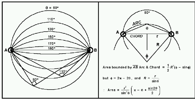
Figure 3: The geometry of the double-lobe background calculation

The ‘static’ background comes from considering random pairs of radio detections around an optical object. We should of course expect to see equal numbers of sources for all radio-optical-radio angles. This background of random configurations dominates our set of candidate lobes. The ‘geometric’ background consists of false optical matches to true double lobes, and is modelled by considering random optical objects within a disk bounded by two lobes at opposite ends, which contains the entire space for all angles $\geq 90^{\circ}$; Fig. 3a shows that each angle ($\theta$) space follows an arc which passes through both lobes A and B, and Fig. 3b shows that the arc is of a notional circle of radius $R=r/sin\theta$ where r is half the distance between the two lobes. An individual angle space (e.g. $\theta=163\degr$) can be quantified by using the area of the segment of disk R bounded by the arc and chord connecting the two lobes, as shown in Fig. 3b (where $\theta$ is expressed in radians); the angle space area of e.g. $163\degr$ is the difference in areas of the disk segments defined by $\theta=162.5\degr$ and $\theta=163.5\degr$. In this way it can be shown that the normalized expectation of finding a false lobe configuration per individual angle (e.g. 163°) ranges from 200% of mean at $90\degr$ to 66.67% of mean at $180\degr$, and has the form

$$e(\theta)=180 \times \left[{{1-(\theta-.5)/180+\sin(2(\theta-.5))/2}\over{\sin^{2}(\theta-.5)}}\right.$$ (8)

$$-\left.{{1-(\theta+.5)/180+\sin(2(\theta+.5))/2}\over{\sin^{2}(\theta+.5)}}\right]$$

$$(90\degr\leq\theta<179.5\degr)$$

The level of the geometric background cannot be estimated in isolation as it depends on the presence of all true lobes, including those for which the true optical identification is too faint to be found in our optical catalogue. We choose to combine estimates of the static and geometric background in such a way as to yield an angle-based excess corresponding to our expectation that there will be few lobes with angles of $<140^{\circ}$, with lobes increasing as we approach 180°. The decisive constraint is that the excess lobe population should be small and flat between $110\degr$ and $140\degr$, so we find static and geometric populations which will match that expectation. In practice this constraint imposes a delicate balance between the two populations, and we consequently find that per single- angle bin (e.g., 167°) of the FIRST lobe candidates the static background value is about 6475 objects and the geometric background has a coefficient multiplier of about 500 for equation (4). Similarly, 17000 and 2700 are the static and geometric per-angle values found which suit NVSS, and 1300 and 215 are found for SUMSS. These values, accumulated into $5\degr$ angle bins, yield the excess above background shown in Table 11.

Table 13: Double-lobe excesses derived for the three radio catalogues, binned by $5\degr$ angles (180° is half-width). Columns are the ‘double lobe candidates’ based on all the permutations of double-radio and single- optical configurations within disks of sky of 90 arcsec radius, the static random background and geometric background derived from our fit coefficients, and the residual excess after background subtraction. ‘Best unique’ lobe numbers are reductions by the quantified criteria (CLA etc), yielding unique candidate counts for each $5\degr$ bin. The values of ‘Ratio used’ are generated by the angle formulae from Table 12.

		Double lobe	Static	Geometric		Best	Excess/	Ratio
Survey	Angle (°)	candidates	background	background	Excess	unique	unique	used
FIRST	115	35323	32375	2868	80	4985	0.016	0.008
FIRST	120	35081	32375	2638	68	5210	0.013	0.010
FIRST	125	34892	32375	2445	72	5482	0.013	0.014
FIRST	130	34581	32375	2282	-76	5710	$-$0.013	0.019
FIRST	135	34784	32375	2146	263	6029	0.044	0.027
FIRST	140	34646	32375	2035	236	6333	0.037	0.036
FIRST	145	34659	32375	1940	344	6467	0.053	0.050
FIRST	150	34447	32375	1862	210	6870	0.031	0.069
FIRST	155	34984	32375	1801	808	7234	0.112	0.094
FIRST	160	35211	32375	1751	1085	7607	0.143	0.129
FIRST	165	35588	32375	1713	1500	8134	0.184	0.176
FIRST	170	36185	32375	1687	2123	8456	0.251	0.242
FIRST	175	37842	32375	1672	3795	9299	0.408	0.331
FIRST	180(hw)	19051	16188	750	2113	4773	0.443	0.453
NVSS	115	99657	85000	15492	-835	10066	$-$0.083	0.003
NVSS	120	98872	85000	14242	-370	10791	$-0.034$	0.004
NVSS	125	98290	85000	13198	92	11232	0.008	0.005
NVSS	130	97377	85000	12325	52	11914	0.004	0.007
NVSS	135	96507	85000	11594	-87	12542	$-0.007$	0.010
NVSS	140	96060	85000	10983	77	13268	0.006	0.014
NVSS	145	95824	85000	10475	349	13764	0.025	0.020
NVSS	150	95999	85000	10057	942	14509	0.065	0.029
NVSS	155	95607	85000	9722	885	15277	0.058	0.041
NVSS	160	95804	85000	9454	1350	15923	0.085	0.057
NVSS	165	95820	85000	9254	1566	16640	0.094	0.081
NVSS	170	96127	85000	9113	2014	17486	0.115	0.115
NVSS	175	96830	85000	9031	2799	18011	0.155	0.162
NVSS	180(hw)	48587	42500	4050	2037	9382	0.217	0.230
SUMSS	115	7756	6500	1234	22	579	0.038	0.003
SUMSS	120	7550	6500	1134	-84	655	$-0.128$	0.005
SUMSS	125	7566	6500	1050	16	737	0.022	0.007
SUMSS	130	7569	6500	981	88	811	0.109	0.010
SUMSS	135	7428	6500	923	5	850	0.006	0.014
SUMSS	140	7412	6500	875	37	887	0.042	0.020
SUMSS	145	7488	6500	834	154	1053	0.146	0.028
SUMSS	150	7339	6500	801	38	1073	0.035	0.039
SUMSS	155	7305	6500	775	30	1117	0.027	0.056
SUMSS	160	7430	6500	753	177	1186	0.149	0.079
SUMSS	165	7535	6500	736	299	1322	0.226	0.111
SUMSS	170	7375	6500	725	150	1395	0.108	0.157
SUMSS	175	7549	6500	719	330	1466	0.225	0.222
SUMSS	180(hw)	3754	3250	322	182	763	0.239	0.314

Table 11 shows the static and geometric background figures that we subtract from the total number of possible candidate lobes to yield the excess of lobe candidates above the background expectation. The excess totals to about 12000 for FIRST, 12000 for NVSS and 1500 for SUMSS, so these are approximately the numbers we’ll be trying to locate. The next column, ‘best unique’, gives the number of best unique lobes identified by the lobe selection criteria. Our task is to find which of these best unique candidates are the genuine lobes enumerated by the excess. The next column ‘excess/unique’ shows the fraction of the best unique candidates that we expect will be genuine lobes. The last column is the per-angle value of the formula (shown in Table 12) that we design to simulate the ratio. This formula is applied to the angle of each candidate double lobe as an absolute starting point; thus, for example, a FIRST candidate with angle of 152° is assigned the angle-based expectation of 0.0777, since we nominally expect 7.77% of these objects to be true lobes. Our final score for each double-lobe candidate will be on an open-ended scale normalized to a score of 1 equating to a 50% probability of being a lobe, i.e. score = odds/(1-odds). So we first convert our angle-based expectation into that scale, so 0.0777 becomes 0.0777/(1-0.0777) = 0.0843. For this candidate now to attain a final 50% score it will need to gain a total multiplier of 11.9 from the other six selection criteria all of which have had curve-fitting formulae similarly constructed as above, but are normalized to 1 equating to 50%. These formulae for the seven quantified criteria, displayed in Table 12, are only heuristic data-curve fitters and do not have any physical meaning. The importance of fitting curves closely was brought home to us when we initially derived curve-fits for only the FIRST catalogue and applied them to the NVSS: results were sparse. So we have elected to prefer exactitude over simplicity in designing these formulae, but we emphasise that they are just heuristic estimators.

Table 14: Formulae used to calculate quantitative criteria to evaluate candidate double lobe configurations.

Criterion	FIRST formula	NVSS formula	SUMSS formula	Notes
Angle ($\theta$)	$2^{(\theta-156)/11}/10$	$2^{(\theta-158)/10}/20$	$2^{(\theta-155)/10)}/18$
Distpct ($\delta$)	$1+(\delta-65)/90$	$1+(\delta-62)/62$	$1+(\delta-62)/62$
SNRpct ($R$)	$2^{(R/45)-1}$	$2^{(R-62)/12}$	$2^{(R-75)/12}$	eq 0.5 if $S=100$ (sidelobe)
SDratio ($S$)	$2^{\log_{2}(S)-6}$	$3^{\log_{2}(S)-5.2}$	$4^{\log_{2}(S)-4.2}$	max 35
CLA ($\psi$)	$5^{(1-\psi/35)}$	$4.2-\psi/9$	$3.5-\psi/15$	min 0.15, max 3 for FIRST
EA ($E$)	$1.75+E/2$	$1.33+E/1.33$	$0.5+E/2$	0.33 if $E=0$, max 25
Offset ($\Delta$)	$2^{(31-\Delta)/6}$	$2^{(46-\Delta)/12}$	$2^{(54-\Delta)/6}$	min 0.1, max 1

As an example of how these formulae were derived, the data which yielded the CLA formulae are presented in Table 13. ‘Best’ candidates are compared to all candidates. A ‘best’ candidate is one which scores above the mean for each of all the other criteria, and so is double-lobe-like in every way. We conjectured that these well-behaved candidates were true lobes and so used them as a control population (we confirmed that more than 95% of them were likely lobe detections by inspection of images from the surveys). We derived the ratio of these best candidates to all the candidates for each CLA value binned by 5°, and normalized this about the mean. The last column for each survey is the formula-derived score, using that survey’s CLA formula from Table 12 which replicates the normalised ratio. Thus the cumulative effect of applying these scores to the data is that the total score is approximately unchanged.

Table 15: Comparative Lobe Angle dependent attributes of the input radio catalogues.

	FIRST	FIRST	normal	FIRST	NVSS	NVSS	normal	NVSS	SUMSS	SUMSS	normal	SUMSS
CLA	best	backgd	ratio	calc	best	backgd	ratio	calc	best	backgd	ratio	calc
0(hw)	90	17403	3.57	3.00	45	49684	4.94	4.20	5	2356	3.17	3.50
5	153	35087	3.01	3.00	74	99889	4.04	3.64	9	4665	2.88	3.17
10	137	34753	2.72	3.00	62	98794	3.42	3.09	17	4754	5.34	2.83
15	128	34921	2.53	2.51	45	98635	2.49	2.53	4	4711	1.27	2.50
20	104	34733	2.07	1.99	28	98228	1.56	1.98	5	4700	1.59	2.17
25	85	34547	1.70	1.58	33	98125	1.84	1.42	5	4683	1.59	1.83
30	54	34543	1.08	1.26	16	98174	0.89	0.87	6	4714	1.90	1.50
35	48	34397	0.96	1.00	5	98194	0.28	0.31	3	4778	0.94	1.17
40	26	34640	0.52	0.79	3	98105	0.17	0.15	1	4707	0.32	0.83
45	31	34368	0.62	0.63	5	98206	0.28	0.15	1	4722	0.32	0.50
50	17	34572	0.34	0.50	3	97806	0.17	0.15	1	4539	0.32	0.17
55	12	34624	0.24	0.40	4	98020	0.22	0.15	.	4871	.	0.15
60	14	34687	0.28	0.32	2	98461	0.11	0.15	.	4750	.	0.15
65	5	34828	0.10	0.25	.	98511	.	0.15	.	4651	.	0.15
70	.	34867	.	0.20	.	98254	.	0.15	.	4729	.	0.15
75	.	34813	.	0.16	.	99331	.	0.15	.	4817	.	0.15
80	.	34685	.	0.15	.	98455	.	0.15	.	4717	.	0.15
85	.	34616	.	0.15	.	99380	.	0.15	.	4805	.	0.15
90(hw)	.	17257	.	0.15	.	49372	.	0.15	.	2456	.	0.15

Each double-lobe candidate is scored using the seven criteria, and the individual scores are multiplied together to give the total normalized score for the candidate, so a total score of 1 indicates that the candidate is about 50% likely to be a lobe. Since the starting score from the angle-based excess is of the order of 0.1, it is clear that a lobe candidate will need to pick up good scores from a number of these criteria to achieve a high score, signifying a true lobe. We also use two additional normalized criteria which aid in choosing an optical source for a double lobe where there are multiple optical candidates: (1) Core radio detection: An optical candidate directly detected in radio is a very strong source candidate for suitably configured lobes. We have quantified this as a 15x multiplier via analysis against ‘best’ candidates similar to that presented for CLA, above. (2) Optical morphology and colour: This quantifies which types of optical objects are most likely to be associated with radio lobes, gauged again by analysis of the data as with CLA. Objects absent in one colour are only one-third as likely to be radio emitters, and objects stellar in red are two-thirds the likelihood. Objects that are non-stellar in red, i.e. galaxies, are 2.25 times as likely to be the core object. Blue colour morphology is weighted as for the red colours but with half the significance. Colours (B-R) impact the final likelihood in a range from .33x to 3.5x; in the case of stellar objects it is the blueish objects which are favourable and the reddish unfavourable, whilst with galaxies it is the reverse. These two centroid- based multipliers are removed after de-duplication, so do not contribute to the final score on which the lobe-ness of the candidate is assessed. One artefact which caused us some trouble was that some sidelobes still remain unflagged in the source catalogues; these appear as regularly- spaced spikes ringing bright sources and so score quite well on some of our tests, but their very regular nature allows us to trap and remove them with some success, as with perfectly matched SNRpcts on Table 12 where we assign a low score. We also removed pairs with very faint SNRs where the ellipses were perfectly round – this too denoted sidelobes.

When all two-radio-one-optical candidate scoring has been completed, all candidates scoring less than 33% are discarded and the rest are de- duplicated by peeling off the top; that is, accepting the top-scoring combinations and then removing any other candidates that were sharing those radio or optical objects, and repeating to completion. Thus we are left with completely unique two-radio-one-optical candidates with final probability scores. To clarify the status of low-scoring candidates we found it useful to apply our standard likelihood algorithm treating the lobes as highly-offset core detections; the average density score at high offsets is 1 (= background), but for some optical PSFs and colours it is greater than 1 and for others less, so the likelihood algorithm confers an additional judgement on whether that class of centroid typically shows large-offset associations above the background, i.e., lobes. Thus our last step to these lobe probability calculations is to add the likelihood density to the lobe probability score and treat this final score as a likelihood density figure so that a density of 2 equates to a confidence of 50% using equation (2), etc. We apply a cutoff at confidence=40% and the surviving double-lobe candidates are accepted for inclusion into our catalogue. Comparison of our results with images from the radio surveys shows our results to be in good agreement with the radio images, i.e. where our catalogue says we find lobes, they generally do look like lobes.

To check our results more stringently, we compare them with a radio survey with pre-existing optical identification, the online 3CRR catalogue (Laing, Riley & Longair 1983) at http://www.3crr.dyndns.org/ . Because this is a low-frequency flux density selected sample, it contains the brightest lobes; as these are often large and nearby, we do not expect to detect all of the lobes given our size limit of 90 arcsec. However, there are few radio source surveys with a high enough identification fraction to meet our needs. We considered using the $z\sim 1$ B2/6C ‘Distant DRAGNs’ survey (Eales et al. 1997), in which the lobe sizes are generally smaller, but of their 27 IR-detected centroids only two are bright enough in V to appear in our optical catalogue! As it happens, both centroids (0901+35 and 1045+35A) have double lobes of LAS $<8$ arcsec so that FIRST reports them as single detections only and so appear in our catalogue as core-detected objects QORG J090432.3+353904 and QORG J104830.4+353801. Of Eales’ remaining double lobes, one pair (0905+39) is declared in QORG associated at 85% confidence to a nearby (23 arcsec) false centroid QORG J090818.8+394319, and the remainder are excluded due to the absence of any suitable optical objects. This result gives a sense of the optical faintness of $z\sim 1$ galaxies which are not optically selected, and is encouraging in the sense that there was only one QORG assignation of double lobes to a false centroid where 14 double lobes (and 12 core detections) are seen in the FIRST data.

Returning to the 3CRR catalogue, it lists 173 optical identifications, of which 13 are core detections only, for which inspection of FIRST/NVSS reveals 80 core (offset $\leq 3$ arcsec) radio detections and $\sim 90$ possible lobe pairs within 90 arcsec of the centroids. However only 132 of the 173 centroids appear in our optical data copositioned within 8 arcsec of the listed 3CRR position, and of these, 10 have no core radio detection nor more than one FIRST/NVSS radio signature within 90 arcsec. Of the remaining 122 optical centroids we find our catalogue has associated 62 to core radio detections; 8 additional core detections were rejected by our likelihood algorithm as they are astrometrically offset too far from the optical centroids. Also for these 122 optical 3CRR centroids, inspection of FIRST/NVSS reveals $\sim 70$ possible lobe pairs within 90 arcsec from which our QORG algorithm identified 58 lobe pairs and associated 43 of these with optical objects that we here find are the correct 3CRR centroids for a 74% hit rate on double- lobe declarations; about 6 more were associated with optical signatures within 20 arcsec of the 3CRR centroids which look possibly related. Given that FIRST tends to break these large, bright lobes down into multiple ellipses, we feel that our algorithms have performed reasonably here. In all, 102 out of the eligible 122 optical 3CRR centroids are radio- associated in our catalogue. The complete list of the 3CRR centroids and our results for them is viewable at http://quasars.org/docs/3CRR-QORG.txt, which also displays confidence percentages for those near-core radio- optical superpositions which were rejected. In the QORG catalogue we have retained, for consistency, those objects that this exercise has shown to be false centroids for 3CRR double lobes, but we have annotated some of these as ‘vicinity of’ a 3CRR centroid to identify the lobes to the user. This is a nod to our difficulty with lobes too large for our 90-arcsec selection criterion; we found no lobe candidates at all for the 8 3CRR galaxies listed with lobes of LAS$>1000$. However, such large sources are likely to be comparatively rare. The large bulk of QORG double-lobe declarations are for smaller lobes for which the centroid identification is usually straightforward, except where the true identification is too faint for our optical data, which is always a hazard. Table 14 gives a summary of lobe counts binned by angular size of the longer lobe.

Table 16: Summary of double radio lobe numbers in the QORG catalogue, by source catalogue and binned by angular size of the longer lobe in arcsec. Numbers of lobes, core detections, median lobe flux in mJy and median confidence of the QORG lobe declarations rounded to 1 per cent are displayed.

Ang size	FIRST				NVSS				SUMSS
longer	No.	No. core	median	median	No.	No. core	median	median	No.	No. core	median	median
lobe	double	det’ns	flux	conf	double	det’ns	flux	conf	double	det’ns	flux	conf
(arcsec)	lobes		(mJy)	(per cent)	lobes		(mJy)	(per cent)	lobes		(mJy)	(per cent)
2- 5	996	.	5	90	3	.	14	64	1	.	12	63
6-10	3142	196	5	96	19	1	6	63	3	.	111	67
11-15	2278	546	5	93	30	1	5	84	6	.	158	74
16-20	1531	385	5	93	37	.	10	77	9	.	255	92
21-25	1082	255	6	90	88	4	20	89	25	.	62	95
26-30	783	213	7	88	374	32	29	94	117	.	35	94
31-35	562	110	7	84	756	55	31	97	189	.	39	90
36-40	419	66	7	81	988	59	30	95	244	.	46	91
41-45	268	53	7	77	1032	53	28	92	237	.	40	90
46-50	160	30	8	75	1018	65	28	89	196	1	44	89
51-55	117	10	10	68	915	46	29	87	203	.	41	86
56-60	70	8	7	66	781	46	29	83	137	1	40	83
61-65	42	8	11	66	628	36	29	85	113	.	48	84
66-70	27	2	14	58	484	33	33	82	80	.	55	79
71-75	11	1	8	58	383	20	34	80	42	.	62	77
76-80	13	2	31	56	325	21	42	78	29	.	77	76
81-85	4	1	21	58	252	9	45	77	24	.	65	77
86-90	7	1	10	73	210	7	41	76	8	.	63	70
TOTAL	11512	1887	6	91	8323	488	30	88	1663	2	45	87

Table 14 shows that the 5-arcsec-resolution FIRST detections yield increasing lobe numbers at shorter angular size as expected from the increase in the background population with greater distance. NVSS and SUMSS have 45-arcsec resolution so at smaller angular sizes there is an increasing tendency for lobes to be merged into a single detection. Our total double lobe counts are seen to compare well with the calculated excesses from Table 11 (unsurprisingly, since those excesses provided our starting likelihood probabilities). For each individual double lobe candidate in the catalogue we list the nominal confidence percentage that it is a true double lobe with the stated optical centroid. Of course sometimes we select the wrong centroid, as seen in some 3CRR examples above, and some of our double lobe declarations are in fact unassociated and not double. There is necessarily some relation between our declared confidences and actual performance in discerning true lobes but in the absence of a large control sample we can only surmise that the relation is not too greatly skewed. Our total count of double lobe declarations is 21,498, of which about half are rated with a confidence over 90%, slightly over half for FIRST and slightly under half for NVSS & SUMSS.

In the end, the merit of our heuristic pattern detection algorithm for double radio lobes about optical centroids is weighed by its performance against the real sky. For the difficult, large 3CRR lobes we have achieved an accuracy of 74 cent per from a completeness of about 85 per cent against the FIRST/NVSS data. We expect better performance for the larger population of smaller lobes. We feel that our list of double lobe candidates over the whole sky, while not constituting a fully identified sample, gives the largest currently available sample of probable lobe identifications, and as such will be a useful resource for future research.

A.5 Use of the Identification Catalogues

The aim of our work has been to associate radio/X-ray detections with optical objects. The identification of an optical object as a known quasar, galaxy or star is important but secondary, in the sense that we do not wish to have to assess the level of our confidence that we have selected the correct optical signature. Accordingly we assign the identification only where we are essentially certain of it, which usually means astrometric alignment within 4 arcsec. The general method is that for each input identification catalogue we analyse offset annuli from the catalogued object positions to determine to what radius an optical population is found which is over twice the background; this is typically 4 arcsec for astrometrically accurate, recent catalogues. In most cases only a single optical object is found in our input catalogues within that radius, which we take as unambiguous identification; if no object is found then that identification is lost. Where there is more than one optical object within the radius we are content to use them all from then on, in the expectation that final selection of the correct object will come via one of them being found to be associated with a radio/X-ray source; where there is no radio/X-ray association the identification will not be used in our catalogue anyway. We modify these criteria when suited to a particular catalogue: for PGC galaxies we find that optical identification out to a 30 arcsec offset from the catalogued position is merited if the PSF is non-stellar, and for white dwarfs we find a maximum 15 arcsec offset if the PSF is stellar, as some of its data come from early surveys. Many identifications of course appear in many different catalogues, often with different names, so we have elected to use the earliest names available; thus we prefer galaxy names as given in the PGC as these are historical in nature. Where the PGC does not name a galaxy we use the earliest available name from another catalogue, and galaxies present only as a nameless entry in the PGC we write as e.g. PGC 12345, using the PGC number which is used by LEDA as an unchanging identifier. In the case of redshifts we wish to use the latest measured values as these are most likely to be accurate. Thus an identification in our catalogue will often get its name from one source and its redshift from another. Attributions for the names and redshifts are displayed in our catalogue for each identification, with the attribution references listed in the readme file; we give references only to source catalogues, and those catalogues should be consulted for information on the original identification.

Where an optical object is claimed by both a galaxy catalogue and a star catalogue we have set quality standards to decide between these, e.g. a recent redshift confirms an object as non-stellar, or a stellar PSF confirms a star identification over a galaxy identification without a redshift, etc. We have prepared a list of ‘interesting’ dual star/non- star identifications at http://quasars.org/docs/Star-NonStar-Duplicates.txt In this list we also flag when an object appears in our catalogue; it is only for those objects that our choice of the correct identification is important. In use of the QORG catalogue it is important to bear in mind that many such ‘stars’ have been misclassified, especially those from Tycho, HDx and GCVS which are not spectroscopically supported, and bright Tycho stars may conceal the actual sources of radio/X-ray emission. Thus any stellar identification, not already well-understood, that is reported in our catalogue to be associated with a radio/X-ray detection, should be considered suspect, especially for those few that are nominally associated with double radio lobes.

A key identification in this catalogue is that of catalogued QSOs and BL Lacs; we identify these with optical objects even in the absence of a radio/X-ray association. We do this since QSOs are such significant objects, and since they are all likely to be X-ray and (in the case of BL Lacs at least) radio emitters whether we have detected them or not We are content to rely on the Veron catalogue as the arbitrator of QSO identification, so we exclude objects identified elsewhere (e.g. CfA) as QSOs which are absent from Veron, unless included by radio/X-ray association. Our faith in the judiciousness of the Veron catalogue is partly prompted by that one of us (EF) has assisted in tidying up problem areas in its recent releases, so we have some personal knowledge of its strengths. We endeavour to optically locate QSOs however practical. Most QSOs, especially the large number recently identified in SDSS and 2QZ surveys, are unambiguously identified with isolated optical objects within the usual 4-arcsec astrometric radius. We have used these unambiguous QSO- optical matches to construct a qualitative QSO optical profile which we then apply to those cases where an identified QSO has multiple nearby optical candidates; this plus magnitude comparison, plus a subset of unambiguous ROSAT/radio detection locations, allows us to select a superior optical candidate in nearly all cases. As a tiebreaker between two equally good candidates (which is rare) we simply select the nearer one. For a QSO listed with a magnitude near or below our plate depth, if there is no faint optical candidate within 4 arcsec we discard that QSO as being undetected.

A special case in QSO identification is that of the older QSO surveys of the 1980s and 1990s as listed in the Veron catalogue. These are often listed with significantly discrepant astrometry and photometry making computerized identification problematic. We have found that the discrepancies often appear to have a systematic component peculiar to each original survey. Thus we find, for each original survey, the astrometric and photometric offsets to our optical catalogue for those (often few) unambiguous identifications, and then applying those offsets to all that survey’s QSOs and then re-matching to our optical catalogue, repeating in an iterative process until stability is reached. This can result in unambiguous recovery of many or most of the optical objects matching those QSOs, and we also use the above-mentioned qualitative profile to find most-likely optical candidates offset up to 40 arcsec. In this way we have assisted our recovery of about 200 QSO-optical identifications for the old surveys, confirmed by comparison of a large subset to the original finding charts, which we accordingly include in QORG with an astrometric and photometric accuracy not found elsewhere. Surveys thus given interesting shifts are displayed at http://quasars.org/docs/Personal-Equation.txt, although we leave off those QSOs that were subsequently re- surveyed, for which updated information is available in the latest version of the Veron catalogue.

Table 15 summarizes the identification catalogues contributing to QORG. The CfA Redshift catalogue is itself a compendium of many catalogues and papers, and includes the main LBQS and LCRS data leaving us to add in those residual star identifications separately. The CfA, NED, White Dwarf, PGC and Veron catalogues are collections of heterogeneous data which have been standardized somewhat by those catalogues’ authors whilst retaining historical names; the other catalogues are more internally consistent and often derived from single surveys. Use of name and positional information directly from the large SDSS and 2QZ catalogues allows consistent presentation across different object types, which we prefer over the short forms used in the Veron catalogue. Where we use the name of an object we also use its type (quasar, galaxy etc.) supplied by that catalogue except that we use any Veron-supplied type. Many catalogues categorize galaxies into subtypes like NELGs, but such distinctions are unclear for many galaxies and heterogeneously applied across catalogues, so we thought it cleaner to simply defer to the Veron categorization of some galaxies as AGN and leave the rest annotated just as ‘galaxies’. Thus we show just five identification types in QORG: 49743 galaxies, 48285 quasars, 14633 AGN, 6314 stars and 841 BL Lacs. There are also 91 objects listed as ‘U’ for unidentified, where a redshift or other information is displayed. We include into QORG all QSOs, AGN and BL Lacs for which we find an optical object; the others require a radio/X-ray association for inclusion. Note that the LBQS stars data contain one BL Lac identified in the original paper which was inadvertently left off their catalogue (P. Hewett, private communication); it is included in our catalogue.

Table 17: Identification catalogues. See the ‘source catalogues’ section for full attributions. Types of objects identified in each catalogue are listed in order of their numerical prevalence: Q=QSO, A=AGN, B=BL Lac, G=galaxy, S=star, U=unknown. The total used for names in QORG includes all identified objects plus 91 unknown objects bearing names.

	Object	Total no.	No. used	No. used
	types	unique	for name	redshift
Catalogue	incl	objects	in QORG	in QORG
2dFGRS	GS	236078	3403	2916
2QZ	QSABGU	40439	22077	22019
3CRR	GQA	173	49	43
6dF	G	15035	663	853
6QZ	SQABG	1529	261	265
CfA	GQABS	234703	2564	6432
Common Names	S	1127	173	–
CV	S	1143	184	–
ENEAR	G	1174	12	25
GCVS	S	10553	146	–
HDx	S	88831	200	–
LBQS stars	SB	1390	1	–
LCRS stars	S	886	2	–
NED	(all)	(lots)	52	52
NLTT	S	71663	235	–
PGC (LEDA)	G	1088795	38611	1250
PSCz	GS	15423	301	811
SDSS	GSQU	181959	23282	20209
Tycho	S	2539737	4871	–
UGC	G	13390	37	267
Veron	QABSGU	64942	22404	27536
White Dwarfs	S	2206	97	–
Yale	S	3131	204	–
Zwicky	G	19372	78	2958
TOTAL	SGQABU		119907	85636

In all, we have tried to include all computer-processable identifications extant in the literature to provide a fully annotated picture of the known radio/X-ray (ROSAT) sky. We use these identifications to calculate odds that unidentified radio/X-ray objects are in turn quasars, galaxies or stars, as explained in the main section of this paper.

A.6 Attributes of this Catalogue

A.6.1 De-duplication and identification

After construction of the catalogue we found it necessary to perform some de-duplication because of large bright objects such as plate-saturating stars or large galaxies with multiple components which manifest as multiple optical signatures; these attract associations from multiple ROSAT fields where in fact both X-ray sources and optical signatures are just duplicates. To allow this situation to go uncorrected would diminish the ease of use of the catalogue and possibly mislead the user. About 1500 such duplicates across different ROSAT fields have been removed or amalgamated via preferential retention of associations to the bright central star or galaxy, while closely adjacent associations within the same ROSAT field are preserved. The radio surveys have a separate issue that resolved FIRST double lobes are often presented by the NVSS as a single central source, which would constitute a false core detection if left unattended; we have removed the NVSS association in those cases, which number about 750. These de-duplications have clarified cases of multiple associations across radio and X-ray catalogues, and condensed our catalogue by about 0.5%.

We have made an adjustment to the likelihood-of-association probabilities as one of the last acts of writing this catalogue. Small numbers variations in the density calculations have occasionally resulted in large densities at up to 30 arcsec offset, and at large offsets it is also common to encounter multiple optical candidates which would decrease the odds of association for any one of them. We have attached an additional likelihood penalty to far-offset associations to take account of the increased presence of multiple candidates. We used a simple rule of thumb for offsets greater than 6 arcsec, subtracting 1/6 density point for each additional arcsec offset, e.g. at 9 arcsec 2.3 becomes 1.8. This dampens high-offset densities to where 21 arcsec is the furthest offset for any $>70$% confidence association presented, and 26 arcsec for any at all. To put this in perspective, 95% of all our presented core associations are offset within 8 arcsec, and 75% are within 4 arcsec. This may be a conservative measure, but we feel it is more excusable to under-represent true far-offset associations than it is to over-represent false ones.

A.6.2 Distribution on the sky

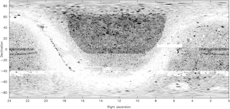
Figure 4: A whole-sky optical density map (as Fig. 1) showing only those 449,309 objects in our catalogue which are associated with radio/X-ray detections.

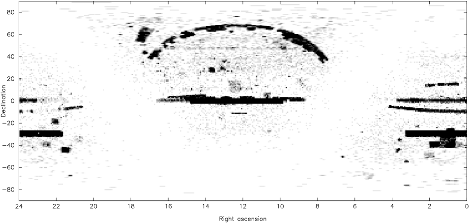
Figure 5: A whole-sky optical density map (as Fig. 1) of the 53,930 catalogued QSOs (including BL Lacs and stellar-PSF AGN) found in our catalogue.

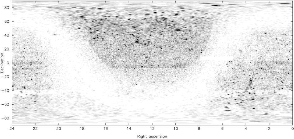
Figure 6: A whole-sky optical density map (as Fig. 1) showing all 86,009 objects in our catalogue, not currently identified, which we list as being 40% to $>99$% likely to be a QSO.

Because of the properties of the catalogues from which they originate, the identified sources are not entirely uniformly distributed on the sky. Fig. 1 is a whole-sky optical density map of all 501,761 objects presented in the QORG catalogue. In the North galactic cap (NGC) the large dense area in the centre is the FIRST survey area, the dense equatorial strip is the part surveyed by both SDSS and 2dF, and the crescent-shaped area to the North was surveyed by the SDSS first release. In the SGC, the straight equatorial strip and the curved strip below it are the FIRST south-sky survey area, the dense straight area below that is 2dF-surveyed, and the white strip below that is the part of the sky not surveyed in radio, with NVSS-surveyed areas to the north and SUMSS to the south. The dense strip in the Galactic dust lane to the East (left) shows an artefact of our likelihood method where likely Galactic sources of radio/X-ray emission are being presented as likely extragalactic; we have retained these nominal associations in case some should prove useful, but users are cautioned that probably most are spurious. In Fig. 4 we show a similar density map showing only those 449,309 objects in our catalogue which are associated with radio/X-ray detections. The SDSS and 2dF survey bands are missing from this map as they are identification surveys, not radio/X-ray surveys. It can be seen that the density of the radio/X-ray sources is quite uniform; the main effect on the density, apart from the Galactic plane, is the area covered by FIRST.

Turning to QSOs, Fig. 5 is an all-sky density map of the 53,930 catalogued QSOs (including BL Lacs and stellar-PSF AGN) found in our catalogue. It can be seen that 3/4 of them are concentrated into the recent SDSS and 2QZ survey areas, and the remainder are inhomogeneously distributed, showing how incomplete the overall QSO enumeration has been to date. By contrast, Fig. 6 is a similar density map showing all 86,009 objects in our catalogue, not currently identified, which we list as being 40% to $>99$% likely to be a QSO. It can be seen that these are arrayed fairly uniformly on the sky, barring the Galactic plane and the zone of declination $-45\degr$ which is as yet unsurveyed in radio.

A.6.3 AGN properties

We must necessarily begin this section of the discussion with a caveat. Because the properties of the newly identified objects in our catalogue are determined in a probabilistic way from the properties of existing objects, it is dangerous to consider the statistics of the newly identified objects and try to derive from them new results about the population of X-ray and radio-identified optical objects as a whole. For example, Fig. 7 shows plots of $R$ against $B$ magnitude for the previously identified and previously unidentified sources in the sample, divided by object identification class. It will be seen that the new sources lie in somewhat different areas of parameter space (so, for example, there are few newly identified galaxies with $R<15$, simply because the vast majority of resolved objects with these magnitudes are already in catalogues). But the important point is that the identification algorithm in general populates a subset of the areas delineated by the existing data. It cannot, by its nature, tell us more about the distribution of sources with particular identifications in parameter space than the original identification catalogue on which it was based.

With this in mind, it is worth carrying out a few simple analyses of the characteristics of the objects in the catalogue. We begin by examining the relationship between X-ray flux and optical magnitude (Fig. 8). The previously identified sources fall into clear regions of parameter space; it is of course no surprise that for a given X-ray count rate stars are generally optically brighter than galaxies and galaxies brighter than quasars. The newly identified objects adopt similar regions of parameter space, as expected, although there is a relatively greater number of optically and X-ray faint objects. The sharp line between galaxies and stars seen in the newly identified objects is likely to be in part an artefact of the way that radio/X-ray ratio is taken into account by the classification algorithm (Section A.6). At the optically faint end, the probabilities that a given object is a quasar or a galaxy are similar – this reflects the difficulty in making a clear distinction between the two types of object at faint magnitudes. We note that a ROSAT PSPC count rate of $\sim 10$ h^-1 corresponds to around 40 Chandra counts in 5 ks, and thus the types of sources being identified here should be routinely found in Chandra and XMM observations as (soft) serendipitous sources.

The corresponding radio plots (Fig. 9) are also consistent with expectation. Identifications with galaxies are most probable at small magnitudes; quasars appear in large numbers above $R\sim 16$, as seen in other catalogues, and above this magnitude the numbers of galaxy and quasar identifications are similar, as expected from unified models. As with the X-ray sources, the plot of newly identified radio sources shows a higher density of galaxies at $R\sim 20$ than is seen in the identified sample.

A small number of objects (5,325 galaxies and QSOs and a handful of objects classified as stars, all at the $>40$% level) are identified as both radio and X-ray sources. While the QSOs show a clear trend in the sense that X-ray count rate and radio flux density are correlated, there is little evidence for a correlation between these quantities for sources identified as probable galaxies. These are likely to be more heterogeneous sources, including starbursts as well as radio galaxies in a variety of environments. A trend in the same sense is also present for sources with detected radio lobes and X-ray counterparts, the vast majority of which are identified with quasars.

Figure 7: $B$ against $R$ magnitude for (top) the previously identified sources and (bottom) the newly identified sources in the catalogue. Density of red, green and blue points represent density of sources identified in the catalogue as galaxies, stars and quasars respectively (only $>40$% confidence identifications are used). Colours are additive in RGB colour space, so, for example, a magenta region on the plot represents a high density of both quasars and galaxies. Note that stars are over-represented for visibility.

Figure 8: ROSAT count rate (the mean of all available count rates, with the HRI value scaled up by a factor 3 to bring it in line with the PSPC values) against $R$ magnitude for (top) the previously identified sources and (bottom) the newly identified sources in the catalogue. Colours as for Fig. 7. The top figure contains 13,733 data points, the bottom one 60,661.

Figure 9: 1.4-GHz total flux density, including lobes where detected, from FIRST and NVSS, against $R$ magnitude for (top) the previously identified sources and (bottom) the newly identified sources in the catalogue. Colours as for Fig. 7. The top figure contains 52,995 data points, the bottom one 274,505. Quasars are over-represented for visibility.

References

- (1) Abazajian, K., Adelman, J., Agueros, M., et al., 2003, AJ, 126, 2081
- (2) Bade, N., Engels, D., Voges, W., Beckmann, V., Boller, Th., Cordis, L., Dahlem, M., Englhauser, J., Molthagen, K., Nass, P., Studt, J., Reimers, D., 1998, A&AS, 127, 145
- (3) Barcons, X., et al., 2002, A&A, 382, 522
- (4) Bock, D. C.-J., Large, M. I., Sadler, E. M., 1999, AJ, 117, 1578
- (5) Colless, M., et al., 2001, MNRAS, 328, 1039
- (6) Condon, J. J., Cotton, W. D., Greisen, E. W., Yin, Q. F., Perley, R. A., Taylor, G. B., & Broderick, J. J., 1998, AJ, 115, 1693
- (7) Cotton W.D., Condon J.J., 1999, ApJS, 125, 409
- (8) Croom S.M., Smith R.J., Boyle B.J., Shanks T., Miller L., Outram P.J., Loaring N.S., 2003, MNRAS, submitted
- (9) Downes, R. A., Webbink, R. F., Shara, M. M., Ritter, H., Kolb, U., Duerbeck, H. W., 2001, PASP, 113, 764
- (10) Eales, S., Rawlings, S., Law-Green, D., Cotter, G., Lacy, M., 1997, MNRAS, 291, 593
- (11) Falco E.E., Kurtz M.J., Geller M.J., Huchra J.P., Peters J., Berlind P., Mink D.J., Tokarz S.P., Elwell B., 1999, PASP, 111, 438
- (12) Gould, A., 2003, AJ, 126, 472
- (13) Hewett P.C., Foltz C.B., Chaffee F.H., 1995, AJ, 109, 1498
- (14) Hoffleit E.D., Warren Jr. W.H., 1991, The Bright Star Catalogue, http://cdsweb.u-strasbg.fr/cgi-bin/Cat?V/50
- (15) Hog et al., 2000, A&A, 355, 27
- (16) Huchra, J. P., Geller, M. J., Clemens, C. M., Tokarz, S. P., Michel, A. 1999, ApJS, 121, 287 (http://cfa-www.harvard.edu/ huchra/zcat)
- (17) Kim, D.-W., et al., 2004, ApJS, 150, 19
- (18) Laing R.A., Riley J.M., Longair M.S., 1983, MNRAS, 204, 151
- (19) Mason, K. O., et al., 2000, MNRAS 311, 456 (RIXOS)
- (20) Mauch, T., Murphy, T., Buttery, H. J., Curran, J., Hunstead, R. W., Piestrzynski, B., Robertson, J. G., Sadler, E. M., 2003, MNRAS 342, 1117
- (21) McMahon, R. G., Irwin, M. J., 1992, in Digitised Optical Sky Surveys, eds. H. T. MacGillivray and E. B. Thomson (Dordrecht: Kluwer), p. 417
- (22) McCook G.P., Sion E.M., 1999, ApJS, 121, 1
- (23) McMahon, R. G., White, R. L., Helfand, D. J., Becker, R. H., 2002, ApJS, 143, 1
- (24) Monet, D., Canzian, B., Harris, H., Reid, N., Rhodes, A., Sell, S., 1997, USNO-A1.0 (http://archive.ast.cam.ac.uk/viz-bin/VizieR?-source=I/243)
- (25) Monet, D., et al., 1998, USNO- A2.0, http://archive.ast.cam.ac.uk/viz-bin/VizieR?-source=I/252
- (26) Monet, D., et al., 2003, AJ, 125, 984 (USNO-B)
- (27) Murray, C. A., 1989, A&A, 218, 325
- (28) Nesterov V.V., Kuzmin A.V., Ashimbaeva N.T., Volchkov A.A., Roeser S., Bastian U., 1995, A&AS, 110, 367
- (29) Paturel, G., Bottinelli, L., Gouguenheim, L., 1995, ApL&C, 30, 13
- (30) Samus, N.N., et al., 2002, Ast. Lett., 28, 174
- (31) Saunders, W., et al,. 2000, MNRAS, 317, 55
- (32) Schneider, D.P., et al., 2003, AJ, 126, 2579
- (33) Shectman, S.A., Landy, S.D., Oemler, A., Tucker, D.L., Lin, H., Kirshner, R.P., Schechter, P.L. 1996, ApJ, 470, 172
- (34) Salim, S., Gould, A. 2003, ApJ, 582, 1011
- (35) Smith, W.B., 1996, The Common Name Cross Index, http://xml.gsfc.nasa.gov/pub/adc/xml_archives/catalogs/4/4022/
- (36) Véron-Cetty, M.-P., Véron, P. 2003, A&A, 412, 399
- (37) Voges et al. 1999a, A&A, 349, 389
- (38) Voges, W. et al. 1999b, in Diffuse thermal and relativistic plasma in galaxy clusters, H. Bohringer, L. Feretti, P Schuecker, eds., Max-Planck-Institut für Extraterrestrische Physik, Garching, p. 179.
- (39) Voges et al. 2000, ROSAT All-Sky Survey Faint Source Catalogue, http://www.xray.mpe.mpg.de/rosat/survey/rass-fsc/
- (40) Wakamatsu, K., Colless, M.M., Jarrett, T., Parker, Q., Saunders, W., Watson, F. 2002, IAU Regional Assembly, ASP Conf. Proc., in press
- (41) Wegner, G., et al., 2003, AJ, 126, 2268
- (42) White, N.E., Giommi, P., Angelini, L. 1994 AAS 185, 4111
- (43) White, R. L., et al. 2000, ApJS, 126, 133
- (44) White, R.L., Becker, R.H., Helfand, D.J., Gregg, M.D. 1997, ApJ, 475, 479
- (45) XMM: the first XMM-Newton Serendipitous Source Catalogue, XMM-Newton Survey Science Centre (SSC), 2003, is accessible at http://xmmssc- www.star.le.ac.uk/