SPECTRAL MODELLING OF STAR-FORMING REGIONS IN THE ULTRAVIOLET: STELLAR METALLICITY DIAGNOSTICS FOR HIGH REDSHIFT GALAXIES

Abstract

The chemical composition of high redshift galaxies is an important property which gives clues to their past history and future evolution and yet is difficult to measure with current techniques. In this paper we investigate new metallicity indicators, based upon the strengths of stellar photospheric features at rest-frame ultraviolet wavelengths. By combining the evolutionary spectral synthesis code Starburst99 with the output from the non-LTE model atmosphere code WM-basic, we have developed a code that can model the integrated ultraviolet stellar spectra of star-forming regions at metallicities between 1/20 and twice solar. We use our models to explore a number of spectral regions that are sensitive to metallicity and clean of other spectral features. The most promising metallicity indicator is an absorption feature between 1935 Å and 2020 Å, which arises from the blending of numerous Fe III transitions. We compare our model spectra to observations of two well studied high redshift star-forming galaxies, MS1512–cB58 (a Lyman break galaxy at $z_{\rm em}=2.7276$), and Q1307–BM1163 (a UV-bright galaxy at $z_{\rm em}=1.411$). The profiles of the photospheric absorption features observed in these galaxies are well reproduced by the models. In addition, the metallicities inferred from their equivalent widths are in good agreement with previous determinations based on interstellar absorption and nebular emission lines. Our new technique appears to be a promising alternative, or complement, to established methods which have only a limited applicability at high redshifts.

1. INTRODUCTION

It is now possible, using a variety of techniques, to assemble well-defined and large samples of galaxies at redshifts spanning most of the Hubble time, from the present to $z=5$. While many of the global properties of these galaxies—such as their luminosity function, clustering, and contribution to the star formation rate density—have been, or are, in the process of being characterised, there have been relatively few studies to date of their individual properties, such as their stellar populations and chemical enrichment, particularly at $z>1$. The simple reason is that, at these redshifts, the faintness of all but the brightest galaxies makes spectroscopic observations challenging, even when using the largest aperture telescopes in the world in conjunction with highly efficient spectrographs. Nevertheless, a small number of detailed observations, which have targeted the brightest members of the population, have begun to provide some insight into the chemical properties of high redshift galaxies.

A number of authors, including Teplitz et al. (2000), Kobulnicky & Koo (2000) and Pettini et al. (2001), have used nebular emission lines of [O II], [O III], and H$\beta$ (the $R_{23}$ method of Pagel et al., 1979) to measure the oxygen abundance of the ionized gas in galaxies at $z\simeq 3$ selected with the Lyman break technique (Steidel et al., 1996). These studies have shown that the brightest of these Lyman break galaxies (LBGs) appear to be neither supersolar nor as metal poor as the damped Ly$\alpha$ systems at comparable redshifts. Unfortunately, a degeneracy in the $R_{23}$ calibration can lead to uncertainties of up to one order of magnitude in the derived oxygen abundance. More recently Shapley et al. (2004) have extended this work to using [N II] and H$\alpha$ (the $N2$ index discussed by Pettini & Pagel, 2004), to show that galaxies at $z\simeq 2$ that are bright at rest-frame optical wavelengths are also metal-rich, with near-solar values of (O/H). However, one drawback of methods based on nebular emission lines from H II regions is that, at these redshifts, most of the lines used as abundance diagnostics fall at near-infrared wavelengths. In this spectral region observations from the ground are made difficult by a multitude of strong night sky emission lines and by the limitations of current detector technology.

It is simpler, observationally, to perform optical rather than infrared spectroscopy and thereby study the rest-frame ultraviolet (UV) spectra of high redshift galaxies. Such spectra consist of the integrated light from the hot and luminous O and B stars in the galaxy (the stellar spectrum) on which are superimposed the resonant absorption lines produced by the interstellar gas (the interstellar spectrum). By exploiting the large wavelength coverage and high efficiency of the Echellette Spectrograph and Imager (ESI) on the Keck telescope, Pettini et al. (2002) obtained a high resolution and high signal-to-noise ratio (S/N) optical spectrum of the gravitationally lensed LBG MS1512–cB58 at $z=2.7276$. From a detailed analysis of the interstellar absorption lines, these authors were able to determine, for the first time, the abundance pattern of many elements in a Lyman break galaxy. As well as indicating a relatively high metallicity, $Z\sim 2/5Z_{\odot}$, their results suggest a rapid timescale for the metal enrichment, of the order of a few hundred million years. Such in-depth studies are, however, observationally very demanding and with present means can only be carried out on a few exceptionally bright galaxies.

To overcome these difficulties we consider in this paper a novel technique for abundance determinations based on the rest-frame UV stellar spectrum. Such a technique has of course been applied extensively to the analysis of the optical spectra of old stellar populations, such as in elliptical galaxies, for the last twenty years through the well-established system of ‘Lick indices’ (Burstein et al., 1984; Faber et al., 1985). However, its possible extension to the UV spectra of star-forming galaxies has not been addressed up to now. And yet, even at relatively low resolution and S/N, the rest-frame UV spectra of high redshift galaxies show a rich variety of stellar features which are mostly photospheric blends of absorption lines, as well as lines produced in stellar winds. It is thus worthwhile exploring to what extent the stellar spectrum can yield new metallicity probes (see, for example, the very recent work by Keel et al., 2004).

As the integrated stellar spectrum from a whole galaxy has contributions from many different types of stars, it is not straightforward to extract information about the underlying stellar population. Nevertheless, progress in this direction can be made by employing spectral synthesis codes such as Starburst99 (Leitherer et al., 1999, and references therein). Such codes consider a particular star formation law and stellar mass function and use theoretical evolutionary tracks to evolve the stellar population with time. Employing empirical libraries of stellar spectra to sum the contributions from individual stars, the codes can then predict the evolution of the population’s integrated UV spectrum. By comparing an observed spectrum with those synthesized with a range of different model parameters, it is then possible to constrain the properties of the underlying young stellar population [see Leitherer (2003) for a review].

The original empirical libraries adopted by Starburst99 were compiled from observations of Galactic stars obtained by the International Ultraviolet Explorer (IUE) satellite. In order to assess the sensitivity of the stellar spectrum to metallicity, a lower metallicity library was later appended following a Hubble Space Telescope (HST) programme to observe hot stars in the metal-poor Large and Small Magellanic Clouds (Leitherer et al., 2001). The success of this work demonstrated the potential of using spectral synthesis modelling to determine the metallicity of stellar populations, as discussed in more detail below (§3.3). However, Galactic and Magellanic Clouds stars only sample a narrow range of metallicities. A major drawback for extending the empirical libraries of stellar spectra to other metallicities is that only relatively nearby stars can be observed with HST at the required spectral resolution and S/N. Even enlarging the libraries to include other Local Group galaxies would be challenging and observationally expensive while providing little increase in metallicity parameter space. With no prospects in the foreseeable future for extending the empirical libraries to higher and lower metallicities, it may appear as if we have reached a limit to this type of analysis.

Here we propose that a solution to this problem is to replace the empirical libraries in Starburst99 with theoretical ones. A similar approach has been recently developed for the Lick indices by Thomas et al. (2003) and Thomas & Maraston (2003). Besides increasing the range of metallicities that can be investigated, theoretical spectra offer the additional benefits of a wider wavelength coverage and the possibility of altering the relative abundances of different elements, as well as the overall degree of metal enrichment, thus catering for a variety of star formation histories. This flexibility may be particularly important when dealing with galaxies in the distant past, when the dominant mode of star formation may have been quite different from that commonly encountered in the nearby universe. Fortunately, the increasing sophistication of modern hot star model atmosphere codes makes it possible to predict the emergent UV spectra from stars of different structural parameters and stellar wind properties.

We have therefore used the non-LTE line-blanketed model atmosphere code WM-basic (Pauldrach et al., 2001), which includes the effects of stellar winds and spherical atmospheric extension, to create theoretical libraries of stellar spectra over a range of metallicities (§2.1) and integrated these libraries into Starburst99 (§2.2). The outputs of Starburst99 models thus produced compare favorably with more conventional models based on empirical libraries of stellar spectra (§2.3). The coupling of state-of-the-art codes from the fields of hot stars and starburst galaxies has allowed us, for the first time, to investigate the sensitivity of the integrated spectrum of a star-forming region to metallicity from $Z=0.05Z_{\odot}$ to $2Z_{\odot}$ (§3). We consider in particular three blends of photospheric lines from OB stars—centered at 1370 Å, 1425 Å, and 1978 Å—and conclude that the last one of these is probably the most suitable for stellar abundance determinations. In §4 we compare our models with Keck observations of two bright star-forming galaxies and find that the metallicities deduced from the stellar line indices agree to within a factor of $\sim 2$ with the values measured in the interstellar media of these galaxies using established techniques. We discuss the results and draw our conclusions in §5.

2. SPECTRAL MODELLING OF STAR-FORMING GALAXIES

In this section we describe how we first generated theoretical spectral libraries with WM-basic and then incorporated them into Starburst99, in order to create a code capable of modelling the UV spectral features of star-forming regions over a range in metallicities. Note that although WM-basic permits a free choice of metallicities, the evolutionary tracks and model atmospheres employed by Starburst99 are restricted to metallicities of 2, 1, 0.4, 0.2 and 0.05 $Z_{\odot}$. For this reason, we created theoretical libraries at these five metallicities.

2.1. Generation of the WM-basic Spectral Libraries

2.1.1 The Non-LTE Line-blanketed Stellar Wind Code WM-basic

In order to predict the emergent stellar flux at different wavelengths, it is necessary to produce a realistic model of the atmospheric structure of a star. For hot, massive stars this requires a substantial effort because the physical conditions in their atmospheres are complex and very different from those considered in standard models. They are dominated by the influence of the radiation field, which has an energy density larger than, or of the same order as, the energy density of atmospheric matter. This has two important consequences. First, severe departures from local thermodynamic equilibrium (LTE) are induced, because radiative transitions between ionic energy levels become much more important than those caused by inelastic collisions between ions and electrons. As a result, we encounter non-LTE effects in the entire atmosphere of massive hot stars. Second, hydrodynamic outflows of atmospheric matter (stellar winds) are initiated by line absorption of photons transferring outwardly directed momentum to the atmospheric plasma. The velocity fields of these outflows are mostly subsonic in the stellar photospheres, where the weak photospheric lines are formed, but become highly supersonic above the photosphere, where the stronger spectral lines are formed. Both non-LTE and stellar winds affect the emergent energy distributions, ionizing fluxes and line spectra significantly and their effects need to be included in the spectral synthesis of hot stars (for a detailed discussion see, for example, Kudritzki, 1998).

Developing a code that solves the full complex set of coupled equations describing the physics of hot star atmospheres is a challenging numerical problem. These equations include the radiation hydrodynamics of the stellar wind (with the radiative line force from millions of spectral lines), the statistical rate equations (for determining the occupation numbers of different ionic species), the spherical radiative transfer equations for the spectral lines and the continuum, the energy equation and additional processes such as X-rays generated by shocks in the stellar wind outflow. It is not surprising that the development of such codes has become feasible only in recent years with increased computing power, improvements in numerical techniques, and expanded databases of atomic data. Examples of these sophisticated new codes are CMFGEN (Hillier & Miller, 1998), FASTWIND (Santolaya-Rey et al., 1997; Repolust et al., 2004), and WM-basic (Pauldrach et al., 1994, 2001).

For the present work we chose to use the WM-basic code which has the important advantage of being extremely fast thanks to its use of a very advanced escape probability algorithm for the line transfer in expanding media. While this is an approximate treatment of the line transfer problem, it works very well when modelling the UV spectra of hot stars (Pauldrach et al., 2001). For the population synthesis work described here the speed of computation is crucial, since one needs to synthesize and add together the many different stellar spectral types that contribute to the integrated spectrum of a young stellar population.

Before explaining in more detail how we used the code for our purposes, we note here that WM-basic treats the wind as homogeneous, stationary and spherically symmetric. Although winds are known to be time-dependent and unstable, these assumptions seem to be reasonable approximations when modelling time- and population-averaged spectral properties (see, e.g., Puls et al., 1993; Kudritzki & Puls, 2000). WM-basic also allows for the inclusion of the effects of the ionizing emission from randomly distributed shocks in the stellar wind outflow using the approach developed by Feldmeier et al. (1997). Taking into account emission from shocks may be important for modelling correctly strong wind lines from high ionization stages such as O VI, O V, N V, and C IV (Pauldrach et al., 1994, 2001; Taresch et al., 1997), but photospheric and low ionization wind lines are unaffected by this process. Since in this first step of our work we will focus on the spectral synthesis of photospheric line features, we decided not to include the effects of shock emission at this stage.

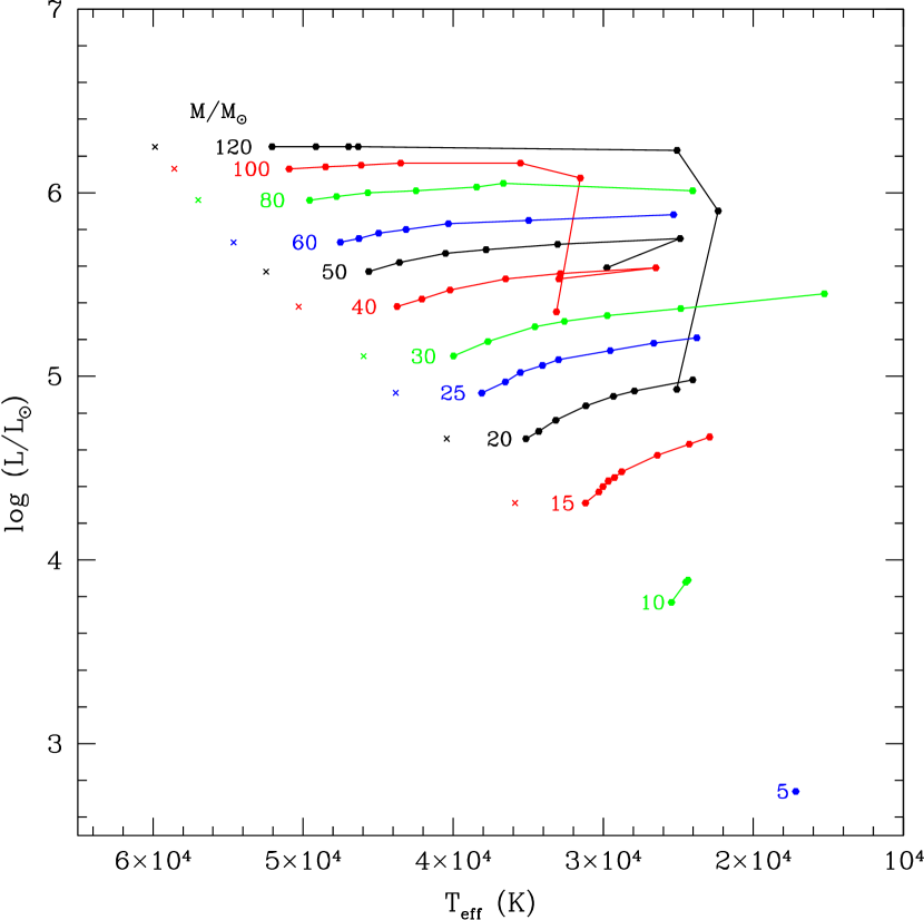
Figure 1.— Grid of WM-basic models. Models were computed for all five metallicities at each point marked in the Hertzsprung-Russell diagram. The grid points (filled circles) were chosen to lie on the solar metallicity evolutionary tracks of Meynet et al. (1994). The labels indicate the zero age masses considered while the lines show the tracks along which each star evolves. On the main sequence, stars of lower metallicity than solar are hotter; we therefore considered additional points at higher temperatures (crosses) to sample this part of the Hertzsprung-Russell diagram. The other stellar parameters used when running the WM-basic models are summarised in Table 1.

2.1.2 Computation of the Grid of Models

WM-basic is distributed by A.W.A. Pauldrach as freeware software on the world wide web and can be run on an IBM-compatible personal computer (PC) with a Microsoft Windows operating system, at least 350 MHz CPU, 64 MB RAM and 200 MB free disk space. For the purposes of this work, it was installed on a 2 GHz Pentium PC in Cambridge and on a 1 GHz Athlon PC in Hawaii, both with 512 MB RAM. Despite the sophistication of the code, the operation of WM-basic is straightforward: the user specifies the stellar parameters of the star to be modelled and the program outputs the corresponding synthetic spectrum. We computed theoretical UV spectra for 87 grid points in the Hertzsprung-Russell (H-R) diagram at each of the five metallicities selected, with an individual model taking between 35 and 80 minutes to run. As we required a high spectral resolution, for improved accuracy, we requested output resolutions of 0.6 Å and 0.25 Å in the wavelength ranges 900–1150 Å and 1150–2124 Å respectively. In the remainder of this section we discuss the selection of the grid points, which are summarised in Table 1 and Figure 1, and the other input parameters used by WM-basic.

As the purpose of our grid of models was to create libraries of theoretical spectra from which Starburst99 could then synthesise the integrated UV spectra of star-forming regions, we first assessed which stars make a significant contribution to the total UV light. This is not immediately obvious because while hotter and more luminous stars produce prodigious amounts of UV flux they are much rarer and shorter-lived than lower mass stars. Simulations using Starburst99 with its empirical libraries show that $\sim 90$% of the UV light at 1450 Å and 1800 Å is generated by stars with zero age main sequence mass greater than 5 $M_{\odot}$. For this reason, we restricted our grid to stars evolving from ones with masses of at least this value.

To run realistic spectral synthesis models one must sample this upper part of the H-R diagram with sufficient grid points. As Starburst99 employs the evolutionary tracks of Meynet et al. (1994) to evolve the stellar population with time, we used these tracks as a guide for which grid points to select. We chose points corresponding to both zero age and evolved stars with initial masses of 120, 100, 80, 60, 50, 40, 30, 25, 20, 15, 10 and 5  $M_{\odot}$, as illustrated in Figure 1. The evolutionary tracks were used to specify the full set of stellar parameters at each grid point, namely luminosity $L$, effective temperature $T_{\rm eff}$ and photospheric radius $R$. We list these values in Table 1.

It is also necessary to specify the stellar wind properties. For simplicity we first discuss stars of solar metallicity. The terminal velocity $v_{\infty}$ of the wind of each star was determined from the empirical scaling formula of Kudritzki & Puls (2000) which relates $v_{\infty}$ to the effective temperature and photospheric escape velocity as follows:

$$v_{\infty}=C(T_{\rm eff})\,v_{\rm esc},\quad{\rm where}$$ (1)

$$C(T_{\rm eff})=2.65,\quad T_{\rm eff}\geq 21,000\,{\rm K}$$

$$C(T_{\rm eff})=1.4,\quad 10,000{\rm K}<T_{\rm eff}<21,000\,{\rm K}$$

$$C(T_{\rm eff})=1.0,\quad T_{\rm eff}\leq 10,000\,{\rm K}.$$

Note that the photospheric escape velocity is defined as

$$v_{\rm esc}=[2gR(1-\Gamma)]^{0.5}$$ (2)

where $g$ is the photospheric gravity, $R$ is the photospheric radius and $\Gamma$ is the ratio of radiative Thomson to gravitational acceleration. This last parameter takes into account the effect of Thomson scattering in weakening the effect of the gravitational potential.

We also had to estimate the mass loss rate $\dot{M}$ from each star in the grid. One of the predictions of radiation-driven wind theory [see Kudritzki (1998) for details] is that a wind momentum–luminosity relation exists such that

$$\log D_{\rm mom}=\log D_{\rm 0}+x\log(L/L_{\odot}),$$ (3)

for

$$D_{\rm mom}=\dot{M}v_{\infty}\,(R_{*}/R_{\odot})^{0.5},$$

where the coefficients $D_{0}$ and $x$ vary with spectral type and (for O stars) with luminosity class. By using the empirical calibrations by Kudritzki & Puls (2000) and the revisions by Markova et al. (2004), we determined the wind momenta and hence mass-loss rates at most grid points. Note, however, that the wind momentum-luminosity relationship of eq. (3), which seems to hold for supergiants and O-type giants, apparently breaks down in O-type dwarfs with luminosities $\log(L/L_{\odot})<5.2$ . For these stars we adopted the relation $\log D_{\rm mom}=12+3\times\log(L/L_{\odot})$ to account for their much weaker winds. The same formula was applied to B-type giants and dwarfs with luminosities $\log(L/L_{\odot})>4.0$ . For lower luminosities a very low value $\log D_{\rm mom}=12$ was adopted to simulate a very weak, unobservable, stellar wind. Values of $\dot{M}$ and $v_{\infty}$ for solar metallicity are listed in the last two columns of Table 1.

Given that stellar winds are believed to be driven by the transfer of photon momentum due to the absorption and scattering of radiation by metal lines, it is expected that the wind properties will be sensitive to the metallicity. To test this assertion observationally, the properties of Galactic hot stars and those in the metal-poor Large and Small Magellanic Clouds have been compared (Puls et al., 1996). While there is clear evidence for smaller terminal velocities in SMC stars (Walborn et al., 1995), further data are required to quantify the dependence of the mass-loss rate on metallicity. Nevertheless, there is an obvious trend for smaller wind momenta in lower metallicity O stars, and investigations are now underway to see whether this is also the case for B and A supergiants. In our models we adopted the best theoretical estimates for the scaling of $v_{\infty}$ and $\dot{M}$ with metallicity, as given by Leitherer et al. (1992), Vink et al. (2001), and Kudritzki (2002, 2003):

$$v_{\infty}=v_{\infty,\,\odot}\,{\left({Z\over Z_{\odot}}\right)^{0.13}}\quad{\rm and}$$ (4)

$$\dot{M}=\dot{M}_{\odot}\,{\left({Z\over Z_{\odot}}\right)^{0.69}}.$$ (5)

Note that the hydrodynamic structure of the WM-basic models is calculated by accounting for a radiative line force in the equation of motion, parameterized by a ‘line force multiplier’. In order to calculate models with pre-specified values of the mass-loss rate and terminal velocity, it is necessary to estimate values of this parameter. To this end, we used the analytical approach by Kudritzki et al. (1989) in an iterative algorithm to provide the WM-basic code with force multipliers that yield the appropriate values of $v_{\infty}$ and $\dot{M}$ as the result of the solution to the equation of motion.

When running the grid at the five metallicities (2, 1, 0.4, 0.2 and 0.05 $Z_{\odot}$), we had the choice of using either (i) WM-basic’s solar reference abundances scaled by a constant factor or (ii) our own choice of individual element abundances. We first consider the case of modelling star-forming regions within our Galaxy of ‘solar’ metallicity. Two possible sets of element abundances are the solar scale and the Orion nebula scale; we compare them in Table 2.1.2. The differences between the two, particularly in some of the element ratios [e.g. (N/O), (Mg/O) and (Si/O)] are still a source of concern; presumably they reflect unresolved systematic errors in either, or both, sets of measurements. In the present work, we adopted the Orion nebula values for elements included in the compilation by Esteban et al. (1998); column (3) in Table 2.1.2 lists the corresponding correction factors we applied to the default solar scale provided by WM-basic. For elements not included in the compilation by Esteban et al. (1998) we used the default solar scale in WM-basic.

Table 2Orion Abundance Scale

X	12+log(X/H)Orion	Correction	12+log(X/H)⊙	Ref	[X/H]Orion
C	8.49	$-0.029$	8.44	1	$+$0.05
N	7.78	$-0.139$	7.93	2	$-$0.15
O	8.72	$-0.112$	8.74	2	$-$0.02
Ne	7.89	$-0.189$	8.00	2	$-$0.11
Mg	7.43	$-0.150$	7.58	3	$-$0.15
Si	7.36	$-0.184$	7.56	3	$-$0.20
S	7.17	$-0.152$	7.20	3	$-$0.03
Cl	5.33	$-0.175$	5.28	3	$+$0.05
Ar	6.49	$+0.093$	6.40	3	$+$0.09
Fe	7.48	$-0.025$	7.50	3	$-$0.02

References. — (1) Allende Prieto et al. (2002) — note that we adopt the C/O ratio from this source and apply it to our solar oxygen abundance; (2) Holweger (2001); (3) Grevesse & Sauval (1998).

Of course there is no reason a priori why the mix of different elements should be the same as in the Orion nebula (or the Sun). Element ratios can (and do) vary as a function of metallicity, reflecting the past history of star formation of a galaxy. Departures from solar ratios are plausible in high redshift star-forming galaxies, given that these objects generally support much higher star formation rates than our Galaxy did at any time in its past. Under these circumstances, elements synthesized by long-lived stars, primarily iron and other Fe-peak elements, may well be underabundant relative to the products of massive stars (oxygen and other $\alpha$-capture elements), as found by Pettini et al. (2002) in MS1512–cB58. While one of the advantages of our fully theoretical approach to synthesizing the UV spectra of star-forming galaxies is that we could in principle choose any mix of elements, for this first attempt we decided to simply scale the Orion nebula abundance pattern to different metallicities, keeping the relative element ratios fixed at their values in the $Z=1Z_{\odot}$ model listed in Table 2.1.2. If the results of the work presented here are sufficiently promising, it will be possible in future to generate models with different abundance ratios to, for example, determine the level of $\alpha$-element enhancement in the galaxies under study.

2.2. Integration of the Spectral Libraries into Starburst99

Ours is the latest in a series of developments and improvements to expand the capability of the spectral synthesis code Starburst99 since it was first released in September 1998. The original version (see Leitherer et al., 1999) did allow some parameters to be calculated at five metallicities (2, 1, 0.4, 0.2 and 0.05 $Z_{\odot}$) thanks to the inclusion of evolutionary tracks and model atmospheres at these metallicities. However, it was only possible to synthesize the emergent ultraviolet spectrum of a star-forming region of solar metallicity because empirical stellar libraries were available only for Milky Way O-type stars. The inclusion of spectra of Galactic B stars in October 1999 (de Mello et al., 2000) allowed the useful spectral range of the synthesized spectra to be extended to 1850 Å where these cooler stars make a significant contribution to the integrated light. The next major development to the code was the introduction in December 2000 of a library of O-type spectra assembled from HST STIS observations of stars in the Large and Small Magellanic Clouds (Leitherer et al., 2001), giving the user the option to synthesize the UV spectrum of a population with a ‘hybrid’ metallicity of about 1/4 solar, albeit over the restricted wavelength range 1250–1600 Å. Most recently, Smith et al. (2002) created a grid of 230 expanding non-LTE line-blanketed model atmospheres, at 2, 1, 0.4, 0.2 and 0.05 $Z_{\odot}$, and incorporated them into Starburst99 for the purpose of calculating realistic ionizing fluxes from young stellar populations.

Smith et al. (2002) utilized two sets of model atmospheres: the WM-basic code by Pauldrach et al. (2001) for O stars and the CMFGEN code by Hillier & Miller (1998) and Hillier & Miller (1999) for Wolf-Rayet stars. Thus, their O-star models were calculated with the same code used in the present study. Since Smith et al. (2002) focused on the emergent ionizing continuum below 912 Å and not on the line spectrum at longer wavelengths, the spectral resolution of their models is not sufficient for the absorption line studies that are the subject of this paper. However, the continuous spectra predicted by Smith et al. (2002) and by us are identical—unless Wolf-Rayet stars were important contributors to the continuum from the integrated stellar population, which is usually not the case.

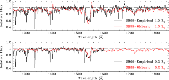
Figure 2.— Comparison of two Starburst99 + WM-basic spectra (red) with ‘conventional’ Starburst99 output spectra generated with empirical libraries of Galactic and Magellanic Clouds OB stars (black). The models shown are for continuous star formation (sampled at an age of 100 Myr when the UV spectral features have fully stabilized) with a Salpeter slope of the IMF between 1 and 100 $M_{\odot}$ and metallicities as indicated. The integrated spectra synthesized with empirical stellar libraries include narrow interstellar absorption lines which are not present in the fully theoretical spectra. The libraries of Magellanic Cloud stars used by Starburst99 only extend to 1600 Å; this accounts for the reduced range of the ‘SB99-Empirical’ spectrum in the lower panel.

For the present work, we built a non-public version of Starburst99 in which the empirical UV library of IUE and HST spectra was replaced by the grid of theoretical spectra generated with WM-basic as described in §2.1. Most of the implementation followed the same steps as the standard version of Starburst99, but with two significant differences, as we now explain.

First, the theoretical spectra are not characterized by spectral types but by their effective temperatures and gravities. Therefore, we can immediately link them to the positions in the H-R diagram predicted by the stellar evolutionary tracks. This is a major advantage over empirical libraries because it avoids the intermediate step of having to adopt a spectral type vs. effective temperature calibration. Recent theoretical and empirical work (Crowther et al., 2002; Bianchi & Garcia, 2002; Martins et al., 2002) has shown that the effective temperature scale of O stars needs to be revised downward from previous calibrations. Such a revision affects spectral synthesis models based on the empirical libraries but not those generated theoretically.

Second, model atmospheres predict both the idealized line-free continuum, and the apparent continuum which includes line blanketing. Therefore we can link the theoretical spectra to the evolutionary models without having to normalize them first. Empirical UV spectra are always affected by an unknown amount of the interstellar reddening. As a result, they must be rectified prior to adding them to a library. Then, the rectified spectra are recalibrated to flux units by fitting a theoretical low-resolution continuum at each grid point in the H-R diagram. This process introduces additional uncertainties which are avoided when a purely theoretical method is employed.

We performed extensive tests with the synthesized spectra. As discussed below (§2.3), the computed photospheric features agree well with those generated with empirical stellar libraries. In addition, the stellar wind lines of C IV $\lambda\lambda 1548,1550$ and Si IV $\lambda\lambda 1393,1402$ show reasonable agreement. However, we believe that a more detailed study of all wind lines is warranted; since these lines are not utilized in the present analysis, their discussion is deferred to a future paper. Once work on the wind lines is completed, we will release an updated version of the Starburst99 code which includes the new theoretical libraries.

With our new, fully theoretical, code we can now model the spectra of star-forming regions as a function of time, for either an instantaneous burst or a continuous star formation law and with a choice of the initial mass function (IMF) slope and mass range, for metallicities of 2, 1, 0.4, 0.2 or 0.05 $Z_{\odot}$.

2.3. Comparison with the Starburst99 Empirical Libraries

Before using our new code to investigate the effects of metallicity on the integrated stellar spectrum, we performed a ‘sanity check’ by comparing the outputs of two of our Starburst99 + WM-basic models with the corresponding model spectra generated in the conventional manner, that is using empirical libraries of stellar UV spectra. Since the latter are available for two metallicities, corresponding to Galactic and Magellanic Cloud stars respectively, we compared them with the fully theoretical spectra generated with $Z=1$ $Z_{\odot}$ and 0.2 $Z_{\odot}$. The comparison is illustrated in Figure 2 for our ‘standard’ case of a continuous star formation model with a Salpeter IMF between 1 and 100 $M_{\odot}$ (see §3). The spectra generated with the WM-basic libraries were smoothed and normalised according to the procedures described in §3.2.

It is important to realise, when comparing the two sets of spectra, that they differ in their interstellar absorption. The empirical stellar spectra, obtained from observations of real stars, include the most prominent UV interstellar absorption lines which can be strong, particularly along sight-lines to the Large Magellanic Cloud. The WM-basic spectra, on the other hand, do not suffer from this contamination and are purely stellar. When this difference is taken into account, Figure 2 shows that there is a reasonably good agreement between the spectra produced by the empirical and theoretical libraries at both metallicities. Some of the discrepancies, such as those at wavelengths greater than 1700 Å in the solar metallicity models, appear to arise from the continuum normalization rather than from intrinsic differences. Of particular interest for the present work are two blends of photospheric absorption lines, at 1360–1380 Å (which also includes the weak stellar wind line O V $\lambda 1371$) and 1415–1435 Å, which Leitherer et al. (2001) showed to be sensitive to metallicity. Inspection of Figure 2 reveals a fairly good correspondence in these wavelength regions.

3. SYNTHETIC UV SPECTRA AT METALLICITIES $Z=0.05-2Z_{\odot}$

3.1. Computation of the Starburst99 Models

Having confirmed that our new version of Starburst99 produces results that are consistent with those generated by the empirical libraries, we can now turn to its application to the study of high redshift star-forming galaxies. In order to do so, it is necessary first of all to specify the mode of star formation. Starburst99 considers two limiting cases, either an instantaneous (i.e. unresolved in time) burst in which all the stars form at time $t=0$ and the stellar population then evolves passively, or continuous star formation at a constant rate. This distinction is important for our purposes because in the burst scenario the integrated spectrum changes rapidly with time, on timescales of a few Myr, reflecting the short lifetimes of the O and B type stars. In this limit, the emergent spectrum is more sensitive to the age than the metallicity of the stellar population. On the other hand, in the constant star formation limit, a quasi-equilibrium is reached within a few tens of Myr, after which there is little spectral variation with time (e.g. Leitherer et al., 1999, 2001). Clearly, such a situation is much more favourable to the use of stellar features as metallicity indicators.

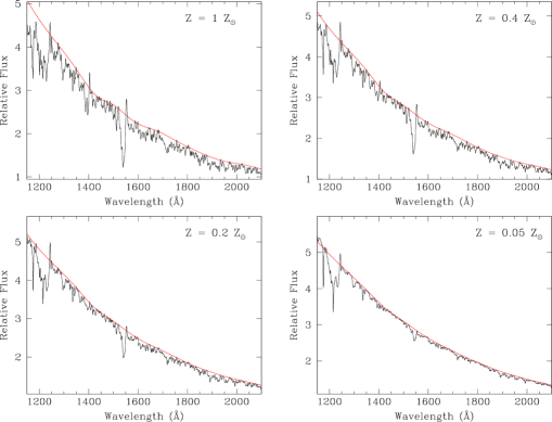
Figure 3.— Examples of the continuum fitting process, showing the spline curves fitted to the ‘pseudo-continuum’ points listed in Table 3. The model spectra shown are for our standard case of continuous star formation (at age 100 Myr) with a Salpeter slope of the IMF between 1 and 100 $M_{\odot}$ and metallicities as indicated.

Table 3Continuum Points

Window	$\lambda_{\rm min}$ (Å)	$\lambda_{\rm max}$ (Å)
01	1274.5	1278.0
02	1348.0	1351.0
03	1439.5	1444.5
04	1485.5	1488.5
05	1586.0	1590.5
06	1678.0	1681.0
07	1754.5	1758.0
08	1800.0	1804.0
09	1875.0	1880.0
10	1968.0	1972.0
11	2018.0	2023.0
12	2072.0	2075.0
13	2110.0	2113.0

Both modes of star formation considered by Starburst99 are idealised approximations to the real progress of star formation in galaxies, which is likely to be a series of bursts. However, when analysing the integrated UV stellar output from a whole galaxy, the continuous star formation mode seems to be the better description, at least for most Lyman break galaxies, as we now explain. If a single burst followed by passive evolution were a valid approximation, we would expect to see large numbers of post-starburst galaxies in which the most massive stars have already died. While still bright in the UV continuum thanks to the longer-lived B stars, such galaxies would lack the nebular emission lines whose strength is determined primarily by the hottest stars present. In other words, while the optical emission lines would fade away after $\sim 10$ Myr, the galaxies would remain UV bright, and still meet the colour criteria tuned to the photometric selection of star-forming galaxies at redshifts $z>1$ (Adelberger et al., 2004), for several tens of Myr. Galaxies with these characteristics seem to be the exception in the surveys by Steidel and collaborators (Pettini et al., 2001; Erb et al., 2003).

In any case, causality arguments alone argue for star formation timescales greater than $30-40$ Myr. This seems to be the characteristic dynamical timescale $\tau_{\rm dyn}=2r_{1/2}/\sigma$ of Lyman break galaxies at $z\simeq 3$, which typically have half-light radii $r_{1/2}\simeq 1-2h^{-1}$ kpc and velocity dispersions $\sigma\simeq 75\pm 25$ km s^-1 (Pettini et al., 2001). Similar values of $\tau_{\rm dyn}$ apply to photometrically selected star-forming galaxies at $z\simeq 1.5-2.5$ [the ‘BX’ and ‘BM’ galaxies surveyed by Steidel et al. (2004) and whose kinematics have been studied by Erb et al. (2003, 2004)]. On the basis of these considerations, we only consider continuous star formation models in the present work.

The second assumption which underlies all stellar population modelling is the shape and the mass limits of the IMF, which is usually approximated by a power law of the form

$$\phi(m)=\frac{{\rm d}n}{{\rm d}m}=Cm^{-\alpha},$$ (6)

(or a combination of such power laws), where $n$ is the number of stars, $m$ is their mass, $C$ is a normalization constant and $\alpha$ is the IMF slope. The slope $\alpha=2.35$ at the upper mass end originally proposed by Salpeter (1955) has stood the test of time (Kennicutt, 1998) and seems to apply to high redshift galaxies too (Pettini et al., 2000; Steidel et al., 2004). Accordingly, in all the modelling presented here we adopted a universal IMF with a Salpeter slope between 1 and 100 $M_{\odot}$ (these being the usual limits used in Starburst99). However, in §4.3.1 we also consider the consequences of adopting different parameters for the IMF.

3.2. Continuum Fitting and Resolution

With the assumption of a continuous star formation mode, with a Salpeter IMF between 1 and 100 $M_{\odot}$ and a constant star formation rate, we used our new version of Starburst99 to compute synthetic spectra, at time intervals of 5 Myr from 5 to 150 Myr, for each of the five metallicities considered. Before analysing these spectra, however, it is necessary to perform a couple of processing steps, as we now explain.

In order to measure any spectral features (whether wind, photospheric, or interstellar lines) it is necessary to first normalize the spectra. This process removes the shape of the underlying continuum by fitting an appropriate function to regions deemed to be free of emission/absorption features and then dividing the spectrum by this function. Second, a comparison between observed and synthesized spectra is best carried out at comparable spectral resolution so that, in general, it is necessary to smooth one spectrum to match the resolution of the other. The important point to be aware of is that continuum fitting and spectral resolution are intimately related. This is because in reality there are very few, if any, wavelength intervals in the UV spectrum of a young stellar population that are truly free of photospheric absorption lines. Thus, smoothing the spectrum invariably results in the depression of even relatively line-free regions and produces an apparent ‘pseudo-continuum’ which is lower than the real continuum level, now no longer discernible.

The primary motivation of this work is to generate a set of fully theoretical spectra which can be compared with those of star-forming galaxies at high redshifts. The largest samples of such galaxies are from the spectroscopic surveys by Steidel and collaborators (Steidel et al., 2003, 2004) conducted with the Low Resolution Imaging Spectrograph (LRIS) on the Keck telescopes. The resolution of this data set, FWHM $\simeq 2.5$ Å in the rest frame, or $\simeq 500$ km s^-1 at 1500 Å, is the major source of line broadening, and dominates over the broadening from internal stellar processes, stellar rotation, and the velocity dispersion of the stars within a galaxy. We therefore simply convolved the synthetic spectra generated by Starburst99 + WM-basic with a Gaussian of FWHM $=2.5$ Å. In order to define the continuum level, we used both our model spectra and actual spectra of Lyman break galaxies to select ‘pseudo-continuum’ points which are listed in Table 3. For each model spectrum, we fitted a spline curve through the mean flux in each of these narrow windows and divided by this fit to produce a normalized spectrum. Figure 3 shows some examples of the spline curves fitted to the models.

Figure 4.— Fully synthetic UV spectra of star-forming regions of metallicities 2–0.05 $Z_{\odot}$. All the models shown are for our standard case of continuous star formation (at age 100 Myr) with a Salpeter slope of the IMF between 1 and 100 $M_{\odot}$. Each spectrum has been convolved with a Gaussian of FWHM $=2.5$ Å and divided by a spline fit to pseudo-continuum points (see Figure 3).

3.3. The Sensitivity of the Stellar Spectrum to Metallicity

Figure 4 presents the smoothed and normalised spectra of the 2, 1, 0.4, 0.2 and 0.05 $Z_{\odot}$ models, 100 Myr after the onset of star formation (by this time the stellar features in the composite UV spectrum have fully stabilised and show no residual time variation). Examination of the figure shows that the spectral appearance is strongly altered by the presence of metals. The most obvious change, as the metallicity decreases, is in the declining strengths of both the absorption and emission components of the stellar wind lines, especially C IV $\lambda\lambda 1548,1550$. Such a marked dependence on metallicity has recently been reported in all the strongest stellar wind lines by Keel et al. (2004) in their study of star-forming regions in nearby galaxies at far-UV wavelengths with the Far-Ultraviolet Spectroscopic Explorer. While it may be tempting to calibrate these features in terms of metallicity, unfortunately (for the present purposes) C IV $\lambda\lambda 1548,1550$ is normally blended with strong interstellar absorption in the spectra of high redshift galaxies (see, for example, Fig. 4 of Pettini et al., 2003). Furthermore, the strengths and profiles of these lines respond not only to metallicity, but also to the slope and upper mass cutoff of the IMF (§4.3.1) and to time dependent dust obscuration (Leitherer et al., 2002). Although there have been attempts to interpret the C IV (and Si IV $\lambda\lambda 1394,1403$) lines in terms of metallicity (e.g. Mehlert et al., 2002), a proper treatment requires careful deblending of the different components (photospheric, wind, and interstellar) which contribute to these composite spectral features. These complicating factors are much less important for the numerous blends of photospheric absorption lines which make up most of the UV spectrum of star-forming regions and which can also be seen from Figure 4 to scale with metallicity.

Following the inclusion of the low metallicity library of empirical stellar spectra into Starburst99, Leitherer et al. (2001) investigated the influence of metallicity upon the spectral appearance of a star-forming region. They drew attention to two blends of lines near 1370 Å and 1425 Å (which they attributed to O V $\lambda 1371$ and Fe V $\lambda\lambda 1360-1380$, and to Si III $\lambda 1417$, C III $\lambda 1427$, and Fe V $\lambda 1430$ respectively) and showed that the equivalent widths of these blends decrease by factors of 2–4 as the metallicity of the stellar population drops from solar to $\sim 1/4$ solar.

We can verify and extend these results with our Starburst99 + WM-basic models. Figures 5 and 6 show the equivalent widths we measure for the ‘1370’ and the ‘1425’ line indices [integrated, as prescribed by Leitherer et al. (2001), over the wavelength ranges 1360–1380 Å and 1415–1435 Å respectively] for different metallicities and ages. These measurements confirm that the lines indices increase monotonically with metallicity over the range $Z=0.05-2Z_{\odot}$ considered here. Equally important is the fact that the indices are stable after $\sim 50$ Myr from the onset of star formation, at which point a quasi-equilibrium is reached with approximately constant relative numbers of each type of star, even though individual stars continuously form and die. Dependence on metallicity and stability with time are both necessary conditions to avoid a degeneracy between age and metallicity which would compromise the usefulness of a line index.

Although our model spectra support the initial suggestion by Leitherer et al. (2001) that the 1370 and 1425 indices may be useful metallicity indicators, these two spectral features are far from ideal for this purpose. First, they are weak, with equivalent widths of only $\lesssim 1.5$ Å at $Z\simeq Z_{\odot}$; therefore their use as metallicity diagnostics requires data of high S/N. A second complication is the fact that these lines are blends of transitions from more than one element and therefore only give some (poorly defined) ‘average’ metallicity. It would not be possible, for example, to use them to investigate departures of different elements from their solar ratios. Finally, their far-UV wavelengths make them difficult to measure from the ground at redshifts lower than $z\sim 1.7$, thereby excluding the large numbers of star-forming galaxies now being discovered at these intermediate redshifts (Steidel et al., 2004; Abraham et al., 2004).

3.4. The Region 1935–2020 Å

Aware of these restrictions, we considered other UV stellar features which do not suffer from the same problems. The most suitable candidate we have found is in the range $\sim$1900–2050 Å. The broad blend of lines in this region was identified thirty years ago with the S2/68 Ultraviolet Sky-Survey Telescope on board the TD1 satellite which provided one of the first views of the sky at ultraviolet wavelengths. From spectrophotometric measurements of early-type stars at a resolution of 35 Å, Thompson et al. (1974) reported the presence of a broad absorption region between 1900 Å and 1940 Å, which they attributed to line blocking by numerous photospheric Fe III transitions (Elst, 1967). A more extensive study by Swings et al. (1976) confirmed that many of the absorption features between 1800 Å and 2200 Å are indeed Fe III transitions. These authors also showed that the strength of the absorption is greater in B-stars of earlier types and higher luminosity classes. Nandy et al. (1981) observed a similar trend for B stars in the Large Magellanic Cloud and noted that the absorption is much weaker in O stars. In a conference proceedings, Morgan et al. (1986) addressed the question of whether the Fe III feature is sensitive to metallicity by studying stars in the metal-poor Small Magellanic Cloud. Their results showed that, on average, the B star absorption is weaker at lower metallicities.

In a study of the ultraviolet properties of nearby starbursts, Heckman et al. (1998) used IUE spectra of $\sim 20$ galaxies to create composite spectra with mean metallicities of $\sim 0.16Z_{\odot}$ and $\sim 1.1Z_{\odot}$. Their work showed that not only is the Fe III absorption clearly visible in the spectra of starburst galaxies but also confirmed that this feature is indeed stronger in higher metallicity environments. In addition to these encouraging preliminary indications, the absorption at $\sim 1900-2050$ Å overcomes many of the difficulties discussed above for the 1370 and 1425 indices. It is broader and stronger, it should be mainly sensitive to the iron abundance, and is accessible from the ground for galaxies down to $z\sim 1$. It therefore merits a closer look.

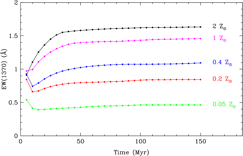
Figure 5.— Variation of the 1370 line index with time and metallicity.

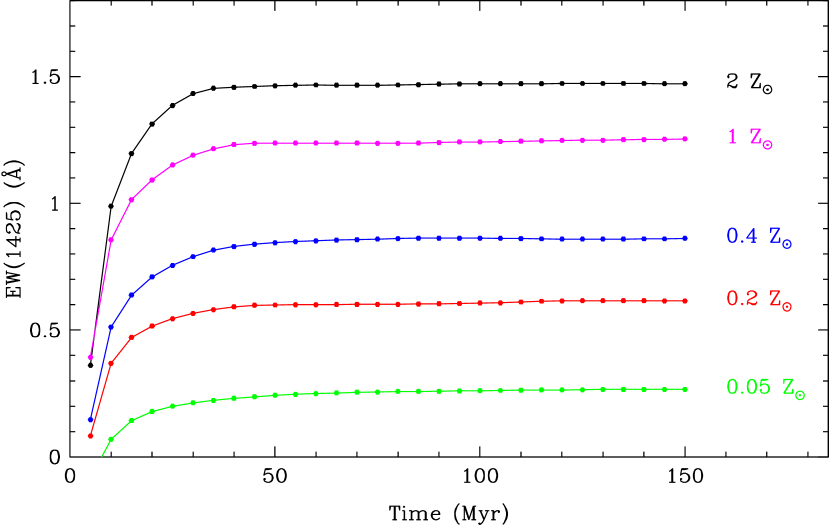
Figure 6.— Variation of the 1425 line index with time and metallicity.

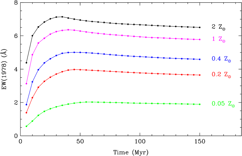
Figure 7.— Variation of the 1978 line index with time and metallicity.

Until now, it has not been possible to model this region of the spectrum, at any metallicity, because the empirical stellar libraries used by Starburst99 do not extend to these mid-UV wavelengths. This is not a problem, however, for WM-basic, and the output from our runs was deliberately chosen to reach beyond 2000 Å (see Figure 4). The spectra shown in Figure 4, which are the first to model the integrated spectrum of a star-forming region at mid-UV wavelengths, indeed confirm that the strength of the Fe III blend increases with increasing metallicity.

To assess its variation with both time and metallicity we have defined a new index, based upon the equivalent width measured between two appropriate wavelengths. In choosing these wavelengths, we took into consideration not only our synthetic models but also the observed spectra of Lyman break galaxies, so as to avoid contamination with other spectral features. Interstellar absorption lines are fortunately not a problem, provided we avoid Al III $\lambda\lambda 1855,1863$ which can be strong (the much weaker Zn II+Mg I blend at $\lambda 2026$ is less of a concern). Potentially more serious is the nebular emission line C III] $\lambda 1909$ which is clearly seen in the composite spectrum of $z\simeq 3$ galaxies generated by Shapley et al. (2003), although its strength can apparently vary substantially between different galaxies.

For these reasons, we decided to restrict the definition of our new metallicity index to the equivalent width measured between 1935 Å and 2020 Å. This defines the ‘1978’ index. In our synthetic spectra, these two integration limits appear to be at wavelengths where the stellar pseudo-continuum is recovered. Figure 7 shows how the index varies with time and metallicity. As was the case for the 1370 and 1425 indices, the 1978 index increases monotonically with metallicity and reaches a steady-state value after $\sim 50$ Myr, thus satisfying both requirements for a useful metallicity indicator. It can also be appreciated, by comparison of Figures 5–7, that at $Z=Z_{\odot}$ EW(1978) is $\sim 4$ times greater than EW(1370) and EW(1425).

4. COMPARISON WITH THE UV SPECTRA OF HIGH REDSHIFT GALAXIES

Table 4Observations of the Rest-Frame UV Spectra of High Redshift Galaxies

Object	$z_{\rm sys}$	${\cal R}$	Instrument	Grating/Grism	Exposure time	$\Delta\lambda_{\rm obs}$	$\Delta\lambda_{\rm rest}$	Resolution	SNR
				(grooves mm-1)	(s)	(Å)	(Å)	(Å)
Q1307–BM1163	1.4110	21.78	LRIS B	0400	05400	3005 –07105	1245 – 2945	2.00	37
MS1512–cB58	2.7276	20.41	ESI	0175	16000	3860 –10500	1040 – 2815	0.37	43
			LRIS R	0900	11400	4300 –06020	1155 – 1615	0.80	75
			LRIS R	1200	03600	5875 –07185	1580 – 1925	0.56	24

To summarize our work so far, we have computed theoretical spectra of OB stars using the stellar wind code WM-basic and integrated them into the spectral synthesis code Starburst99. With this combination, we have generated fully theoretical composite UV spectra of star-forming regions for a range of metallicities, from twice solar to 1/20 solar, under the simplest assumption of continuous star formation with a Salpeter IMF. We have analysed three blends of photospheric stellar lines, at 1370, 1425, and 1978 Å, and found them to be potentially useful metallicity indicators, in that their equivalent widths increase monotonically with metallicity and change little with time after $\sim 50$ Myr (in the idealised approximation of continuous star formation at a constant rate). The 1978 index, developed here for the first time, appears particularly promising in that its equivalent width is larger than those of the other two, it is free of contaminating interstellar lines, and is thought to be due primarily to Fe lines.

Of course, the validity of these photospheric UV indices must be tested against other established metallicity measures before they can be applied with confidence to the study of high redshift galaxies. At present such a comparison is only possible in two cases, the galaxies MS1512–cB58 and Q1307-BM1163. These galaxies are unusually bright, either because they are intrinsically luminous (Q1307-BM1163) or gravitationally lensed (MS1512–cB58), and have been observed over a range of wavelengths at high S/N, allowing measurements of element abundances mostly from interstellar absorption and emission lines. While the preliminary indications from these tests are encouraging, as discussed below, clearly a larger sample of objects suitable for such a cross-check must be assembled for a comprehensive assessment of the method we have developed. We now consider each galaxy in turn; Table 4 gives details of observations of their rest-frame UV spectra with the Keck telescopes. The models shown in the comparisons are all for our standard case of continuous star formation with a Salpeter IMF at age 100 Myr. These models are available in full from Table 5.

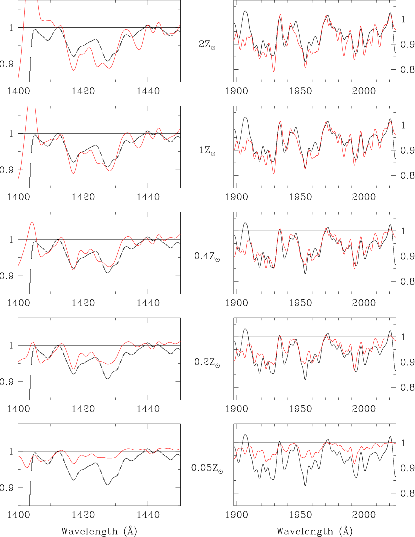
Figure 8.— Comparison of the observed spectrum of the $z=2.7276$ Lyman break galaxy MS1512–cB58 (black) with fully synthetic spectra produced by the Starburst99 + WM-basic combination (red) for five different metallicities, from twice solar to 1/20 of solar. The left-hand set of panels shows the region of the 1425 index (a blend of Si, C, and Fe photospheric lines—see text), while the right-hand set is for the Fe III blend near 1978 Å. Each pair of panels is labelled with the metallicity of the synthetic spectrum shown. The $y$-axis is residual intensity (after normalization by the continuum level).

4.1. MS1512–cB58

Thanks to gravitational lensing by the foreground cluster MS1512+36 at $z=0.373$, MS1512–cB58 (or cB58 for short) is the brightest Lyman break galaxy known and thus one of the most extensively studied. Following its spectroscopic confirmation as a distant galaxy by Yee et al. (1996) (the systemic redshift is $z_{\rm sys}=2.7276$), Pettini et al. (2000) analyzed spectra obtained with the Low Resolution Imaging Spectrometer (LRIS) on the Keck telescope with a view to probing the galaxy’s physical and chemical properties. A more detailed study of the kinematics and chemical abundances of the interstellar gas in cB58 was made possible by high resolution and high S/N ratio observations performed with ESI on Keck (Pettini et al., 2002). Here we compare both the LRIS and ESI data with the synthetic spectra generated by Starburst99 + WM-basic.

Since the observations of cB58 are of unusually high resolution (see Table 4), we first degraded them to the FWHM = 2.5 Å of the synthetic spectra by convolution with Gaussian profiles of the appropriate widths. The spectra were then normalised by division by a spline fit to the continuum points listed in Table 3 [omitting two regions near 1275 Å and 1750 Å where absorption lines from intervening absorption systems, unrelated to cB58, were identified by Pettini et al. (2000)]. We restrict our comparison between observed and synthesized spectra to the wavelength regions of the 1425 and 1978 indices, and neglect the 1370 index which is compromised by lines from two intervening absorption systems, Mg II $\lambda\lambda 2796,2804$ at $z_{\rm abs}=0.8287$ and Si IV $\lambda\lambda 1394,1403$ at $z_{\rm abs}=2.6606$ (Pettini et al., 2000, 2002).

Figure 8 compares portions of the observed spectrum with the corresponding theoretical spectra computed for five metallicities in the 1400–1450 Å (left) and 1898–2025 Å (right) wavelength intervals. We show the LRIS spectrum for the former and the ESI one for the latter (although the ESI spectrum is in general the more useful of the two for such a comparison, it does suffer from poor flux calibration in the 1425 Å region where two echellette orders overlap). The first conclusion to be drawn is that the Starburst99 + WM-basic combination does a remarkably good job at synthesizing ab initio the general character of these spectral regions, attesting to the high degree of sophistication achieved by these codes. Among the five metallicities considered, $Z=1Z_{\odot}$ and $Z=0.4Z_{\odot}$ are those which most closely match the observations in both the 1425 and 1978 regions (giving comparable rms residuals between observed and model spectra).

A metallicity between  $Z_{\odot}$ and $0.4Z_{\odot}$ is in good agreement with other measures. Specifically, the rest-frame optical emission lines analyzed by Teplitz et al. (2000) with the $R_{23}$ method of Pagel et al. (1979) imply an oxygen abundance in the ionized gas of $12+\log{\rm(O/H)}=8.39$, or $\sim 0.5$ of our reference ‘solar’ value $12+\log{\rm(O/H)}=8.72$ in Table 2.1.2 for the Orion nebula. Although less precise, arguments based on the strengths of the P-Cygni profiles of the C IV, Si IV, and N V wind lines also indicate a slightly sub-solar metallicity (Pettini et al., 2000; Leitherer et al., 2001).

By far the most detailed assessment of element abundances in cB58 comes from the study of interstellar absorption lines from cool gas by Pettini et al. (2002). These authors found that among the elements covered in the ESI spectrum of cB58, those which are promptly released into the interstellar medium (Mg, Si, and S) all have abundances of $\sim 0.4$ solar with a scatter of about 0.1 dex, comparable to the measurement error. On the other hand, the Fe-peak elements they observed have a mean metallicity $Z=\left(0.11^{+0.06}_{-0.04}\right)Z_{\odot}$, that is they are less abundant by a further factor of $\sim 4$, which Pettini et al. attribute to a combination of dust depletion and time delay in their release from Type Ia supernovae. Evidently, the iron abundance in the OB stars, as deduced here from the 1978 index, does not agree with the gas-phase abundance of interstellar Fe determined by Pettini et al. (2002), but is close to those of interstellar Mg, Si, O, and S. At face value, (Fe/H)${}_{\rm OB~{}stars}\gtrsim 4\times$ (Fe/H)_gas. This could be an indication that most of the underabundance of interstellar Fe in cB58 is due to dust depletion—an interpretation not favoured by Pettini et al., or that there is an offset in the calibration of the 1978 index with metallicity, or a combination of both. An additional contributing factor may be the unfortunate coincidence that, at the redshift of cB58, the 1935–2020 Å wavelength region is contaminated by telluric absorption; although this was divided out, we could only do so approximately and the process may have left some residual telluric absorption adding to the photospheric Fe III lines.

In summary, we conclude that the analysis of photospheric UV lines from OB stars in cB58, using the methods developed here, yields an estimate of metallicity which agrees with that of the interstellar medium to within a factor of $\sim 2$ (allowing for a moderate degree of dust depletion of the Fe-peak elements).

Table 5Model Spectra for Continuous Star Formation with Salpeter IMF

Wavelength	$Z=0.05Z_{\odot}$	$Z=0.2Z_{\odot}$	$Z=0.4Z_{\odot}$	$Z=1Z_{\odot}$	$Z=2Z_{\odot}$
1150.00	1.025	0.987	0.951	0.890	0.825
1150.18	1.026	0.988	0.951	0.889	0.823
1150.36	1.027	0.989	0.951	0.887	0.821
1150.54	1.028	0.989	0.950	0.886	0.819
1150.72	1.028	0.989	0.949	0.884	0.817
1150.91	1.028	0.988	0.949	0.884	0.817
1151.09	1.028	0.988	0.949	0.884	0.818
1151.27	1.027	0.988	0.949	0.885	0.819
1151.45	1.027	0.988	0.949	0.885	0.820
1151.63	1.026	0.987	0.949	0.886	0.821

Note. — The units of wavelength are Å. The other five columns list values of residual intensity at five different metallicities, as indicated in the column headings. Table 5 is published in its entirety in the electronic version of the Astrophysical Journal. A portion is shown here for guidance regarding its form and content.

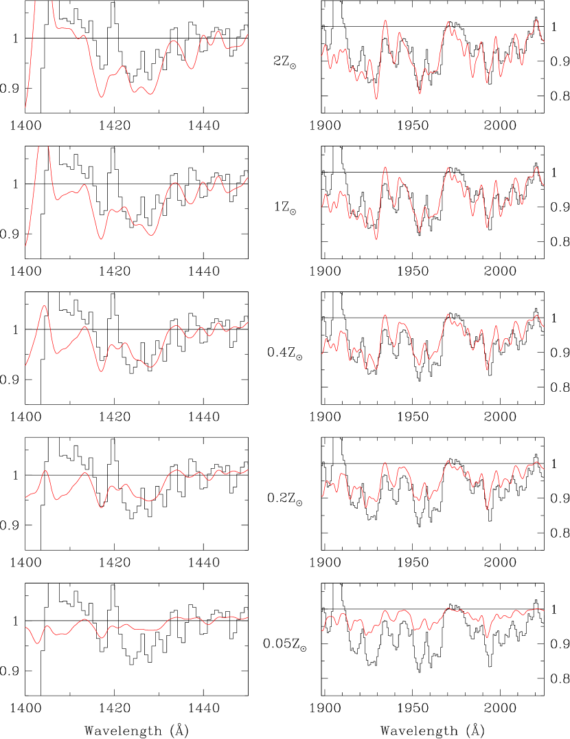
Figure 9.— Comparison of the LRIS-B spectrum of the $z=1.411$ galaxy Q1307–BM1163 from the survey by Steidel et al. (2004) (black) with Starburst99 + WM-basic synthetic spectra for five metallicities (red). Other details are as in Figure 8.

Table 6Summary of Abundance Measurements in MS1512–cB58 and Q1307–BM1163

Galaxy	Redshift	IS Abs. Lines	$R_{23}$	$N2$	1425 index	1978 index
MS1512–cB58	2.7276	$Z=(0.4\pm 0.1)\,Z_{\odot}$	(O/H) = 0.5 (O/H)⊙	$\cdots$	$Z=0.7\,Z_{\odot}$	(Fe/H) = 0.7 (Fe/H)⊙
		(Fe/H) = $\left(0.11^{+0.06}_{-0.04}\right)\times$ (Fe/H)⊙
Q1307–BM1163	1.4110	$\cdots$	$\cdots$	(O/H) $=\left(0.65^{+0.5}_{-0.3}\right)\times$ (O/H)⊙	$\cdots$	(Fe/H) = 1.3 (Fe/H)⊙

4.2. Q1307–BM1163

The combination of high luminosity and relatively low redshift makes the ${\cal R}=21.67$, $z=1.411$ galaxy Q1307–BM1163 one of the brightest in the BM/BX sample of galaxies in the ‘redshift desert’ ($z\simeq 1.4-2.5$) recently assembled by Steidel et al. (2004). These authors reported an oxygen abundance $12+\log{\rm(O/H)}=8.53\pm 0.25$ for the H II gas from the observed [N II] $\lambda 6583$/H$\alpha$ emission line ratio (the $N2$ index of Pettini & Pagel, 2004); this value corresponds to a metallicity $Z=\left(0.65^{+0.5}_{-0.3}\right)Z_{\odot}$ when compared with our reference $12+\log{\rm(O/H)}=8.72$. The profile of the C IV wind line is also consistent with near-solar metallicity (see Fig. 6 of Steidel et al., 2004).

Figure 9 compares the LRIS-B spectrum of Steidel et al. (2004) with our five synthetic spectra, again in the 1400–1450 Å (left) and 1898–2025 Å (right) wavelength intervals. The 1360–1380 Å region is less useful in this case because, at the redshift of Q1307–BM1163, it is close to the blue edge of the LRIS-B spectrum, where the S/N is low. As before, the observations were suitably smoothed to match the resolution of the model spectra (in this case only a moderate amount of smoothing was required, from FWHM $=2$ Å to FWHM $=2.5$ Å) and normalised by reference to the continuum points defined in Table 3. Inspection of Figure 9 indicates that the synthetic spectrum with $Z=0.4Z_{\odot}$ is the closest match (lowest rms difference) to Q1307–BM1163 in the 1415–1435 Å region, while the solar metallicity model reproduces best the Fe III blend near 1978 Å. The latter may be more reliable, given the higher S/N of the data at these wavelengths. However, in either case the conclusion, as for cB58, is that the photospheric UV stellar indices give abundances that agree to within a factor of $\sim 2$ with those deduced from other indicators based on stellar wind lines and nebular emission lines from H II regions.

4.3. The Use of Line Indices

When we assessed the outputs of our code against the spectra of cB58 and Q1307–BM1163 in the preceding sections, we did so by identifying the synthetic spectrum, among five options in metallicity, that gives the smallest rms deviations from the observations. For a more straightforward determination of metallicity, we give here functional forms to the relations between the equivalent widths of the 1425 and 1978 line blends and $\log(Z/Z_{\odot})$. These were deduced by fitting the values measured from our synthetic spectra at the five metallicities for which they were generated, as shown in Figure 10. The values of EW fitted are those from Figures 6 and 7, at time 100 Myr. We find:

$$\log(Z/Z_{\odot})=A\times\mbox{EW}(1425)+B,\quad\mbox{where}$$ (7)

$$A=1.74\quad\mbox{and}\quad B=-1.75 \quad\mbox{EW}(1425)<0.6\mbox{\AA}$$

$$A=1.14\quad\mbox{and}\quad B=-1.39 \quad\mbox{EW}(1425)\geqslant 0.6\mbox{\AA}$$

and

$$\log(Z/Z_{\odot})=C\times\mbox{EW}(1978)+D,\quad\mbox{where}$$ (8)

$$C=0.33\quad\mbox{and}\quad D=-1.94 \quad\mbox{EW}(1978)\leqslant 5.9\mbox{\AA}$$

$$C=0.42\quad\mbox{and}\quad D=-2.50 \quad\mbox{EW}(1978)>5.9\mbox{\AA}.$$

As can be seen from Figure 10, both indices increase linearly, or nearly so, with $\log Z$ over the factor of 40 in $Z$ considered in this work. It is important to realize that the relations given in (7) and (8) above are valid only for spectra of 2.5 Å resolution normalised through the continuum points listed in Table 3. Given the broad, shallow nature of these photospheric blends, their equivalent widths are very sensitive to the continuum normalization which, as explained in §3.2, in turn depends on the spectral resolution of the data.

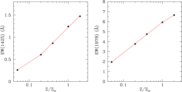
Figure 10.— EW$-Z$ relation for the 1425 and 1978 indices. The dots are the values of equivalent width measured from the synthetic spectra at age 100 Myr, while the lines show the functional fits given by eqs. (7) and (8).

Applying eqs. (7) and (8) to cB58, we find $\log Z=-0.16$ ($Z=0.69Z_{\odot}$) from the measured EW(1425)=1.08 Å, and $\log Z=-0.17$ ($Z=0.68Z_{\odot}$) from EW(1978)=5.37Å. Although in good agreement with each other, these values are somewhat higher than $Z=(0.4\pm 0.1)Z_{\odot}$ determined for the interstellar gas (§4.1). In Q1307–BM1163 we can only measure the 1978 index, because the 1425 blend is affected by a noise spike—see Figure 9. (This is one of the limitations in reducing a whole spectral feature to a single number. While admittedly more objective, this approach is however more vulnerable to noise than the spectral match discussed in §4.1 and §4.2. With the latter it is still possible to recover useful information from ‘clean’ portions of the spectrum). We deduce $\log Z=+0.10$ ($Z=1.3Z_{\odot}$) from the measured EW(1978)=6.2 Å in Q1307–BM1163, which again is somewhat higher than $Z=\left(0.65^{+0.5}_{-0.3}\right)Z_{\odot}$ deduced from the [N II]/H$\alpha$ emission line ratio from H II gas (§4.2).

All the above abundance measurements in cB58 and Q1307–BM1163 are summarised in Table 6. Considering that each of the established methods (interstellar absorption lines, $R_{23}$, and $N2$) give values of metallicity which are only accurate to within a factor of $\sim 2$, the photospheric line indices developed here appear to be a promising alternative. On the basis of this very limited comparison, it would seem that the hot star models tend to slightly underestimate the strengths of the photospheric blends at 1425 Å and 1978 Å at a given metallicity. It would be interesting, in future, to verify if this is indeed the case with a larger set of galaxies where both stellar and H II region abundances have been measured.

Table 7IMF Parameters

Model	Star Formation Mode	IMF slope	$M_{\rm up}~{}(M_{\odot})$
A	Continuous	2.35	100
B	Continuous	3.30	100
C	Continuous	2.35	030

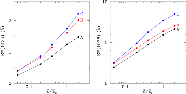
Figure 11.— Dependence of the 1425 and 1978 indices on the IMF parameters. Model A is for our standard case of continuous star formation with a Salpeter IMF at age 100 Myr. Models B and C have comparatively fewer massive stars than model A (see Table 7). The lines here simply join the dots, to guide the eye.

4.3.1 Sensitivity of the Line Indices to the IMF parameters

Finally, we briefly consider the sensitivity of the 1425 and 1978 indices to the IMF parameters. To this end, we generated a new set of synthetic spectra as described in §3, but with different IMF prescriptions, and remeasured values of EW(1425) and EW(1978) at the five metallicities considered in this work. Table 7 gives details of the IMF parameters considered. Model ‘A’ is our standard case of continuous star formation with a Salpeter IMF at age 100 Myr. Model ‘B’ has a steeper power-law slope ($\alpha=3.30$ in eq. 6), and is thus close to the Miller & Scalo (1979) IMF at the high mass end. Model ‘C’ has the standard Salpeter slope but the IMF is truncated at $M_{\rm up}=30\,M_{\odot}$. Thus, both models B and C have comparatively fewer high mass stars than model A.

As can be seen from Figure 11, decreasing the proportion of massive stars consistently increases the equivalent widths of the two blends (at a given metallicity), reflecting the fact that these spectral features are strongest in late O and early B-type stars. However, there are other spectral changes which accompany these IMF alterations. The most obvious one (see Figure 12) is in the character of the C IV $\lambda\lambda 1548,1550$ line which in models B and C no longer exhibits a discernible P-Cygni component, as already noted by Pettini et al. (2000) and Steidel et al. (2004). The empirical observation that Lyman break galaxies normally show such P-Cygni features—as demonstrated by the composite spectrum of Shapley et al. (2003)—argues against significant departures from a Salpeter IMF (at least for masses $M>5\,M_{\odot}$) even at these early epochs.

Figure 12.— Normalised, synthetic UV spectra at solar metallicity for the three sets of IMF parameters listed in Table 7. Model A is for our standard case of continuous star formation with a Salpeter IMF at age 100 Myr. Models B and C have comparatively fewer massive stars than model A.

5. DISCUSSION AND CONCLUSIONS

Rest-frame UV spectra of galaxies at redshifts $z>1$ are now being routinely obtained with large ground-based telescopes. Current samples already include thousands of galaxies with spectroscopic redshifts and their numbers will continue to grow in the years ahead. Encoded in all these spectra is information on the chemical composition of the galaxies which is one of the key physical properties for understanding their previous history and future evolution. Potentially, knowledge of the relative abundances of the chemical elements in these galaxies can tell us about the accumulation of the products of previous stellar generations, the consumption of gas into stars, the pace of star formation activity, the initial mass function, and the importance of inflows and outflows in shaping the chemical evolution of galaxies in the distant past.

In this paper we have taken the first steps towards decoding some of this information. In order to do so, we have found it necessary to synthesize ab initio the spectra of stars at the upper end of the H-R diagram and use them, via a spectral synthesis code, to predict the emergent UV spectrum of a composite stellar population as a function of metallicity. This approach was dictated by the practical difficulties with current facilities to assemble such a library of stellar spectra directly from observations and was made possible by the high degree of sophistication achieved by codes such as WM-basic and Starburst99. A further advantage of a fully theoretical method such as ours is that one has complete control over the wavelength coverage and resolution of the synthesized spectrum, as well as over the metallicity and relative abundances of individual elements.

The results of this initial study are encouraging, in that theoretical and empirical spectra resemble each other closely and in detail—while the models may not be perfect yet, they provide a remarkably good representation of reality.

We have focussed our attention on three blends of photospheric stellar lines, near 1370, 1425, and 1978 Å, and found that they are indeed mostly sensitive to metallicity. In the idealized case of a continuous star formation activity at a constant rate, the equivalent widths of these three features vary little with time after approximately 50 Myr, and increase by factors of $\sim 4-6$ as the metallicity of the stars increases from 1/20 of solar to twice solar. Of the three blends, the one at 1978 Å may be the most useful because: (a) it is the strongest, with an equivalent width EW(1978) $=5.9$ Å at solar metallicity; (b) the wavelength interval 1935–2020 Å over which it is defined is free of strong interstellar lines; (c) its rest-frame wavelength makes it accessible to ground-based spectroscopy over the redshift range $z=1-3$ where recent surveys for high redshift galaxies have been prolific; and (d) it is due primarily to Fe III lines and thus measures the abundance of a single element rather than a combination of several.

We have only been able to test the validity of our method in two cases, by comparing the synthetic spectra we generated with those of two bright high redshift galaxies, MS1512–cB58 at $z=2.7276$ and Q1307–BM1163 at $z=1.411$. We find that in these two cases the metallicities deduced from the photospheric lines agree, to within a factor of $\sim 2$, with those derived from analyses of interstellar absorption and emission lines. More extensive comparisons will allow us to refine the calibrations of our line indices in terms of metallicity.

The principal conclusion of this work is that photospheric UV lines offer a much needed complementary avenue to determining the degree of metal enrichment in high redshift galaxies. The main weaknesses of the method we have developed are: (a) It is based on spectral features that are broad and shallow. Thus, while they can be detected even in spectra of modest resolution, their measurement does require a moderately high signal-to-noise ratio, S/N $\gtrsim 15$ per pixel at $R\simeq 1000$. (b) The equivalent widths of the features in question depend on the mix of spectral types present in a star-forming region. Thus, their strengths would vary with time in isolated bursts of star formation and, to a lesser extent, with the initial mass function. However, to date, neither single bursts nor departures from a universal IMF (at the upper mass end) have been found to be common in high redshift galaxies.

The main strength of the technique is its complementarity to other abundance measures: it is applicable precisely where other techniques fall short. Abundance determinations from interstellar absorption lines require a combination of spectral resolution and S/N that is not achievable with current means for the vast majority of high redshift galaxies. Circumventing this problem by co-adding spectra of many galaxies is fraught with dangers (e.g. Savaglio et al., 2004), since the absorption lines are normally on the flat part of the curve of growth, where their equivalent widths are much more sensitive to the velocity dispersion of the gas than to its column density (and therefore metallicity). Furthermore, most abundant elements are depleted onto dust in the interstellar medium; correcting for unknown and variable amounts of dust depletion is a significant complication which has not yet been fully resolved even in QSO absorption line studies (e.g. Vladilo, 2004).

Emission lines from H II regions, on the other hand, when observed at high redshifts are limited to the strongest lines which sample only a few elements (primarily oxygen). The so-called ‘strong line methods’ give estimates of the oxygen abundance that are only accurate to within a factor of $\sim 2$ [see, for example, the discussion by Pettini & Pagel (2004)], comparable to the accuracy of the photospheric UV line method explored here, at least on the basis of initial tests. Furthermore, there are only a few redshifts intervals at $z>1$ where the nebular lines required for abundance measurements all fall within near-IR windows accessible from the ground, and even then contamination by strong sky emission lines is often a limiting factor to the measurement of reliable line ratios.

Looking ahead, there are thus strong motivations for continuing the work we have begun by: (a) incorporating future improvements in WM-basic into our hybrid code and, (b) most importantly, performing more extensive cross-checks between abundances deduced from nebular emission lines and with our photospheric UV absorption line technique, in cases where both methods are applicable. With a reliable calibration of the latter in hand, we would then have the means to measure stellar abundances in a wholesale manner over a wide range of cosmic epochs.

Table 1Grid of WM-Basic Models

$M$	$\log$ ($L$/$L_{\odot}$)	$T_{\rm eff}$	$\log$ ($g$/cm s-2)	$R$	$\dot{M}$	$v_{\infty}$
($M_{\odot}$)		(K)		($R_{\odot}$)	($M_{\odot}$ yr-1)	( km s-1)
119.98	6.25	59870	4.333	12.39	0.18E-04	4076
119.61	6.25	52061	4.091	16.34	0.17E-04	3545
113.24	6.25	49139	3.965	18.39	0.31E-04	3190
103.40	6.25	46967	3.850	20.06	0.33E-04	2829
string91.79	6.25	46330	3.775	20.59	0.36E-04	2498
string74.11	6.23	25085	2.636	68.66	0.64E-05	1187
string35.76	5.90	22339	2.449	59.17	0.85E-06	0837
string9.15	4.93	25100	3.025	15.43	0.26E-06	1131
string99.63	6.13	58567	4.334	11.27	0.11E-04	3997
string99.75	6.13	50928	4.094	14.87	0.11E-04	3489
string96.50	6.14	48498	3.982	16.65	0.12E-04	3187
string91.23	6.15	46122	3.859	18.64	0.22E-04	2854
string83.46	6.16	43501	3.712	21.13	0.25E-04	2466
string70.95	6.16	35514	3.289	31.71	0.30E-04	1724
string51.76	6.08	31526	3.020	36.90	0.28E-04	1236
string13.17	5.35	33117	3.249	14.30	0.20E-05	1235
string80.13	5.96	57000	4.363	09.79	0.57E-05	4011
string79.86	5.96	49566	4.123	12.87	0.56E-05	3497
string78.64	5.98	47765	4.032	14.19	0.63E-05	3262
string76.50	6.00	45682	3.922	15.89	0.71E-05	2986
string72.72	6.01	42474	3.755	18.75	0.14E-04	2615
string65.85	6.03	38434	3.526	23.24	0.16E-04	2145
string57.50	6.05	36653	3.363	26.20	0.20E-04	1749
string37.09	6.01	24041	2.476	58.40	0.54E-05	0742
string60.07	5.73	54635	4.394	08.17	0.23E-05	3968
string59.94	5.73	47509	4.150	10.82	0.24E-05	3444
string59.43	5.75	46277	4.078	11.70	0.26E-05	3266
string58.68	5.78	44963	3.997	12.76	0.30E-05	3071
string57.54	5.80	43138	3.891	14.28	0.34E-05	2832
string55.65	5.83	40319	3.734	16.82	0.40E-05	2517
string52.28	5.85	34971	3.436	22.98	0.80E-05	2028
string46.34	5.88	25314	2.798	45.11	0.24E-05	1308
string49.97	5.57	52465	4.403	07.37	0.13E-05	3906
string49.96	5.57	45622	4.162	09.73	0.12E-05	3401
string49.23	5.62	43576	4.029	11.27	0.16E-05	3089
string47.81	5.67	40507	3.837	13.85	0.20E-05	2684
string46.55	5.69	37807	3.679	16.39	0.24E-05	2396
string44.20	5.72	33037	3.395	22.14	0.48E-05	1964
string39.75	5.75	24880	2.826	40.41	0.15E-05	1331
string16.89	5.59	29759	2.925	23.51	0.19E-05	0890
string39.94	5.38	50294	4.423	06.45	0.60E-06	3820
string39.97	5.38	43734	4.184	08.49	0.59E-06	3333
string39.50	5.42	42084	4.067	09.66	0.73E-06	3072
string38.78	5.47	40205	3.928	11.23	0.94E-06	2780
string37.45	5.53	36500	3.691	14.49	0.12E-05	2354
string36.28	5.56	32858	3.465	18.51	0.14E-05	2017
string34.37	5.59	26494	3.035	29.55	0.10E-05	1521
string15.70	5.53	32953	3.132	17.87	0.46E-05	1037
string29.95	5.11	45971	4.412	05.65	0.45E-07	3624
string29.99	5.11	39975	4.172	07.46	0.40E-07	3159
string29.33	5.19	37688	3.975	09.25	0.69E-07	2763
string28.47	5.27	34549	3.733	12.04	0.45E-06	2343
string28.02	5.30	32589	3.595	14.01	0.52E-06	2136
string27.43	5.33	29727	3.394	17.46	0.20E-06	1866
string26.55	5.37	24838	3.032	26.07	0.58E-06	1480
string15.62	5.45	15267	1.879	75.41	0.30E-06	0303
string24.97	4.91	43811	4.449	04.95	0.11E-07	3592
string24.99	4.91	38097	4.211	06.50	0.11E-07	3135
string24.61	4.97	36524	4.062	07.66	0.17E-07	2842
string24.35	5.02	35524	3.969	08.49	0.23E-07	2670
string24.02	5.06	34052	3.842	09.75	0.33E-07	2455
string23.81	5.09	32982	3.758	10.70	0.39E-07	2323
string23.25	5.14	29531	3.499	14.25	0.59E-07	1952
string22.85	5.18	26636	3.279	18.19	0.75E-07	1699
string22.41	5.21	23768	3.040	23.73	0.38E-06	1458
string19.96	4.66	40422	4.462	04.36	0.21E-08	3468
string19.99	4.66	35150	4.223	05.74	0.21E-08	3024
string19.85	4.70	34298	4.137	06.32	0.28E-08	2864
string19.61	4.76	33160	4.008	07.28	0.44E-08	2636
string19.28	4.84	31150	3.812	09.04	0.78E-08	2324
string19.06	4.89	29320	3.655	10.78	0.11E-07	2086
string18.92	4.92	27925	3.540	12.26	0.13E-07	1941
string18.54	4.98	24035	3.205	17.85	0.20E-06	1574
string14.98	4.31	35864	4.479	03.70	0.22E-09	3302
string15.00	4.31	31186	4.236	04.90	0.22E-09	2871
string14.91	4.37	30294	4.120	05.58	0.34E-09	2674
string14.88	4.40	30016	4.079	05.85	0.41E-09	2608
string14.84	4.43	29660	4.030	06.18	0.49E-09	2503
string14.80	4.45	29252	3.976	06.56	0.60E-09	2421
string14.75	4.48	28766	3.915	07.03	0.74E-09	2332
string14.60	4.57	26393	3.671	09.27	0.13E-08	2008
string14.50	4.63	24266	3.467	11.68	0.21E-08	1774
string14.43	4.67	22909	3.325	13.72	0.27E-08	1599
string10.00	3.77	25453	4.250	03.94	0.31E-10	2611
string9.99	3.88	24487	4.074	04.82	0.31E-10	2355
string9.99	3.89	24347	4.048	04.97	0.31E-10	2319
string5.00	2.74	17169	4.292	02.65	0.83E-10	1226

Note — The wind parameters  $\dot{M}$ and $v_{\infty}$ refer to the values used for models at solar metallicities. For the remaining metallicities, these parameters were scaled according to eqs. (4) and (5).

References

- Abraham et al. (2004) Abraham, R. G., Glazebrook, K., McCarthy, P. J., Crampton, D., Murowinski, R., Jørgensen, I., Roth, K., Hook, I. M., Savaglio, S., Chen, H., Marzke, R. O., & Carlberg, R. G. 2004, ApJ, 127, 2455
- Adelberger et al. (2004) Adelberger, K. L., Steidel, C. C., Shapley, A. E., Hunt, M. P., Erb, D. K., Reddy, N. A., & Pettini, M. 2004, ApJ, 607, 226
- Allende Prieto et al. (2002) Allende Prieto, C., Lambert, D. L., & Asplund, M. 2002, ApJ, 573, L137
- Bianchi & Garcia (2002) Bianchi, L., & Garcia, M. 2002, ApJ, 581, 610
- Burstein et al. (1984) Burstein, D., Faber, S. M., Gaskell, C. M., & Krumm, N. 1984, ApJ, 287, 586
- Crowther et al. (2002) Crowther, P. A., Hillier, D. J., Evans, C. J., Fullerton, A. W., De Marco, O., & Willis, A. J. 2002, ApJ, 579, 774
- de Mello et al. (2000) de Mello, D. F., Leitherer, C., & Heckman, T. M. 2000, ApJ, 530, 251
- Elst (1967) Elst, E. W. 1967, Bull. Astron. Inst. Netherlands, 19, 90
- Erb et al. (2003) Erb, D. K., Shapley, A. E., Steidel, C. C., Pettini, M., Adelberger, K. L., Hunt, M. P., Moorwood, A. F. M., & Cuby, J. 2003, ApJ, 591, 101
- Erb et al. (2004) Erb, D. K., Steidel, C. C., Shapley, A. E., Pettini, M., & Adelberger, K. L. 2004, ApJ, in press (astro-ph/0404235)
- Esteban et al. (1998) Esteban, C., Peimbert, M., Torres-Peimbert, S., & Escalante, V. 1998, MNRAS, 295, 401
- Faber et al. (1985) Faber, S. M., Friel, E. D., Burstein, D., & Gaskell, C. M. 1985, ApJS, 57, 711
- Feldmeier et al. (1997) Feldmeier, A., Kudritzki, R.-P., Palsa, R., Pauldrach, A. W. A., & Puls, J. 1997, A&A, 320, 899
- Grevesse & Sauval (1998) Grevesse, N., & Sauval, A. J. 1998, Space Science Reviews, 85, 161
- Heckman et al. (1998) Heckman, T. M., Robert, C., Leitherer, C., Garnett, D. R., & van der Rydt, F. 1998, ApJ, 503, 646
- Hillier & Miller (1998) Hillier, D. J., & Miller, D. L. 1998, ApJ, 496, 407
- Hillier & Miller (1999) —. 1999, ApJ, 519, 354
- Holweger (2001) Holweger, H. 2001, in AIP Conf. Proc. 598: Joint SOHO/ACE workshop ”Solar and Galactic Composition”, 23
- Keel et al. (2004) Keel, W. C., Holberg, J. B., & Treuthardt, P. M. 2004, ApJ, in press (astro-ph/0403499)
- Kennicutt (1998) Kennicutt, R. C. 1998, in ASP Conf. Ser. 142: The Stellar Initial Mass Function (38th Herstmonceux Conference), 1
- Kennicutt et al. (2003) Kennicutt, R. C., Bresolin, F., & Garnett, D. R. 2003, ApJ, 591, 801
- Kobulnicky & Koo (2000) Kobulnicky, H. A., & Koo, D. C. 2000, ApJ, 545, 712
- Kudritzki (1998) Kudritzki, R. P. 1998, in Stellar astrophysics for the local group: VIII Canary Islands Winter School of Astrophysics, 149
- Kudritzki (2002) Kudritzki, R. P. 2002, ApJ, 577, 389
- Kudritzki (2003) Kudritzki, R. P. 2003, in IAU Symposium 212, A Massive Star Odyssey: From Main Sequence to Supernova, 325
- Kudritzki et al. (1989) Kudritzki, R. P., Pauldrach, A., Puls, J., & Abbott, D. C. 1989, A&A, 219, 205
- Kudritzki & Puls (2000) Kudritzki, R. P., & Puls, J. 2000, ARA&A, 38, 613
- Leitherer (2003) Leitherer, C. 2003, in A Decade of Hubble Space Telescope Science, 179
- Leitherer et al. (2002) Leitherer, C., Calzetti, D., & Martins, L. P. 2002, ApJ, 574, 114
- Leitherer et al. (2001) Leitherer, C., Leão, J. R. S., Heckman, T. M., Lennon, D. J., Pettini, M., & Robert, C. 2001, ApJ, 550, 724
- Leitherer et al. (1992) Leitherer, C., Robert, C., & Drissen, L. 1992, ApJ, 401, 596
- Leitherer et al. (1999) Leitherer, C., Schaerer, D., Goldader, J. D., Delgado, R. M. G., Robert, C., Kune, D. F., de Mello, D. F., Devost, D., & Heckman, T. M. 1999, ApJS, 123, 3
- Markova et al. (2004) Markova, N., Puls, J., Repolust, T., & Markov, H. 2004, A&A, 413, 693
- Martins et al. (2002) Martins, F., Schaerer, D., & Hillier, D. J. 2002, A&A, 382, 999
- Mehlert et al. (2002) Mehlert, D., Noll, S., Appenzeller, I., Saglia, R. P., Bender, R., Böhm, A., Drory, N., Fricke, K., Gabasch, A., Heidt, J., Hopp, U., Jäger, K., Möllenhoff, C., Seitz, S., Stahl, O., & Ziegler, B. 2002, A&A, 393, 809
- Meynet et al. (1994) Meynet, G., Maeder, A., Schaller, G., Schaerer, D., & Charbonnel, C. 1994, A&AS, 103, 97
- Miller & Scalo (1979) Miller, G. E., & Scalo, J. M. 1979, ApJS, 41, 513
- Morgan et al. (1986) Morgan, D. H., Nandy, K., & Thompson, G. I. 1986, in IAU Symp. 116: Luminous Stars and Associations in Galaxies, 95
- Nandy et al. (1981) Nandy, K., Morgan, D. H., Willis, A. J., Wilson, R., & Gondhalekar, P. M. 1981, MNRAS, 196, 955
- Pagel et al. (1979) Pagel, B. E. J., Edmunds, M. G., Blackwell, D. E., Chun, M. S., & Smith, G. 1979, MNRAS, 189, 95
- Pauldrach et al. (2001) Pauldrach, A. W. A., Hoffmann, T. L., & Lennon, M. 2001, A&A, 375, 161
- Pauldrach et al. (1994) Pauldrach, A. W. A., Kudritzki, R. P., Puls, J., Butler, K., & Hunsinger, J. 1994, A&A, 283, 525
- Pettini & Pagel (2004) Pettini, M., & Pagel, B. E. J. 2004, MNRAS, 348, L59
- Pettini et al. (2002) Pettini, M., Rix, S. A., Steidel, C. C., Adelberger, K. L., Hunt, M. P., & Shapley, A. E. 2002, ApJ, 569, 742
- Pettini et al. (2003) Pettini, M., Rix, S. A., Steidel, C. C., Shapley, A. E., & Adelberger, K. L. 2003, in IAU Symposium 212, 671
- Pettini et al. (2001) Pettini, M., Shapley, A. E., Steidel, C. C., Cuby, J., Dickinson, M., Moorwood, A. F. M., Adelberger, K. L., & Giavalisco, M. 2001, ApJ, 554, 981
- Pettini et al. (2000) Pettini, M., Steidel, C. C., Adelberger, K. L., Dickinson, M., & Giavalisco, M. 2000, ApJ, 528, 96
- Puls et al. (1996) Puls, J., Kudritzki, R.-P., Herrero, A., Pauldrach, A. W. A., Haser, S. M., Lennon, D. J., Gabler, R., Voels, S. A., Vilchez, J. M., Wachter, S., & Feldmeier, A. 1996, A&A, 305, 171
- Puls et al. (1993) Puls, J., Pauldrach, A. W. A., Kudritzki, R.-P., Owocki, S. P., & Najarro, F. 1993, Reviews of Modern Astronomy, 6, 271
- Repolust et al. (2004) Repolust, T., Puls, J., & Herrero, A. 2004, A&A, 415, 349
- Salpeter (1955) Salpeter, E. E. 1955, ApJ, 121, 161
- Santolaya-Rey et al. (1997) Santolaya-Rey, A. E., Puls, J., & Herrero, A. 1997, A&A, 323, 488
- Savaglio et al. (2004) Savaglio, S., Glazebrook, K., Abraham, R. G., Crampton, D., Chen, H.-W., McCarthy, P. J. P., Jørgensen, I., Roth, K. C., Hook, I. M., Marzke, R. O., Murowinski, R. G., & Carlberg, R. G. 2004, ApJ, 602, 51
- Shapley et al. (2004) Shapley, A. E., Erb, D. K., Pettini, M., Steidel, C. C., & Adelberger, K. L. 2004, ApJ, in press (astro-ph/0405187)
- Shapley et al. (2003) Shapley, A. E., Steidel, C. C., Pettini, M., & Adelberger, K. L. 2003, ApJ, 588, 65
- Smith et al. (2002) Smith, L. J., Norris, R. P. F., & Crowther, P. A. 2002, MNRAS, 337, 1309
- Steidel et al. (2003) Steidel, C. C., Adelberger, K. L., Shapley, A. E., Pettini, M., Dickinson, M., & Giavalisco, M. 2003, ApJ, 592, 728
- Steidel et al. (1996) Steidel, C. C., Giavalisco, M., Pettini, M., Dickinson, M., & Adelberger, K. L. 1996, ApJ, 462, L17
- Steidel et al. (2004) Steidel, C. C., Shapley, A. E., Pettini, M., Adelberger, K. L., Erb, D. K., Reddy, N. A., & Hunt, M. P. 2004, ApJ, 604, 534
- Swings et al. (1976) Swings, J. P., Klutz, M., Peytremann, E., & Vreux, J. M. 1976, A&AS, 25, 193
- Taresch et al. (1997) Taresch, G., Kudritzki, R. P., Hurwitz, M., Bowyer, S., Pauldrach, A. W. A., Puls, J., Butler, K., Lennon, D. J., & Haser, S. M. 1997, A&A, 321, 531
- Teplitz et al. (2000) Teplitz, H. I., McLean, I. S., Becklin, E. E., Figer, D. F., Gilbert, A. M., Graham, J. R., Larkin, J. E., Levenson, N. A., & Wilcox, M. K. 2000, ApJ, 533, L65
- Thomas & Maraston (2003) Thomas, D., & Maraston, C. 2003, A&A, 401, 429
- Thomas et al. (2003) Thomas, D., Maraston, C., & Bender, R. 2003, MNRAS, 339, 897
- Thompson et al. (1974) Thompson, G. I., Humphries, C. M., & Nandy, K. 1974, ApJ, 187, L81
- Vink et al. (2001) Vink, J. S., de Koter, A., & Lamers, H. J. G. L. M. 2001, A&A, 369, 574
- Vladilo (2004) Vladilo, G. 2004, A&A, 421, 479
- Walborn et al. (1995) Walborn, N. R., Lennon, D. J., Haser, S. M., Kudritzki, R., & Voels, S. A. 1995, PASP, 107, 104
- Yee et al. (1996) Yee, H. K. C., Ellingson, E., Bechtold, J., Carlberg, R. G., & Cuillandre, J.-C. 1996, AJ, 111, 1783