The Twin–Jet System in NGC 1052:
VLBI-Scrutiny of the Obscuring Torus

NGC 1052 offers the possibility to study the obscuring torus around a supermassive black hole, predicted by the standard model of active galactic nuclei, over a wide range of wavelengths from the radio to the X-ray regime. We present a detailed VLBI study of the parsec-scale structure of the “twin-jet” system in NGC 1052 in both total and polarized intensity and at multiple frequencies. We report the detection of linearly polarized emission from the base of the eastern jet at 5 GHz. While the radio spectrum in this region might be still consistent with synchrotron self absorption, the highly inverted spectrum of the western jet base represents a clear sign of pronounced free-free absorption in a circumnuclear torus. We observe an abrupt change of the brightness temperature gradient at a distance of $\sim 0.2$ pc to $0.3$ pc from the central engine. This might provide an observational signature of the edge of the central torus, where the transition from an external pressure-dominated jet regime to a more or less freely expanding jet takes place. We determine the absorbing column density towards the western jet core to be $\sim 2.2\times 10^{22}$ cm^-2 in good agreement with the values derived from various X-ray observations. This suggests that the nuclear X-ray emission and the jet emission imaged by VLBI originate on the same scales.

1 Introduction

Radio observations of the low-luminosity active galactic nucleus (AGN) NGC 1052 with Very Long Baseline Interferometry (VLBI) at multiple frequencies have revealed the presence of a dense circumnuclear absorber, which obscures the very center of this elliptical galaxy (Kellermann et al. Kel99 (1999); Kameno et al. Kam01 (2001); Vermeulen et al. Ver03 (2003)). Indeed, the standard model of AGNs predicts the existence of an obscuring torus, whose inner surface is expected to be photo-ionized by illumination from the accretion disk. Colder, neutral material forms the outer boundary of the obscuring torus. NGC 1052 provides the possibility to study the physical properties of this obscuring torus complementary in various wavelength regimes and with a variety of observational methods. Particularly, the combination of VLBI and X-ray spectroscopic studies is capable of addressing the same basic questions with complementary methods. Various X-ray observations of NGC 1052 imply a model-dependent column density of $10^{22}$ cm^-2 to $10^{23}$ cm^-2 towards the unresolved nuclear X-ray core (Guainazzi et al. Gua99 (1999); Weaver et al. Wea99 (1999); Kadler et al. Kad04 (2004)) but the angular resolution of X-ray telescopes is not sufficient to measure the accurate position and extent of the absorber. Relativistically broad iron line emission at 6.4 keV is seen in a high-quality X-ray spectrum obtained with the XMM-Newton telescope (Kadler et al. in prep.). Thus, being the first radio-loud AGN with a strong compact radio core that exhibits strong relativistically broadened iron line emission from the inner accretion disk, NGC 1052 provides a unique possibility to study the inter-relation between AGN mass accretion and jet-formation. For future combined VLBI structural and X-ray spectroscopic monitoring observations, it is essential to study in detail the influence of the obscuring torus on the parsec-scale jet structure at radio wavelengths.

NGC 1052 is a moderately strong, variable source in the radio regime, with a luminosity (integrated between 1 GHz and 100 GHz) of $\sim 4.4\cdot 10^{40}$ erg s^-1 (Wrobel Wro84 (1984)) and an unusually bright and compact radio core. Together with the proximity of the source of only 22.6 Mpc this makes NGC 1052 a premier object for VLBI studies, aiming at the ultimate goal of revealing the physical properties of obscuring tori in AGNs. The parsec-scale structure of NGC 1052 shows a twin jet with an emission gap between the brighter (approaching) eastern jet and the western (receding) jet and free-free absorption towards the western jet (Kellermann et al. Kel99 (1999)). Kameno et al. (Kam01 (2001)) suggested the presence of a geometrically thick plasma torus and a geometry of the jet-torus system in which 0.1 pc of the eastern jet and 0.7 pc of the western jet are obscured. The multi-frequency VLBI structure of NGC 1052 has been further studied by Kameno et al. (Kam03 (2003)) and Vermeulen et al. (Ver03 (2003)). The kinematics of both jets at 2 cm have been investigated by Vermeulen et al. (Ver03 (2003)) who report outward motions on both sides of the gap with similar velocities around 0.6 to 0.7 mas yr^-1 corresponding to $\sim 0.25\,c$.

Besides the ionized (free-free absorbing) gas component there are multiple pieces of evidence for atomic and molecular gas in the central region of NGC 1052. H₂O maser emission occurs towards the base of the western jet (Claussen et al. Cla98 (1998)) within the same region that is heavily affected by free-free absorption. Atomic hydrogen is known to exist in NGC 1052 on various scales. Van Gorkom et al. (VanG86 (1986)) imaged the distribution of the Hi gas with a resolution of $1^{\prime\prime}$ using the VLA. They report a structure three times the size of the optical galaxy. Recent VLBI observations resolved Hi absorption features towards the nuclear jet (Vermeulen et al. Ver03 (2003)). Finally, an OH absorption line was also detected by Omar et al. (Oma02 (2002)) and Vermeulen et al. (Ver03 (2003)) but the distribution of the OH gas on parsec-scales has not been investigated so far.

In this work we analyse the multi-frequency structure of NGC 1052 on parsec-scales between 5 GHz and 43 GHz in both total and linearly polarized intensity. In Sect. 2 we describe briefly the observations with the Very Long Baseline Array (VLBA) and the data reduction. Section 3 and Sect. 4 describe the modeling of the source structure with Gaussian components and the process of aligning the images at the four frequencies. The VLBA images of NGC 1052 themselves in total and polarized intensity are presented in Sect. 5. We analyse the frequency dependence of the observed core position in both jets in Sect. 6 and Sect. 7 discusses the spectral analysis. In Sect. 8 we present the brightness temperature distribution along both jets of NGC 1052 and summarize our results in Sect. 9.

2 Observations and data reduction

NGC 1052 was observed on December 28th, 1998 with the VLBA at four frequencies (5 GHz, 8.4 GHz, 22 GHz, and 43 GHz) in dual polarization mode. The data were recorded with a bit rate of 128 Mbps at 2-bit sampling providing a bandwidth of 16 MHz per polarization hand (divided in two blocks of 16 0.5 MHz channels each). The total integration time on NGC 1052 was about one hour at 5 GHz, 8.4 GHz, and 22 GHz each, and about six hours at 43 GHz, to compensate the lower array sensitivity and the lower source flux density. 3C 345 and 4C 28.07 were used as calibrators during the observation. The correlation of the data was done at the Array Operations Center of the VLBA in Socorro, NM, USA, with an averaging time of two seconds. All antennas of the array yielded good data, except the Owens Valley antenna, which did not record data at 8.4 GHz and 22 GHz. The data at 22 GHz and 43 GHz suffered from some snow in the Brewster dish and rain at St. Croix.

The data calibration and imaging were performed applying standard methods using the programs ${\cal A}{\cal I}{\cal P}{\cal S}$ and difmap (Shepherd et al. She97 (1997)). The a-priori data calibration and fringe fitting were performed in ${\cal A}{\cal I}{\cal P}{\cal S}$ using the nominal gain curves measured for each antenna. Instrumental phase offsets and gradients were corrected using the phase-cal signals injected into the data stream during the data recording process. The data were averaged over frequency and exported from ${\cal A}{\cal I}{\cal P}{\cal S}$. Then, the data were read into difmap, edited, phase- and amplitude self-calibrated, and imaged by making use of the clean algorithm. From a careful comparison of the uncalibrated and self-calibrated data, the absolute flux calibration can be (conservatively) estimated to be accurate on a level of $\lesssim 10$ percent.

The data were corrected for the instrumental polarization of the VLBA using the method described by Leppänen et al. (Lep95 (1995)). The absolute values of the electric vector position angles (EVPAs) at all four frequencies were calibrated using the source 3C 345, for which a large data base exists in the literature from which the EVPA in the core and jet regions of this source can be obtained (e.g., Ros et al. Ros00 (2000)).

3 Modeling the source structure

In VLBI imaging the absolute positional information is lost in the phase-calibration process. In the case of simultaneous multi-frequency observations this means that a–priori it is not clear how the images at the different frequencies have to be aligned. The ideal method for overcoming this is to carry out phase-referencing observations, using a compact nearby object and using it to calculate the position of the target source relative to it (e.g., Ros Ros04 (2004)). Our VLBA observations were not phase-referenced, so another way was used to register the four maps. We model fitted the visibility data with two-dimensional Gaussian functions. Those functions, called components, were chosen to be circular to reduce the number of free model parameters and to facilitate the comparison of the models at the different frequencies. The model fitting was performed in difmap using the least-squares method. The errors were determined with the program erfit, a program from the Caltech VLBI data analysis package that calculates the statistical confidence intervals of the fitted model parameters by varying each parameter.

The fits were initially performed independently at the different frequencies to avoid biasing one by another. Once good fits for all four frequencies were obtained, a cross comparison of the resulting maps was made and the fits were modified to get a set of model fits as consistent as possible. Criteria for consistency were:

• regions that show emission at adjacent frequencies should be represented by the same number of components,

• extended components in the outer parts of the jets should become weaker at higher frequencies as they most likely represent optically thin synchrotron emitting regions,

• the inner edges of both jets are expected to shift inwards towards higher frequencies due to opacity effects, i.e., the corresponding model components might have no low frequency counterpart,

• optically-thin features should not show positional changes with frequency.

Table 1 gives the parameters of the final models for the four frequencies. The most distant component in the eastern jet was labeled as A 1, the adjacent inner one as A 2, and so on. The western jet was divided into three parts following the convention introduced above. The model fit component in the innermost part of the western jet were labeled as B 2b, B 2a, B 1 from east to west. Further out, the components C3b, C3a, C2, C1, and D follow.

Table 1: Model fit parameters

Flux Id density Radius^a P.A. FWHM [mJy] [mas] [^∘] [mas] 5 GHz, $$\chi_{\rm red}=1.12 \pm \pm \pm \pm \pm \pm \pm \pm \pm \pm \pm \pm \pm \pm \pm \pm \pm \pm \pm \pm \pm \pm \pm \pm \pm \pm \pm \pm \pm \pm \pm \pm \pm \pm \pm \pm \pm \pm -114.2 \pm \pm \pm \pm -115.74 \pm \pm \pm \pm -119.6 \pm \pm \pm \pm -114.7 \pm \pm \chi_{\rm red}=1.76 \pm \pm \pm \pm \pm \pm \pm \pm \pm \pm \pm \pm \pm \pm \pm \pm \pm \pm \pm \pm \pm \pm \pm \pm \pm \pm \pm \pm \pm \pm \pm \pm \pm \pm \pm \pm \pm \pm \pm \pm \pm \pm \pm \pm \pm \pm -119.8 \pm \pm \pm \pm -119.9 \pm \pm \pm \pm -114.2 \pm \pm \pm \pm -114.9 \pm \pm \pm \pm -119.1 \pm \pm \pm \pm -114.7 \pm \pm \chi_{\rm red}=0.71 \pm \pm \pm \pm \pm \pm \pm \pm \pm \pm \pm \pm \pm \pm \pm \pm \pm \pm \pm \pm \pm \pm \pm \pm \pm \pm \pm \pm \pm \pm \pm \pm \pm \pm -123 \pm \pm \pm \pm -115 \pm \pm \pm \pm -132 \pm \pm \pm \pm -116.4 \pm \pm \pm \pm -116 \pm \pm \chi_{\rm red}=0.83 \pm \pm \pm \pm \pm \pm \pm \pm \pm \pm \pm \pm \pm \pm \pm \pm \pm \pm \pm \pm \pm \pm \pm \pm \pm \pm \pm \pm \pm \pm \pm \pm \pm \pm \pm \pm \pm \pm \pm \pm \pm \pm -119.2 \pm \pm \pm \pm -120.9 \pm \pm \pm \pm -116.5 \pm \pm$$ A1 802 14.560.03 66.50.1 2.140.03 A2 542 12.010.04 63.60.1 1.870.08 A3 602 9.610.05 65.30.3 1.630.04 A4 1507 7.460.05 71.70.2 0.990.02 A5 33837 6.00.2 72.80.1 0.930.25 A6 44748 5.10.1 72.80.2 0.830.19 A7/8 45028 4.00.1 71.00.2 0.690.08 A9 39730 3.10.2 71.10.3 0.200.07 A10 14037 2.30.2 70.90.4 0.460.05 C3 1373 3.840.03 0.1 1.030.06 C2 593 4.750.06 0.3 0.830.09 C1 241 7.190.03 0.4 1.850.10 D 671 11.810.01 0.1 2.240.05 8.4 GHz, A1 381 14.700.03 66.50.1 2.000.03 A2 371 12.040.04 64.00.1 2.340.08 A3 361 9.300.05 65.90.3 1.620.04 A4 834 7.340.05 71.90.2 0.980.02 A5 728 6.40.2 72.70.1 0.590.25 A6 36026 5.50.1 72.80.2 0.810.12 A7 39622 4.40.1 72.30.2 0.740.06 A8 1468 3.80.1 69.70.2 0.280.06 A9 36021 3.20.2 71.30.3 0.340.05 A10 31647 2.70.2 69.20.4 0.310.03 A11 13725 1.90.2 74.30.4 0.340.07 B2a/b 564 0.600.03 0.1 0.360.02 B1 292 1.260.03 0.1 0.310.02 C3 201 3.750.03 0.1 1.060.08 C2 774 4.860.06 0.3 0.900.09 C1 211 7.030.03 0.4 1.680.10 D 481 11.950.01 0.1 2.210.05 22 GHz, A6 1385 5.480.03 72.40.2 0.980.04 A7 1407 4.390.01 72.20.2 0.650.03 A8 995 3.720.01 68.10.2 0.470.03 A9 1396 3.090.01 72.20.2 0.320.02 A10 1445 2.700.01 68.50.2 0.270.01 A11 448 1.980.04 73.00.8 0.290.07 A12 8615 1.530.04 72.10.4 0.260.06 A13 5414 1.200.04 71.10.9 0.220.06 B2b 34114 0.520.02 1 0.210.01 B2a 15114 0.720.05 2 0.290.02 B1 312 1.380.02 1 0.31.7 C3a 504 3.340.02 0.4 0.580.03 C3b 866 4.180.07 1 1.950.16 43 GHz, A6 402 5.360.03 72.80.2 0.920.05 A7 442 4.390.01 72.20.2 0.510.03 A8 392 3.760.01 68.70.1 0.460.03 A9 371 3.1770.003 71.80.1 0.220.01 A10 701 2.7720.004 68.40.1 0.330.01 A11 191 1.950.01 71.60.5 0.320.03 A12 572 1.4990.004 70.20.2 0.220.01 A13 432 1.2210.006 70.80.2 0.120.01 A14 541 1.0170.003 71.90.2 0.080.05 A15 191 0.470.01 612 0.210.03 B2b 2252 0.4670.002 0.3 0.2240.002 B2a 312 0.7790.007 0.6 0.220.01 C3b 272 3.330.05 0.8 0.950.08

• The radius is measured from the center between A15 and B2b (see Section 4.6).

4 Image alignment

Figure 1: The aligned VLBA images of NGC 1052 at 5 GHz, 8.4 GHz, 22 GHz, and 43 GHz. Contours and beam sizes are given in Table 2.

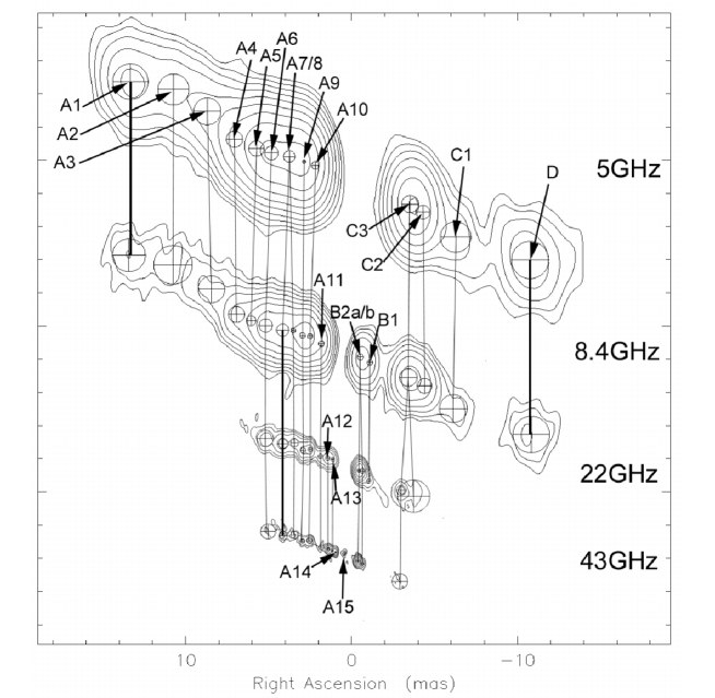
Figure 2: The aligned model-fit maps. The circles represent the full width at half maximum (FWHM) of the circular Gaussians. The vertical and oblique lines join the associated components between different frequencies. The components A 1 and D between 5 GHz and 8.4 GHz and A 7 between 8.4 GHz, 22 GHz and 43 GHz (joined by a thicker trace) were used for the alignment. The lowest contours are 1.9 mJy/beam for the 5 GHz model, 2.6 mJy/beam for the 8.4 GHz model, 5.0 mJy/beam for the 22 GHz model and 3.5 mJy/beam for the 43 GHz model.

The image alignment was performed in two steps. i) The fitted components at the different frequencies were cross–identified and the relative shifts between the models were determined, assuming frequency-independent positions of optically thin features. ii) An origin was determined from which absolute distances could be measured. This method of alignment is not a–priori definite. It is based on the assumption that optically-thin components have frequency-independent positions and that the cross identification of the model components is correct. However, all possible alternative identifications could be ruled out for consistency reasons (by making use of the component flux densities at adjacent frequencies).

We used the two most distant components (A 1 and D) to align the 5 GHz and the 8.4 GHz models by assuming that the mid-point between both components was spatially coincident. Because these two outer components are optically thin and not detectable above 8.4 GHz, the position of component A 7, which is relatively strong at all three frequencies, was used to align the three high-frequency models relative to the origin determined from the alignment of the two low-frequency models. As a natural choice, the most probable position of the true center of jet activity, namely the center between the components A 15 and B 2b, was used as the origin (compare Sect. 6). The component positions in Table 1 are given relative to this reference point.

5 The brightness distribution in total and polarized intensity

5.1 Total intensity imaging

Figure 1 shows the aligned uniformly weighted total intensity images of NGC 1052 at the four frequencies and Fig. 2 shows the images that result from applying Gaussian model-fit components to the measured visibilities. Table 2 gives the image parameters of Fig. 1.

The basic source structure is formed of two oppositely directed jets divided by an emission gap. The source can be divided into four regions: region A makes up the whole (more or less continuous) eastward-directed jet emission; region B is not visible at 5 GHz, but becomes the brightest and most compact feature at high frequencies; regions C and D are bright only at low frequencies and become faint and diffuse at high frequencies. The main source characteristics are summarized in Table 3. A sub-division can be performed based on the Gaussian model fits, found to represent the source structure (see Fig. 2). Region A is sub-divided into the components A 1 to A 15, region B into the components B 1, B 2a, and B 2b, and region C into the components C 1, C 2, and C 3.

Whilst the eastern jet is only slightly curved at distances from the gap larger than 4 mas the counterjet exhibits strong curvature most pronounced at 22 GHz. The jets appear nearly symmetric in the 5 GHz and 8.4 GHz images, becoming asymmetric at higher frequencies. While the emission gap is most prominent at 5 GHz the images at 8.4 GHz, 22 GHz, and 43 GHz reveal jet components occupying this gap region, leaving a smaller but still prominent emission gap. The frequency dependence of the VLBI “core” positions, the points were the eastern and the western jet become optically thin can clearly be seen in Fig. 1. This so-called “core shift” will be analysed in detail in Sect. 6.

Table 2: Total intensity image parameters

• Total flux density recovered in the image

• Corresponds to the A component

• Corresponds to the B component

Table 3: Source characteristics on mas-scales

5.2 Linearly polarized intensity imaging

Figure 3 shows the linearly polarized intensity and its EVPA overlaid on the total intensity image at 5 GHz. A region of linearly polarized emission is visible at the base of the eastern jet. The peak is about 3 mJy per beam and the EVPA is about 70^∘, roughly parallel to the jet. To decide whether the region of linearly polarized emission is resolved, slices along the jet axis of both the total intensity image and the polarization image were produced, using the task slice in ${\cal A}{\cal I}{\cal P}{\cal S}$ (inlayed panel in Fig. 3). In this plot, the polarized emission peaks about 1 mas offset from the total-intensity maximum. A comparison to Fig. 2 ascribes this part of the jet to component A 10, which is optically thick at 5 GHz. The asymmetry of the polarized emission slice suggests the presence of at least two components. The polarized emission is thus slightly resolved and originates in the optically thick part of the eastern jet at 5 GHz.

No linearly polarized emission at a flux density level above 1 mJy could be detected at the other three frequencies Usually, the degree of polarization rises with frequency since beam depolarization reduces the degree of polarization at lower frequencies more strongly than at higher frequencies. Thus, one expects the eastern jet to exhibit polarized emission from the region around component A 10 and A 11 at 8.4 GHz also. Assuming that the polarization has the same (flat) spectrum as the total intensity in this region, it should reach $\sim 3$ mJy per beam at 8.4 GHz (comparable to the polarized flux at 5 GHz). However, this is not observed. At higher frequencies these components become optically thin (compare Sect. 7) and thus fall in total intensity. Were their emission polarized to the same degree as at 5 GHz it would be $<1$ mJy per beam and would thus lie below the detection threshold. The non-detection of linear polarization at the high frequencies in our observations is consistent with the results of Middelberg et al. (Mid04 (2004)) who report unpolarized emission from NGC 1052 at 15 GHz down to a limit of 0.4 %.

Figure 3: 5 GHz image of the polarized emission in NGC 1052 (EVPA superimposed on the total intensity). The inlayed panel shows the total intensity and polarized emission profiles along the slice marked with the dashed line.

6 Identifying the center of activity

The symmetry between the jet and the counterjet constrains the position of the central engine in NGC 1052. The cores of both jets are located at the distances to the central engine, $r_{c}$, where the optical depth $\tau$ has fallen to $\sim 1$. In a conical jet geometry this distance is given by: $r_{c}\sim\nu^{-\frac{1}{k_{r}}}$, (see, e.g., Lobanov Lob98 (1998)) where $k_{r}=((2\alpha-3)b-2n-2)/(5-2\alpha)$, with $\alpha$ being the spectral index and $b$ and $n$ the power indices of the magnetic field and the density of the emitting particles: $B\sim r^{b}$, $N\sim r^{n}$ (Lobanov Lob98 (1998)). Taking logarithms leads to:

$$\log(r_{c})=-\frac{1}{k_{r}}\log(\nu)+const.$$ (1)

Measuring $r_{c}$ at two frequencies allows one to determine $k_{r}$ in the corresponding region of the jet. For a freely expanding jet in equipartition (Blandford & Königl Bla79 (1979)), $k_{r}$=1. The value of $k_{r}$ is larger in regions with steep pressure gradients and may reach 2.5, for moderate values of $m$ and $n$ (Lobanov Lob98 (1998)). If external absorption determines the apparent core position, comparable density gradients of the external medium can alter $k_{r}$ to values above 2.5.

The values of $k_{r}$ deduced depend crucially on the absolute values of $r_{c}$ on the two sides and therefore on the assumed position of the central engine. Four scenarios have been tested with different reference points (see Fig. 4). Table 4 gives the derived values of $k_{r}$ for each scenario. In each case the position of component A 14 has been assumed as the core of the eastern jet, rather than A 15. The latter is comparably weak and, thus, most likely does not represent the true jet core. A 15 might rather represent a bright but heavily self-absorbed new jet component. Formally, however, the $k_{r}$ values for the scenarios 1,2, and 4 between 22 GHz and 43 GHz change to $1.4\pm 0.06$, $0.6\pm 0.03$, and $1.0\pm 0.04$ if A 15 instead of A 14 is used. For scenario 3, A 15 cannot be associated to the eastern jet core (compare Fig. 4).

The area between the model components A 15 and B 2b is the most likely location of the central engine and the center between both components is a natural choice for its exact position (scenario 1). Shifting the reference point eastwards (scenarios 2 and 3) alters the values of $k_{r}$ into unphysically large regimes (requiring density gradients $\propto r^{-10}$ and higher). Assuming the true center of activity to be located more westwards (closer to B 2b, scenario 4), the values of $k_{r}$ derived are still acceptable.

The positions of the bases of both jets at the different frequencies for the first case (scenario 1) are shown in Fig. 5. The eastern jet has rather high values of $k_{r}$ below 22 GHz, although still in agreement with steep pressure gradients in the jet environment. Above 22 GHz $k_{r}$ is 3.9$\pm$0.8, which is a good indicator for free-free absorption affecting the jet opacity. The western jet has values of $k_{r}$ as high as 6.8$\pm$2.7 between 22 GHz and 43 GHz, suggesting a large contribution from free–free absorption.

The results from the core shift analysis support the picture of a free–free absorbing torus covering mainly the inner part of the western jet and also a smaller fraction of the eastern jet. The true center of activity in NGC 1052 can be determined to lie between the model components A 15 and B 2b, with an uncertainty of only $\sim 0.03$ pc.

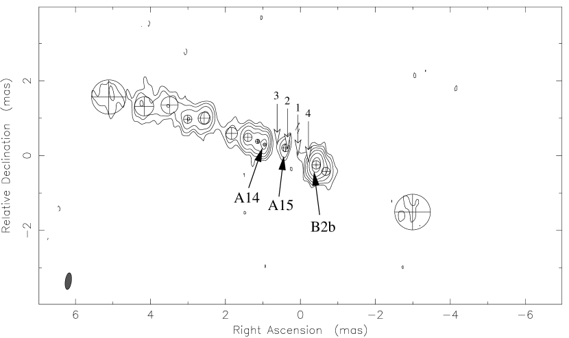
Figure 4: Image with the model fitting results of the 43 GHz data. The innermost jet components are labeled. The putative locations of the central engine are indicated for four different scenarios (see discussion in the text).

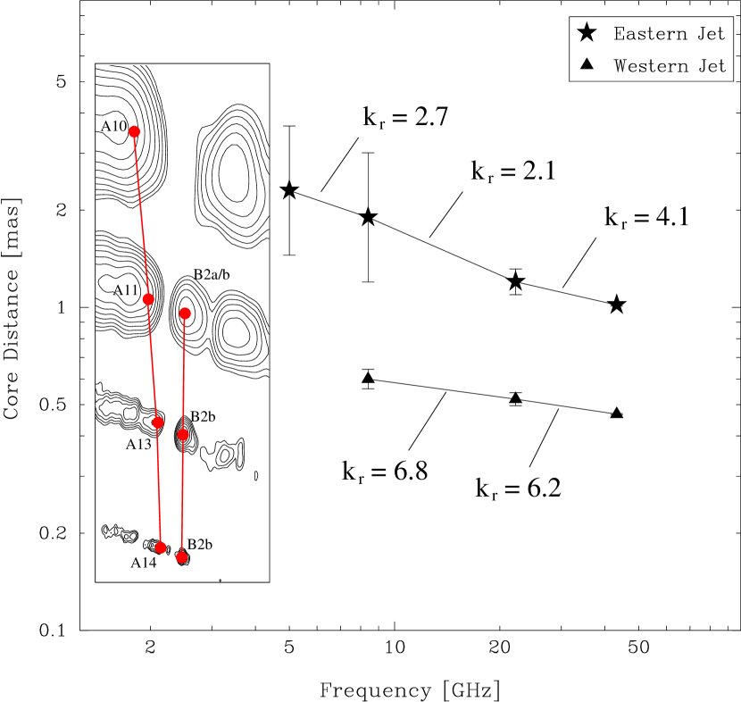
Figure 5: Core positions in the two jets at the different frequencies for scenario 1 (see Fig. 4). Table 4 provides the values of $k_{r}$ for the other two scenarios. The inset panel shows the core locations in the source at the four frequencies.

Table 4: Values of $k_{r}$ for the four different putative centers of activity

7 Spectral analysis

Spectral information can be derived from multi-frequency VLBI data in two ways. The first approach is to use the knowledge of the proper alignment of the total intensity images to derive images of the spectral index between two adjacent frequencies. The second approach is to derive spectra of the model fit components. The approaches are somewhat complementary. The latter gives a handy number of component spectra, which can be analysed in detail, whereas the spectral index imaging gives the full course of the spectral index along the jet axis. Particularly, this yields spectral information at parts of the jet that are not adequately represented by Gaussian model components. The results of both approaches will be presented in this section.

7.1 Spectral index imaging

Spectral index images have been produced using the ${\cal A}{\cal I}{\cal P}{\cal S}$ task comb. For this, the total intensity has been reimaged with appropriate tapering of the $(u,v)$-data to match the resolutions at adjacent frequencies. Information below 1 mJy/beam was discarded in both input images. Table 5 gives the restoring beams and the other relevant parameters of the derived images. The spectral index images are shown in Fig. 6.

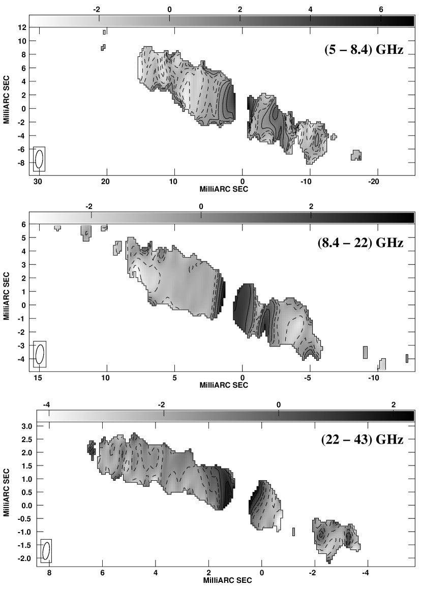
Figure 6: Spectral index images of NGC 1052. The contours and beam parameters are given in Table 5. Note the different scales in the three images and that the images are centered on component B 2.

The main feature in each image of the spectral index is an optically thick inner edge of the innermost part of both jets. Outwards along the jets, the spectral index tends to decrease. The spectral index $\alpha$ exceeds the value of 2.5, the theoretical upper limit for synchrotron self-absorption, on both sides of the gap in the (5–8.4) GHz spectral index image and on the eastern side of the gap also between 8.4 GHz and 22 GHz. High values of $\alpha$ are also reached on the western side of the gap in the (8.4–22) GHz spectral index image and on both sides between 22 GHz and 43 GHz, which however do not exceed the critical value of 2.5. Towards the outer jet regions the spectral index typically falls to values $\lesssim-1$ in the whole frequency range between 5 and 43 GHz. This suggests that the emission from these outer jet regions far from the gap is optically thin above 5 GHz.

Table 5: Spectral index image parameters

$\nu_{1}$	$\nu_{2}$	Common Beam	Cutoff
[GHz]	[GHz]	[mas$\times$mas, ∘]	[mJy/beam]
5	8.4	2.64$\times$1.06, $-$3.81	2
8.4	22	1.42$\times$0.57, $-$5.75	1
22	43	0.66$\times$0.24, $-$7.78	1

7.2 Spectral analysis of the model fit components

The flux densities of the model fit components (see Figure 2) can be used to derive spectra of i) the whole parsec-scale structure, ii) the two jets separately and iii) the model fit components themselves. In Fig. 7, the total spectrum of the parsec-scale structure of NGC 1052 between 5 GHz and 43 GHz is shown, as well as the spectra of both jets separately. All values were obtained by adding up flux densities of model components (A 1 to A 15 for the eastern jet and B 2b to D for the western one).

At the high frequencies both jets show similar spectra with an optically thin decrease of the flux density above 22 GHz. The spectral index in this regime is around $-1$ in both jets, with the eastern jet being significantly stronger than the western one in agreement with the interpretation that the eastern jet approaches the observer whereas the western jet is the counterjet. However, below 22 GHz the spectra of the two jets differs substantially. The eastern jet spectrum remains optically thin above 8.4 GHz and flattens around 5 GHz. The western jet, on the other hand, exhibits a sharp decrease in flux below 22 GHz. Although the spectral index limit of 2.5 is not exceeded, synchrotron self-absorption seems very unlikely to be responsible for the turnover of the spectrum because of two reasons. First, the similarity of the spectra of eastern and western jet at high frequencies suggests similar intrinsic physical properties on both sides so that the self absorption frequency should not differ by a factor of three. Second, the kinematical analysis of Vermeulen et al. (Ver03 (2003)) shows the jet axis to be close to the plane of the sky and the motions to be only weakly relativistic. There is little evidence for strong Doppler boosting. Moreover, such an effect should shift the turnover frequency of the counterjet to lower frequencies, rather than to higher ones. In Sect. 8.3 we will use the moderate velocity differences, on the one hand, and the more pronounced brightness-temperature difference of jet and counterjet, on the other hand, to constrain the orientation of the jet-counterjet system.

Figure 7: Spectrum of the parsec-scale structure of NGC 1052 between 5 GHz and 43 GHz (total and for both jets separately). Errorbars are shown only if they exceed the symbol size.

If the spectrum of the western jet is decomposed into the spectra of the different jet regions B, C and D (see Fig. 1 and Fig. 8) it turns out that the region B, the innermost region on the western side, is responsible for the inversion of the western jet spectrum below 22 GHz.

Figure 8: Spectra of the four jet regions A, B, C and D (see Fig. 1 for the definition of the jet regions). The arrows indicate that component C is partly resolved at 43 GHz and component B is not detected at 5 GHz. Thus, the shown values represent only a lower and upper limit , respectively. Errorbars are shown only if they exceed the symbol size.

Its spectrum between 5 GHz and 8.4 GHz is highly inverted with a spectral index $>4$ since it is not detectable at all at 5 GHz. Such a spectral index cannot be due to synchrotron self absorption but indicates a region of external absorption towards the core of the western, receding jet. The highly inverted spectrum of this component in NGC 1052 and the necessity of an external absorber was first mentioned by Kellermann et al. (Kel99 (1999)) and later confirmed by Kameno et al. (Kam01 (2001)) and Vermeulen et al. (Ver03 (2003)).

It is not clear whether the eastern jet is also affected by external absorption. Kameno et al. (Kam01 (2001)) proposed a geometry in which the obscuring torus, covers 0.7 mas of the western jet and 0.1 mas of the eastern jet. Emission from A 11 is not detected at 5 GHz. Estimating (conservatively) a flux density of 10 mJy at 5 GHz yields a spectral index of $\sim 5$. This would suggest that the innermost part of the eastern jet is also strongly affected by external absorption. However, if the flux densities of the two components A 10 and A 11 are summed at 5 GHz and 8.4 GHz, one obtains a spectral index of 2.3, which is close to that expected for pure synchrotron self-absorption. Consequently, due to the small separations between the inner components in the eastern jet, we cannot finally judge from this approach whether free-free absorption plays an important role. Kameno et al. Kam03 (2003) determined a spectral index of $3.28\pm 0.27$ for the base of the eastern jet between 1.6 GHz and 4.8 GHz and attribute this to free-free absorption in the obscuring torus.

The jet-to-counterjet ratio of NGC 1052 can be determined from the model fitted flux densities of both jets. Figure 9 shows the ratio of the flux densities of the model components on either side of the gap as a function of frequency.

Figure 9: The jet-to-counterjet ratio determined from the flux densities of the model fit components as a function of frequency. Errorbars are shown only if they exceed the symbol size.

At high frequencies the jet-to-counterjet ratio is $\sim 1.5$ and starts rising towards lower frequencies below 22 GHz. At 8.4 GHz the jet is brighter than the counterjet by a factor of $\sim 5$ and at 5 GHz the jet outshines the counterjet even by a factor of $\sim 7$. The jet-to-counterjet ratio is known to keep rising at lower frequencies up to 50 at 2.3 GHz (Kameno et al. Kam01 (2001)). This suggests that a much bigger part of the western jet is covered by the absorber than apparent from our high-frequency data. Alternatively, curvature effects may play an important role. In this case, the counterjet bends away from the observer at a distance of a few milliarcseconds from the core and its radiation is Doppler de–boosted.

8 Brightness-temperature gradients

In this section the brightness-temperature gradients along both jets in NGC 1052 are discussed. Starting from the assumption that the magnetic field $B$, the electron density $N$, and the jet diameter $D$ can be described by power-laws:

$$B\propto r^{b};N\propto r^{n};D\propto r^{d}$$ (2)

it can be derived that the brightness temperature, $T_{\rm b}$, is expected to fall with increasing distance from the jet base like:

$$T_{\rm b}\propto r^{s}\quad,$$ (3)

with $s<0$. For this, one assumes optically thin synchrotron emission with an emissivity $j_{\nu}\propto n_{e}B(\nu/\nu_{B})^{\alpha}$ (Krolik Kro99 (1999), Sect. 9.2.1) and, implicitly, a constant Lorentz factor of the emitting electrons. Under these assumptions the brightness temperature distribution is determined by the jet-geometry ($d=1$ for a conical jet, $d<0$ for a collimated jet, and $d>0$ for a decelerating jet), the course of the magnetic field and the particle density via

$$s=d+n+b(1-\alpha)\quad,$$ (4)

where $\alpha$ is the spectral index. Typically, straight and continuous jets exhibit values of $s\sim-2.5$ on parsec-scales (Kadler et al., in prep). The search for deviations from this power-law dependence provides a tool to find regions in a jet which are affected by external absorption or by abrupt changes of the jet parameters.

For a non-thermal source, the brightness temperature is a frequency-dependent quantity (see e.g., Condon et al. Con82 (1982)):

$$T_{\rm b}=1.22\cdot 10^{12}{\rm K}\left(\frac{S_{\nu}}{\rm Jy}\right)\left(\frac{\nu}{\rm GHz}\right)^{-2}\left(\frac{\Theta}{\rm mas}\right)^{-2}\quad,$$ (5)

with $S_{\nu}$ the flux density of the source, $\nu$ the observing frequency, and $\Theta$ the apparent diameter at half maximum. In principle, the observing frequency has to be corrected for the source redshift, but due to the small distance of NGC 1052 ($z=0.0049$) this correction is negligible. According to eq. (5), brightness temperatures have been computed for the model fit components at all four frequencies. The uncertainties in $T_{\rm b}$ were computed using Gaussian error propagation from the errors in flux density $S$ and FWHM of the model components $\Theta$. We assumed conservative values of 10 % for $\Delta S$ and 20 % for $\Delta\Theta$.

8.1 The $T_{\rm b}$ distribution along the eastern jet

Figure 10 shows the brightness temperatures in the eastern jet as a function of distance from the central engine. The latter was assumed to lie at the center between the components A 15 and B 2b (see Sect. 6 for a detailed discussion of the central engine position in NGC 1052). $T_{\rm b}$ rises towards the center following roughly a $r^{-4}$-law (compare Table 6). Between 2 mas and 3 mas from the central engine, however, there is an abrupt decrease of $T_{\rm b}$ (dashed line in Fig. 10). This “cut-off” is present at all four frequencies although the inner components (only visible at 22 GHz and 43 GHz) exhibit again a rise in $T_{\rm b}$. The value of the innermost component A 15 falls significantly below the extrapolation of the curve defined by A 12, A 13, and A 14.

Figure 10: Brightness temperature distribution along the eastern jet of NGC 1052. Above the cut-off distance of $\sim 2.5$ mas the data can be fitted by a power-law (see Table 6 for the fit parameters) with a power-law index of $\sim-4$. The offset between the four data sets of brightness temperatures reflects the frequency dependence of $T_{\rm b}$ (see equation 5).

Table 6: $T_{\rm b}$ gradient along the eastern jet

$\nu$	$\hat{T}_{\nu}$	$s$
[GHz]	[K]
5	$2.1^{+2.4}_{-1.1}\times 10^{13}$	$-4.1\pm 0.4$
8.4	$5.3^{+4.2}_{-2.3}\times 10^{12}$	$-4.1\pm 0.3$
22	$1.9^{+1.1}_{-0.7}\times 10^{11}$	$-3.8\pm 0.3$
43	$3.7^{+6.6}_{-2.3}\times 10^{10}$	$-4.1\pm 0.8$

Note: We performed a power-law fit to $T_{b}$ beyond a distance from the central engine $r=2.5$ mas as $T_{\rm b}(r)=\hat{T}_{\nu}\times r^{s}$, where $\hat{T}_{\nu}$ is the extrapolated brightness temperature at 1 mas and $s$ is the power index.

8.1.1 What causes the cut-off of the $T_{\rm b}$-distribution?

We discuss three possible origins of the frequency–independent cut-off of $T_{\rm b}$ in the eastern jet:

Free–free absorption:

At a distance of $\sim 2.5$ mas from the central engine the overhanging edge of the obscuring torus might start to obscure a substantial fraction of the jet and thus reduce the brightness temperature of its components via free-free absorption. If this interpretation was correct the pronounced frequency dependence of the optical depth due to free-free absorption ($\tau_{f}\propto\nu^{-2.1}$) should be measurable: the free-free absorbed (i.e., observed) flux density $S_{\nu,{\rm abs}}$ depends on the intrinsic flux density $S_{\nu}$, the optical depth of the absorber $\tau_{f}$ and the observing frequency $\nu$ as

$$S_{\nu,{\rm abs}}=S_{\nu}\cdot e^{-\tau_{f}}{\rm\quad.}$$ (6)

The calculated values of $\tau_{f}$ are given in Table 7 from which it is obvious that no pronounced effect of decreasing opacity with increasing frequency is present. This makes the interpretation as free-free absorption unlikely.

Figure 11: Brightness temperature distribution along the western jet of NGC 1052. No simple power-law can approximate the data, probably due to strong curvature effects.

Table 7: Optical depth values – eastern jet

Id	5 GHz	8.4 GHz	22 GHz	43 GHz
A10	$3.2\pm 1.1$	—	—	—
A11	—	$3.0\pm 0.9$	$2.5\pm 1.0$	$3.0\pm 1.9$
A12	—	—	$2.6\pm 0.9$	$2.3\pm 2.3$
A13	—	—	$3.6\pm 1.1$	$2.2\pm 2.7$
A14	—	—	—	$1.9\pm 3.3$
A15	—	—	—	$8.2\pm 6.9$

Note: Values for a distance from the central engine smaller than $r=2.5$ mas

Synchrotron self-absorption:

The synchrotron emission from a freely expanding, relativistic jet is self-absorbed at distances smaller than

$$r_{\nu}=\left[\left(\frac{\nu}{K_{\rm jet}}\right)^{\epsilon+1}\frac{1}{\delta_{\rm j}^{\epsilon}\phi_{\rm obs}}\right]^{1/(n+\epsilon\,b+1)}\,,$$ (7)

due to the change of the optical depth along the jet (Lobanov Lob98 (1998)):

$$\tau_{s}\propto r^{n+\epsilon b+1}\delta_{\rm j}^{\epsilon}\,.$$ (8)

Here, $\epsilon=3/2-\alpha$, $\nu$ is the observing frequency, $\phi_{\rm obs}$ is the observed opening angle of the jet (thus, implicitly assuming $d=1$; compare Equation 2), $K_{\rm jet}$ is a bootstrap constant describing the jet conditions at a certain characteristic distance (Lobanov 1998), and $\delta_{j}$ is the jet bulk Doppler factor. Acceleration and deceleration of the flow may affect the dependence of Equation (7), and ultimately even cause the observed abrupt decrease of the brightness temperature at shorter distances from the central engine (Fig. 10).

The effect of deceleration can be accounted for by assuming $\delta_{\rm j}\propto r^{f}$ , with $f\leq 0$, and $\phi_{\rm obs}\propto r^{c}$, with $c\geq 0$. With these assumptions, the length of the self-absorbed portion of the jet becomes $r_{\nu}\propto\nu^{\zeta}$, with

$$\zeta=\frac{\epsilon+1}{\epsilon(b+f)+n+c+1}\,.$$ (9)

The peak-positions of the brightness temperature distribution in the eastern jet (Fig. 10) imply $\zeta\geq-1/10$ ( note that $\zeta<0$) for the shallowest possible slope of $r_{\nu}$. For a typical set of assumption about the jet flow ($b=-2$, $n=-1$, $\alpha=-1$) this requires $f\leq-8-2/5c$, which is implausible as it implies extremely strong deceleration ($\delta_{\rm j}\propto r^{-8}$ and higher) of the flow. This scenario can therefore be ruled out.

Steep pressure gradients:

Frequency-independent local maxima of the brightness-temperature distribution along the jet can also be produced by strong density and pressure gradients at the outer edge of the nuclear torus and, to a lesser degree, by the gradients of the magnetic field strength (Lobanov 1998). Such gradients may result in rapid changes of synchrotron self-absorption and external free-free absorption of the jet emission, both of them increasing the opacity at shorter distances from the nucleus. These two factors together can in principle explain values of $\zeta\geq-1/10$, if density gradients at the outer edge of the torus are stronger than $n\approx-10$ ($N\propto r^{n}$). For the expected size of the nuclear torus $r_{\rm tor}\sim 0.2$ pc to $0.3$ pc (corresponding to the distance of 2 mas to 3 mas at which the brightness-temperature decrease sets on), and typical densities in the absorbing torus ($n_{\rm H}\sim 10^{6}$ cm^-3 to $10^{12}$ cm^-3, Cassidy & Raine Cas93 (1993)) and in the nuclear medium of the host galaxy ($n_{\rm H}\sim 10^{2}$ cm^-3 to $10^{8}$ cm^-3, Ferguson et al. Fer97 (1997)), the density increase should occur on scales of $\sim 2.5r_{\rm tor}$. This seems to be the most plausible explanation for the observed brightness temperature changes in the eastern jet.

Standing shocks:

The approach to describe the jet parameters $B$, $N$, and $D$ with simple power laws (Equation 2) assumes, implicitly, a quasi-stationary, continuous jet flow without perturbations. This model cannot describe the influence of shocks in the jet flow on the brightness temperature distribution. Qualitatively, the occurence of a cut-off in the $T_{\rm b}$-distribution at the location of a region of enhanced linearly polarised emission (compare Sect.5.2) is in agreement with the expected observational signature of a standing shock. Part of the bulk flow energy of the jet can be converted into magnetic energy of the jet plasma in such a standing-shock region. This might cause $K_{\rm jet}$ to increase abruptly. Beyond the shock, the jet flow might be quasi-stationary and thus well described by our model.

8.1.2 Derivation of the spectral index

The frequency dependence of the brightness temperatures in the eastern jet of NGC 1052 (see Table 6) enables us to derive directly the value of the spectral index $\alpha$: Equation 5 shows that the brightness temperature at a given distance from the central engine depends on the spectral index as $T_{\rm b}\propto\nu^{-2+\alpha}$, if optically thin synchrotron emission is assumed. A linear regression of the brightness temperature at a distance of 1 mas ($\hat{T}(\nu)$; see Table 6) as a function of frequency $\nu$ yielded $\hat{T}(\nu)\propto\nu^{-3.0\pm 0.1}$. Thus, the spectral index is $\alpha=-1.0\pm 0.1$. This is in good agreement with the results of the spectral index imaging (see Sect. 7.1).

8.1.3 The gradients of particle density and magnetic field

The fitted sizes of the Gaussian components at the four frequencies do not show significant deviations from a conical jet-structure so that $d=1$ can be assumed. Applying this to Equation (4) leads to

$$n+2b\sim-5\quad.$$ (10)

In the most simple scenario of a conical expanding jet with a well defined particle energy distribution function (i.e. without cooling; $n=-2$) and equipartition between magnetic energy and particle energy ($b=n/2$), a relation $n+2b=-4$ is expected. Our result thus implies that at least one of these two assumptions does not hold strictly. If one assumes that equipartion holds, energy losses (e.g. due to adiabatic expansion) might steepen the particle energy distribution effectively to $n\sim-2.5$. An alternative explanation would be that the magnetic flux of a dominant longitudinal component of the magnetic field density along the jet axis ($\pi D^{2}B_{z}$) might be conserved so that $b=-2$. In the extreme case of no transverse magnetic field component this would lead to $n+2b\sim-6$.

In principle, the detection of polarized emission in the eastern jet (see Sect. 5.2) allows the direction of the dominant component of the magnetic field to be determined. The linearly polarized emission originates in the region around component A 10, thus at the edge of the most compact component of the obscuring torus. Faraday rotation in this region is expected to be large so that we cannot directly derive a dominant transverse magnetic field from the alignment of the EVPAs with the jet axis. Polarimetric observations at multiple closely separated frequencies around 5 GHz would be necessary to derive the amount of Faraday rotation, which in combination with the measured opacity due to free-free absorption $\tau_{f}$ additionally would allow to disentangle the particle density and the magnetic field (the Faraday rotation at a given frequency is proportional to the particle density $n_{e}$, while $\tau_{f}\propto n_{e}^{2}$).

8.2 The $T_{\rm b}$ distribution along the western jet

The brightness- temperature distribution along the western jet of NGC 1052 is shown in Fig. 11. Here, the situation is more complex than on the eastern side. The western jet is less continuous than the eastern jet, which might be due to stronger curvature, particularly, between the regions C and D (see the counterjet structure at 22 GHz in Fig. 1). Since the equations derived above assume a straight jet geometry without abrupt bends, we do not try to approximate the brightness-temperature distribution by a single power-law. However, the course of the brightness temperature along the western jet tells something about the orientation of the jets and the structure of the obscuring torus towards the receding jet.

$T_{\rm b}$ decreases rapidly outwards between 3 and 12 mas. At a distance of about 7 mas, however, in the area of component C 1, the brightness temperature has a local minimum at 5 GHz and 8.4 GHz, which might be due to Doppler de-boosting due to a bend away from the line of sight. Inwards of 3 mas, in region B, where the strongest effects of free-free absorption were detected (see Sect. 7) the $T_{\rm b}$ distribution is flatter and the peak brightness temperatures do not exceed values of a few times $10^{10}$ K.

Component B 2 is strongly absorbed and, thus, its brightness temperature is substantially reduced at 8.4 GHz, dropping even below the peak value at 22 GHz (as expected due to its inverted spectrum discussed above). This can be used to estimate the absorbing column density towards component B 2, the area of the strongest effects of free-free absorption in NGC 1052. Assuming an intrinsic symmetry between jet and counterjet we can use the measured frequency-dependence of $\hat{T}(\nu)$ from the eastern jet of NGC 1052 to estimate the intrinsic brightness ratio of the counterjet at 8.4 GHz and 22 GHz. Considering the slightly different fitted slopes (compare Table 6) we derive from the best sampled region between 3 mas and 8 mas along the eastern jet that the brightness temperature at 8.4 GHz should exceed the value of $T_{\rm b}$ at 22 GHz by a factor of $15$ to $20$. Component B 2 has approximately the same brightness temperature at 8.4 GHz and at 22 GHz (mean value of B 2a and B 2b) which means that its flux density at 8.4 GHz is reduced by a factor of $\sim e^{-2.7}$–$e^{-3.0}$, i.e., $\tau_{f}^{8.4-22}({\rm B\,2})\sim 2.7$ to $3.0$. This is in agreement with the results of Kameno et al. (Kam01 (2001)). These authors derive an optical depth of  300 at 1 GHz in the region corresponding to our component B 2, yielding $\tau_{f}\sim 3.4$ at 8.4 GHz. The optical depth due to free-free absorption is given by (e.g., Lobanov Lob98 (1998))

$$\tau_{f}=30\cdot 10^{16}\,L\,T^{-1.35}\,\nu^{-2.1}\,\overline{n}^{2}\quad.$$ (11)

For $\tau_{f}\sim 3$ at $\nu=8.4$ GHz at a temperature of $T=10^{4}$ K, and a length of the absorber of $L=0.3$ pc (comparable to the extent of the absorbing region in the plane of the sky) we derive a density of $\overline{n}=2.4\cdot 10^{5}$ cm^-3 and an absorbing column density of $2.2\cdot 10^{22}$ cm^-2 towards component B 2. Depending on the unknown ionization fraction of the torus material this value is consistent with various X-ray observations of NGC 1052, which imply a (model-dependent) column density of $N_{\rm H}=10^{22}$ cm^-2 to $N_{\rm H}=10^{24}$ cm^-2 towards the unresolved nuclear X-ray core (Weaver et al. Wea99 (1999); Guainazzi et al. Gua99 (1999); Kadler et al. Kad04 (2004)). Because of the smaller absolute difference between the corresponding values of $T_{\rm b}$ at 5 GHz and 8.4 GHz and the relatively larger uncertainties we do not derive opacities for the outer components of the western jet. However, from the inspection of Fig. 11 it is clear that the influence of free-free absorption is weak beyond 4 mas west of the nucleus.

8.3 Orientation of the jet–counterjet system

The ratio of brightness temperatures in the jet and in the counterjet at the same distances from the central engine can be used to constrain the angle to the line of sight of the jet/counterjet axis:

$$\frac{T_{b,j}}{T_{b,cj}} = \left(\frac{\delta_{j}}{\delta_{cj}}\right)^{2-\alpha}\quad,$$ (12)

$$\frac{\delta_{j}}{\delta_{cj}} = \frac{1+\beta\cos{\theta}}{1-\beta\cos{\theta}}\quad,$$ (13)

where $\delta_{j}$ and $\delta_{cj}$ are the Doppler factor of the jet and the counterjet, respectively. The mean ratio of the measured values of $T_{\rm b}$ on the western side and the fitted value at the corresponding distance on the eastern side (calculated for components between 3 mas and 5 mas distance from the center where free-free absorption effects are expected to be small) at all four frequencies is $9\pm 2$. Assuming a spectral index of $-1$, this gives $\beta\cos{\theta}=0.35^{+0.03}_{-0.04}$. Since $\beta=1$ is an upper limit for the jet speed this results in a maximum allowed angle of $\sim 72^{\circ}$. The minimum allowed angle derived by Vermeulen et al. (Ver03 (2003)) is $\sim 57^{\circ}$ for which $\beta=0.64$. Thus, the jets are constrained to lie at an angle to the line of sight between $57^{\circ}$ and $72^{\circ}$.

9 Discussion and Summary

1. VLBI imaging of NGC 1052 exhibits a parsec-scale “twin-jet” structure, matching the standard model of AGNs if the two jets are oriented close to the plane of the sky.

2. We present accurately aligned, high-quality VLBI images of NGC 1052 at 5 GHz, 8.4 GHz, 22 GHz, and 43 GHz, the associated spectral index images between the adjacent frequencies and spectra of the various jet regions and model fit components.

3. The core of the western jet has a highly inverted spectrum with a spectral index well above 2.5, the theoretical upper limit for synchrotron self absorption, which was first mentioned by Kellermann et al. (Kel99 (1999)) and later confirmed by Kameno et al. (Kam01 (2001)) and Vermeulen et al. (Ver03 (2003)). Qualitatively, we confirm the results of those authors, particularly, the increasing opacity in the inner tens of milliarcseconds of the eastern jet.

4. We analysed the frequency dependence of the observed VLBI core position in both jets and found another clear signature of free-free absorption at the core of the western jet. The shift rate with frequency is too low to be explained in terms of synchrotron self absorption alone, while the core shift rate on the eastern side can still be explained under the assumption of steep pressure gradients increasing the synchrotron opacity. From the determination of these core shift rates we obtain an independent measurement of the position of the central engine of NGC 1052 with an accuracy as high as $\sim 0.03$ pc, superior to a kinematical derivation.

5. We find a sharp cut-off of the brightness temperature distribution along the eastern jet. Neither synchrotron self absorption nor free-free absorption can explain this behaviour. The most plausible explanation is that we see an effect of steep pressure gradients at a transition regime between the external pressure-dominated jet regime and a more or less freely expanding jet regime. Thus, the sharp cut-off of the brightness temperature distribution marks an observational sign of the overhanging edge of the obscuring torus.

6. We used the ratio of the observed brightness temperatures in the jet and the counterjet to constrain the angle to the line of sight of the “twin-jet” system. Together with the information from the kinematical study of Vermeulen et al. (Ver03 (2003)), the angle to the line of sight can be determined to lie between $\sim$ 57^∘ and $\sim$ 83^∘.

7. The spectral index of the synchrotron jet emission was found to be $-1$. This result comes independently from the frequency dependence of the brightness-temperature distribution in the eastern jet and from the imaged spectral index at large distances from the core.

8. Either equipartition between the magnetic energy and the particle energy or the assumption of a single, well defined particle energy distribution without cooling is violated in the parsec-scale eastern jet of NGC 1052. Alternatively, a conserved longitudinal component might dominate the magnetic field on these scales.

9. We find a region of linearly polarized emission at the base of the eastern jet. The EVPA of the polarized emission cannot be evaluated directly since Faraday rotation at the center of this galaxy is expected to be large. We find no linear polarization of the source at higher frequencies. The simplest explanation for this behavior is that the different layers of the jet have a different degree of polarization and that the emission at higher frequencies originates in an inner, unpolarized layer of the jet. The higher column density at the more centrally located jet base at higher frequencies could cause higher Faraday depolarization than it does at 5 GHz. This idea is supported by the fact that the jet base at 5 GHz coincides with the edge of the obscuring torus. This scenario can be tested with observations at longer wavelengths and especially around 5 GHz, where the depolarization is expected to start dominating.

10. Most likely, a combination of free-free absorption, synchrotron self absorption, and the presence of steep pressure gradients determine the parsec-scale radio properties of NGC 1052. An analytical model fit to the observed spectrum of only one single absorption mechanism model seems not to be satisfactory to represent the true physical situation.

11. The absorbing column density derived from the degraded brightness temperature of the western jet core is $\sim 2\times 10^{22}$ cm^-2, in good agreement with the value obtained from X-ray spectroscopy (Kadler et al. Kad04 (2004)). This suggests that the nuclear X-ray emission (which is unresolved for all X-ray observatories currently in orbit) originates on the same scales which are imaged by VLBI and underlines the importance of combined future radio and X-ray observations of NGC 1052.

- (1) Blandford, R. D. & Königl, A. 1979, ApJ, 232, 34
- (2) Cassidy, I. & Raine, D. J. 1993, MNRAS, 260, 385
- (3) Claussen, M. J., Diamond, P. J., Braatz, J. A., Wilson, A. S., & Henkel, C. 1998, ApJ, 500, L129
- (4) Condon, J. J., Condon, M. A., Gisler, G., & Puschell, J. J. 1982, ApJ, 252, 102
- (5) Ferguson, J. W., Korista, K. T., & Ferland, G. J. 1997, ApJS, 110, 287
- (6) Guainazzi, M., & Antonelli, L. A. 1999, MNRAS, 304, L15
- (7) Kadler, M., Kerp, J., Ros, E., et al. 2004, A&A, 420, 467
- (8) Kameno, S., Sawada-Satoh, S., Inoue, M., Shen, Z., & Wajima, K. 2001, PASJ, 53, 169
- (9) Kameno, S., Inoue, M., Wajima, K., Sawada-Satoh, S., & Shen, Z. 2003, Publ. of the Astron. Soc. of Australia, 20, 134
- (10) Kellermann, K. I., Vermeulen, R. C., Cohen, M. H., & Zensus, J. A. 1999, BAAS, 31, 856
- (11) Knapp, G. R., Faber, S. M., & Gallagher, J. S. 1978, Astron. J., 83, 139
- (12) Krolik, J. H. 1999, Active galactic nuclei : from the central black hole to the galactic environment, Princeton, NJ: Princeton University Press
- (13) Leppänen, K. J., Zensus, J. A., & Diamond, P. J. 1995, AJ, 110, 2479
- (14) Lobanov, A. P. 1998, A&A, 330, 79
- (15) Middelberg, E., Roy, A. L., Bach, U., et al. 2004, in Future Directions in High Resolution Astronomy, ASP Conf. Ser., J.D. Romney & M.J. Reid (eds.), in press, (astro-ph/0309385)
- (16) Napier, P. J. 1994, IAU Symp. 158: Very High Angular Resolution Imaging, J. G. Robertson & W. J. Tango (eds.), p.117
- (17) Omar, A., Anantharamaiah, K. R., Rupen, M., & Rigby, J. 2002, A&A, 381, L29
- (18) Ros, E., Zensus, J. A., & Lobanov, A. P. 2000, A&A, 354, 55
- (19) Ros, E. 2004, in Future Directions in High Resolution Astronomy, ASP Conf. Ser., J.D. Romney & M.J. Reid (eds.), in press, (astro-ph/0308265)
- (20) Shepherd, M. C. 1997, ASP Conf. Ser. 125: Astronomical Data Analysis Software and Systems VI, 6, 77
- (21) van Gorkom, J. H., Knapp, G. R., Raimond, E., Faber, S. M., & Gallagher, J. S. 1986, AJ, 91, 791
- (22) Vermeulen, R. C., Ros, E., Kellermann, K. I., et al. 2003, A&A, 401, 113
- (23) Weaver, K. A., Wilson, A. S., Henkel, C., & Braatz, J. A. 1999, ApJ, 520, 130
- (24) Wrobel, J. M. 1984, ApJ, 284, 531