High-velocity gas toward hot molecular cores: evidence for collimated outflows from embedded sources

Abstract

We present observations made with the Berkeley-Illinois-Maryland Association millimeter array of the H₂S 2(2,0)$\rightarrow$ 2(1,1) and C¹⁸O 2$\rightarrow$ 1 transitions toward a sample of four hot molecular cores associated with ultracompact H ii regions: G9.62+0.19, G10.47+0.03, G29.96$-$0.02 and G31.41+0.31. The angular resolution varies from 1.5 to 2.4 arcsec, corresponding to scales of $\sim$0.06 pc at the distance of these sources. High-velocity wings characteristic of molecular outflows are detected toward all four sources in the H₂S line. In two cases (G29.96 and G31.41) red- and blueshifted lobes are clearly defined and spatially separate, indicating that the flows are collimated. We also confirm the previous detection of the outflow in G9.62F. Although the gas-phase H₂S abundance is not well constrained, assuming a value of $10^{-7}$ yields lower limits to total outflow masses of $\sim$8 M_⊙, values which are consistent with the driving sources being massive protostars. Linear velocity gradients are detected in both C¹⁸O and H₂S across G9.62, G29.96 and, to a lesser extent, G31.41. These gradients are observed to be at a different position angle to the outflow in G9.62F and G29.96, suggestive of a rotation signature in these two hot cores. Our observations show that these hot cores contain embedded massive protostellar objects which are driving bipolar outflows. Furthermore, the lack of strong centimeter-wave emission toward the outflow centers in G29.96 and G31.41 indicates that the outflow phase begins prior to the formation of a detectable ultracompact H ii region.

1 Introduction

Hot molecular cores are compact, dense cores of gas which display a rich array of chemical species and are frequently found in association with ultracompact H ii regions (e.g. Kurtz et al. 2000). Temperatures in the region of 100–300 K have been derived from ammonia and methyl cyanide observations (Cesaroni et al. 1994, Olmi et al. 1996). In addition to the high temperature a striking feature of hot cores is the elevated abundance of saturated molecules and rare species compared with dark clouds such as TMC-1, which chemical models show can only arise if chemical reactions on grain surfaces are included (Brown, Millar & Charnley 1988). However, it has been unclear as to whether all hot cores marked the actual sites of massive star formation or if some were remnant clumps heated by nearby OB stars (e.g. Watt & Mundy 1999).

Many studies have been made of hot cores, and observations with interferometers have begun to reveal the geometry of the gas and dust in these regions (Blake et al. 1996; Wright, Plambeck & Wilner 1996). Small-scale velocity gradients have been inferred from methyl cyanide observations (Olmi et al. 1996) but thus far the interpretation is ambiguous. Subarcsecond observations of the (4,4) inversion transition of ammonia by Cesaroni et al. (1998, hereafter C98) represent the highest resolution molecular-line images published to date, resolving the hot cores in G10.47+0.03, G29.96$-$0.02 and G31.41+0.31. C98 also observed temperature and velocity gradients in these three sources and concluded that the hot cores probably encompass rotating flattened structures, perhaps disks.

Further evidence for the presence of embedded sources within hot cores came from Testi et al. (2000) who discovered a faint 3.5-cm radio continuum source within G9.62F, while Hofner, Wiesemeyer & Henning (2001) detected HCO⁺ line wing emission with a spatially bipolar distribution, interpreted as a molecular outflow, in the same hot core. Beltrán et al. (2004) detected a velocity gradient in G31.41+0.31 which they interpreted as rotation about a central source driving a bipolar flow (seen in ¹³CO: Olmi et al. 1996).

In order to shed further light on the nature of hot cores, we have begun a high-resolution study with the Berkeley-Illinois-Maryland Association (BIMA) millimeter array of a sample of four hot core sources: G9.62+0.19, G10.47+0.03, G29.96$-$0.02 and G31.41+0.31 (hereafter G9.62, G10.47, G29.96 and G31.41 respectively). In this paper we present observations of the H₂S 2(2,0)$\rightarrow$2(1,1) and C¹⁸O 2$\rightarrow$1 lines in order to explore the kinematics of the gas associated with the hot cores. In a companion paper, Wyrowski, Gibb & Mundy (2004, hereafter Paper II) present observations and modeling of the continuum emission at 2.7 and 1.4 mm with sub-arcsecond resolution of these objects. They find that in all cases but G10.47 the millimeter emission is clearly offset from the free-free emission seen at centimeter wavelengths and that the strong 1.4-mm continuum emission is evidence that these hot cores are massive, dense cores.

H₂S is one such saturated species mentioned above, only forming on dust grains or by hydrogenation reactions in hot shocked gas (e.g. Charnley 1997). Models of the gas-phase chemistry involving H₂S predict that over a period of $\sim$10⁴ yr H₂S reacts with oxygen-bearing species to form the daughter products SO and SO₂, causing the gas-phase abundance of H₂S to decline from $\sim 10^{-7}$ to $10^{-10}$ or lower (e.g. Rodgers & Charnley 2003; Wakelam et al. 2004). Thus its distribution will trace the regions where dust grains have been recently subject to sufficient heating to evaporate material from the grain mantles (Hatchell, Roberts & Millar 1999), either thermally by the radiation from nearby OB stars or non-thermally through the action of shocks in an outflow. The gas phase abundance of H₂S is not well known, with a number of studies giving values in the range $\sim 10^{-10}$ to $10^{-7}$ (van der Tak et al. 2003; Minh et al. 1991). H₂S has been observed in the outflow associated with the Orion hot core by Minh et al. (1990) who derive abundances as high as a few times $10^{-6}$ relative to H₂. As we show below, we detect high-velocity H₂S emission which also originates in outflows from sources embedded within the hot cores.

2 Observations

The BIMA array (Welch et al. 1996) was used in A (except G9.62), B, C and D configurations on various dates between 1999 May and 2001 February. Nine antennas of the array were employed, tuned to a lower-sideband frequency of 216.7 GHz (corresponding to a wavelength of 1.4 mm). The intermediate frequency of 1.5 GHz places the upper sideband at 219.7 GHz. The correlator setup included one spectral window tuned to the frequency of the H₂S 2(2,0)$\rightarrow$2(1,1) at 216.7104 GHz with C¹⁸O 2$\rightarrow$1 at 219.5603 GHz falling in the upper sideband. The observing bandwidth was 50 MHz, with a spectral resolution of 781 kHz (corresponding to 68.7 and 1.07 km s^-1 respectively).

Antenna gains were checked with observations of planets and found to be accurate within 20 per cent. Phase calibration involved observation of the quasars 1733$-$130, 1743$-$038 and 1751$+$096 for 3–4 minutes every 15–30 minutes (depending on array configuration). Observations made in the A configuration (as well as the B configuration for G9.62 and G29.96) also utilized fast switching between source and calibrator every 1.5–2.5 minutes to track the phases (see Looney, Mundy, & Welch 2000 for further details). The continuum emission was subtracted from the visibility data using channels free from line emission. The continuum emission from each source at 1.4 mm is strong enough to permit self-calibration. The upper and lower sidebands were self-calibrated separately and the solutions applied to the respective line data.

The data reduction was performed using the MIRIAD package (Sault et al. 1995). A Briggs robust parameter of between 0 and 2 was used for image construction and analysis. For the purposes of presenting the data, the highest resolution with good signal-to-noise has been used (with a robust value of typically 0.25–0.5). Table 1 lists the relevant source details, including the resolution of the images presented. Flux densities in Jy may be converted to brightness temperatures in K assuming the following conversion factors for C¹⁸O and H₂S respectively – 2.5 & 3.4 (G9.62), 3.7 & 7.3 (G10.47), 3.9 & 4.3 (G29.96) and 6.4 & 9.4 (G31.41).

3 Results

In this section we describe the main observational results, place them in context with previous observations and present the analysis alongside. C¹⁸O and H₂S spectra for each source are shown in Figure 1, clearly showing the high-velocity wings in the H₂S spectra toward three of the four target regions. The wings are most prominent toward G9.62 and G29.96, while the broadest lines are seen toward G10.47 and G31.41. Each source will now be described in more detail.

3.1 G9.62+0.19

The region around G9.62+0.19 is known to have nearly a dozen H ii regions (Cesaroni et al. 1994; Testi et al. 2000), many of which are compact or ultracompact. Components D–G appear to lie within an elongated core, traced by CH₃CN and continuum emission at 2.7 and 1.4 mm (Hofner et al. 1996; Paper II). The brightest dust emission at 1.4 mm coincides with the centimeter source G9.62F, with a secondary maximum toward G9.62E. Testi et al. (2000) show that the centimeter fluxes of G9.62F are consistent with an embedded B1–B1.5 star either exciting an ultracompact H ii region or driving an ionized stellar wind.

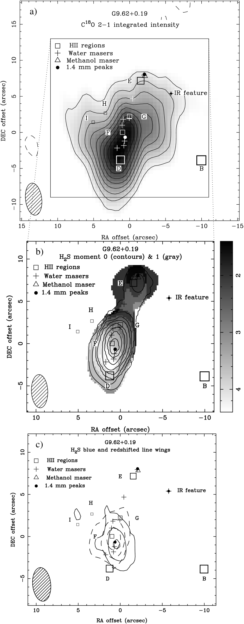
Figure 2: a) C¹⁸O 2$\rightarrow$1 integrated intensity towards G9.62. H ii regions are marked with open squares and water masers from Hofner & Churchwell (1996) are marked by plus signs. The IR feature of Persi et al. (2003) is marked by a plus sign with a small filled circle. The size of the open squares reflects the centimeter-wave flux density: a larger square represents a greater flux density. b) Contours of the zeroth moment (clipped at 2.0 Jy beam^-1) superimposed on a color-scale representation of the first moment (clipped at 2.5 Jy beam^-1). Contours begin at 6 Jy beam^-1 km s^-1 and increase in steps of 4 Jy beam^-1 km s^-1. The grayscale scale varies linearly between 1.4 km s^-1 (black) and 4.2 km s^-1 (white). The beam is marked by the hatched ellipse in the bottom left-hand corner of the image. c) Superposition of blue-shifted (solid contours) and red-shifted H₂S emission (dashed contours). Average emission over a 4 km s^-1 -wide range centered at $-$4 km s^-1 (blue) and 10 km s^-1 (red). Contours increase in steps of 0.36 Jy beam^-1 starting at 0.54 Jy beam^-1.

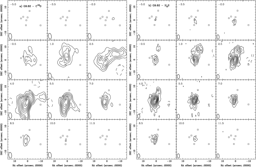
Figure 3: G9.62 channel maps of a) C¹⁸O and b) H₂S emission from $-$5 to 11.5 km s^-1 in steps of 1.5 km s^-1. Contours begin at 1.2/0.45 Jy beam^-1 and increase in steps of 0.8/0.30 Jy beam^-1 for C¹⁸O and H₂S respectively. H ii regions are marked by open squares. The beam is marked by the ellipse in the bottom left-hand corner of the image.

The C¹⁸O 2$\rightarrow$1 emission towards G9.62 defines a single elongated core encompassing components F and D (Figure 2a). Component E lies towards the edge of the integrated emission but does not stand out as a separate core. The emission shows a number of weaker extensions which do not appear to be associated with any of the known H ii regions. The overall distribution closely follows that of the C¹⁸O 1$\rightarrow$0 emission shown by Hofner et al. (1996). Channel maps (Figure 3a) reveal what may be the limb of a shell of gas defining the interface between the extended H ii region B and the molecular cloud. A velocity gradient exists from north to south (blue to red) as seen previously by Hofner et al. (1996) in their 1$\rightarrow$0 data.

The C¹⁸O spectra show self-absorption dips toward the center of the core. Comparing the total flux with the single-dish measurements of Hatchell et al. (1998b) show that our observations recover all of the C¹⁸O emission to within the calibration uncertainties. Therefore, it is likely that these dips are genuine and not a result of missing flux in the map. The presence of the self-absorption makes it difficult to reliably estimate linewidths, but away from the core center the typical linewidth is $\sim$4.0 km s^-1. There appears to be a weak red wing on the C¹⁸O spectrum toward component F, as also observed by Hofner et al. (1996). However, a map of the blue and redshifted emission does not show clear evidence for an outflow.

The total integrated H₂S emission in G9.62 also defines an elongated core (see Figure 2b), but it is clear that the denser gas traced by H₂S is concentrated toward components E and F with two clear maxima seen toward these sources. The emission also extends to cover components D and G but it is not possible to distinguish separate cores. The H₂S emission peaks coincide with the 1.4-mm continuum sources presented in Paper II. No H₂S emission is detected toward components B, C, H or I. No emission was detected toward the extended near-infrared feature discovered by Persi et al. (2003).

The H₂S lines tend to be broader than the C¹⁸O lines, indicating their formation in more turbulent regions closer to the center of the core, and are broadest at the position of component F with a full-width-at-half-maximum (FWHM) of 6.8 km s^-1. The FWHM linewidth at E is 3.1 km s^-1, 5.2 km s^-1 at G and 3.8 km s^-1 toward component D. The spectrum toward F shows both blue and redshifted wing emission, and a map of the blue-shifted emission between $-$6 and 0 km s^-1 reveals a well-defined lobe of emission slightly displaced from the center of core F. The redshifted gas (integrated between 8 and 13 km s^-1) defines a counterpart to the blue lobe, and is centered on component F: see Figure 2c. Most of the H₂O masers near G9.62F are redshifted, suggesting that they arise in the outflow. The outflow lobes do not show the same position angle nor do they peak at the same position as those seen in the HCO⁺ data of Hofner et al. (2001) but they are in the same sense: blueshifted gas to the SW, redshifted to the NE. The H₂S results therefore reinforce the interpretation that F is the hot core source and that it contains a young high-mass protostellar object.

Like the C¹⁸O, the H₂S data also delineate a clear velocity gradient along the major axis of the core, also seen previously by Hofner et al. 1996), shown in a grayscale representation in Figure 2b (although not so obvious from the channel maps in Figure 3b). The H₂S outflow emerges at an angle to the long axis of the core. The position angle of the outflow is 10.5 degrees east of north; that of the core is $-$13 degrees. (The position angle of the HCO⁺ outflow is 28 degrees.) The orientation of the blue and red lobes of the outflow defines a velocity gradient which is in the opposite sense to that seen along the major axis of the core, i.e. redshifted in the south and blueshifted to the north and west, further supporting our interpretation that the line wings arise in a bipolar outflow driven by an embedded source within F. Hofner et al. (2001) present arguments for the outflow being viewed pole-on. In this geometry it is unlikely that significant rotation can be detected. An alternative (and perhaps more likely) possibility is that the velocity gradient is due to the superposition of three cores (housing components D, F and G) which lie at different velocities. Higher angular resolution would enable this hypothesis to be tested.

While G9.62E is clearly detected in H₂S emission, no line wings are observed which implies that either it has yet to form an outflow or it has evolved beyond the outflow stage. Given its well-defined H ii region (stronger than F) and weaker dust emission than component F, it is likely that G9.62E is more evolved than G9.62F and has begun to clear away its parent core.

3.2 G10.47+0.03

G10.47+0.03 houses a group of four ultracompact H ii regions, three of which (A, B1 and B2) lie within a region 2 arcsec across (C98). C98 argue that the majority of the NH₃ (4,4) emission originates behind the three H ii regions, with component A being the least embedded. The ammonia peaks approximately 0.5 arcsec east of B1. The fourth H ii region, G10.47C, lies outside the area of ammonia emission. In this interpretation, the radio continuum sources are not deeply embedded within the hot core, instead lying close to the front surface.

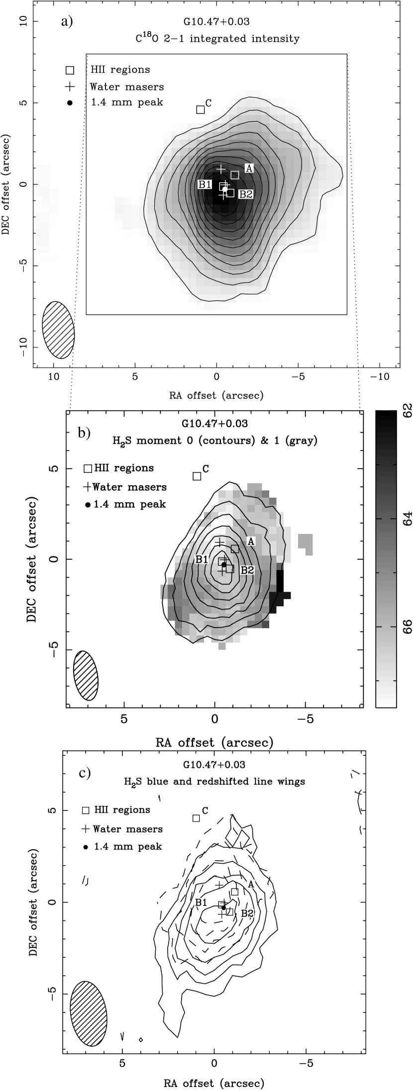
Figure 4: a) G10.47 moment zero contours (clipped at a flux density of 1.0 Jy beam^-1) superimposed on a grayscale of the first moment (clipped at 2.0 Jy beam^-1 to isolate the line core). Contours begin at 10 Jy beam^-1 km s^-1 increasing in steps of 10 Jy beam^-1 km s^-1. The peak is 78 Jy beam^-1 km s^-1. Ultracompact H ii regions are marked by open squares and water masers by plus signs. The beam is marked by the ellipse in the bottom left-hand corner of the image. b) G10.47 high velocity emission averaged over the velocity ranges 74 to 76 km s^-1 (red) and 58 to 60 km s^-1 (blue). Redshifted gas is shown by the dashed contours and blueshifted gas by the solid contours. Contour levels are the same for each lobe, beginning at 0.54 Jy beam^-1 in increasing in steps of 0.36 Jy beam^-1.

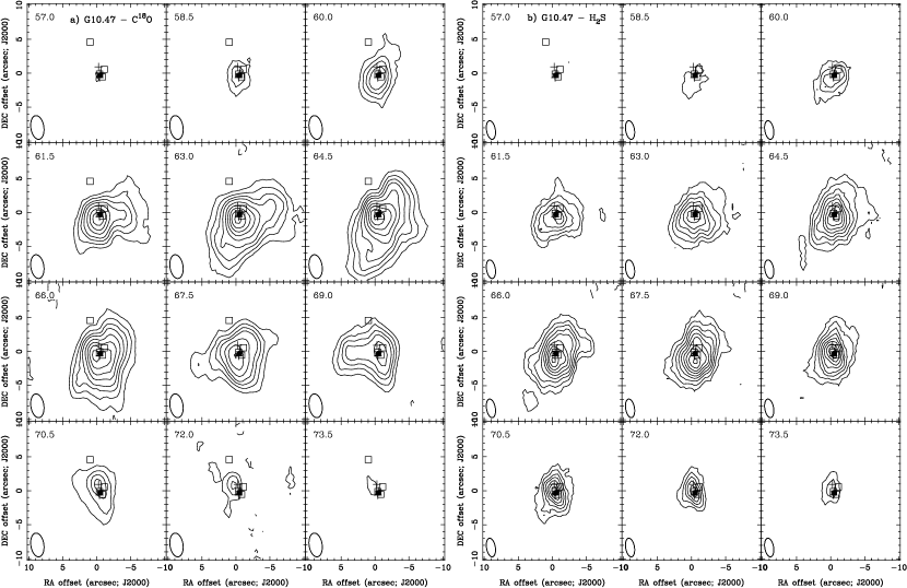
Figure 5: G10.47 channel maps of a) C¹⁸O and b) H₂S emission between 57 and 73.5 km s^-1. Contours begin at 0.6/0.75 Jy beam^-1 increasing in steps of 0.4/0.5 Jy beam^-1 for C¹⁸O and H₂S respectively. Symbols are as in Figure 4. The beam is marked by the ellipse in the bottom left-hand corner of the image.

The C¹⁸O emission (Figure 4a) defines a single compact core peaking on the H ii regions B1 and B2, with an extension to the west. No emission is detected toward component C. A number of features including the westward extension show up more clearly in the channel maps (Figure 5a). The westward extension covers the velocity range 61.5 to 64.5 km s^-1 (curving further north at 64.5 km s^-1), while between 64.5 and 69 km s^-1 a corresponding feature exists in the south-east to east, with a well-defined tongue of emission extending to the east at 69 km s^-1. Such features could represent a bipolar outflow, or a rotating (fragmented) core. We rule out outflow since the spectra to the east and west of center peak at different velocities, and thus the east and west extensions are not due to high-velocity line wings. Therefore it seems likely that these features define a gradient in the bulk of the core, and may represent smaller and less-massive individual cores.

The C¹⁸O spectra are single peaked across the entire region, and broadest at the position of the hot core. The linewidths at the positions of the east and west components are much narrower than toward the hot core ($\sim$3 km s^-1). Comparing our data with those of Hatchell et al. (1998b) again shows that we detect all of the C¹⁸O flux to within the calibration uncertainties.

The H₂S line is only detected in emission towards G10.47 and we do not see the same bow-shape seen in the ammonia of C98 caused by absorption against the H ii regions. The integrated H₂S emission (Figure 4b) shows a single-peaked core elongated in a NW-SE direction at the lowest contours, but twists to a NE-SW direction in the highest contours, encompassing the UCH ii regions, B1 and B2. This suggests that there are two separate cores containing B1 and B2 which we are unable to resolve. Like C98, we also do not detect any molecular line emission toward G10.47C.

The brightest emission lies slightly south of B1/2, and extends further south by $\sim$2 arcsec, consistent with elongation in dust continuum (Paper II). The spectra toward each of the H ii regions are flat-topped which could be due to either the presence of two velocity components which we are unable to resolve (perhaps from an expanding shell) or high optical depths in the H₂S line. In our discussion below (Section 4.1) we conclude that the H₂S is most likely to be optically thick.

The H₂S covers a velocity range from 58 to 74 km s^-1  a similar range to the C¹⁸O. Unlike the other sources in this sample, the H₂S line does not show the same clear high-velocity wings (Figure 1). However, the H₂S lines toward G10.47 are the broadest in our survey with a peak FWHM of 10.5 km s^-1. From channel maps it is possible to distinguish two velocity components, although these do not correspond to any of the kinematic features of the C¹⁸O data. The first component extends in the NE–SW direction and covers the range 61 km s^-1 to 73 km s^-1. A second component extends NW–SE which traces material between 59 and 70 km s^-1. The NE-SW velocity component is also seen in NH₃ (4,4) of C98. A secondary peak is observed at (3,$-$7) arcsec offset over the velocity range 65 to 67 km s^-1, coincident with one of the C¹⁸O cores desrcibed above.

While the H₂S spectra do not show clear high-velocity line wings, the extreme red and blue shifted emission does show a slight north-south separation, although it is less than one beam diameter (Figure 4c). The center of this ‘outflow’ lies $\sim 1^{\prime\prime}$ north of the the 1.4-mm continuum peak and the UCH ii regions B1 and B2. The fact that all the water masers are aligned on a north-south axis lends support to an outflow interpretation. The outflow interpretation gains further support from the fact that Olmi et al. (1996) detected a velocity gradient in ¹³CO consistent with a north-south outflow (in the same sense as we observe in H₂S), as well as an east-west velocity gradient in CH₃CN, i.e. perpendicular to the proposed outflow (although see § 5.2.1 below). The small offset between the lobes means that we have not resolved a flow direction, or that there is no outflow and we are be seeing the front and back surfaces of an expanding shell of gas centered on the H ii regions. We therefore conclude that there is only weak evidence for either outflow or rotation toward G10.47.

3.3 G29.96$-$0.02

The ultracompact H ii region in G29.96$-$0.02 shows a classic cometary shape (Wood & Churchwell 1989), which is also evident in our 2.7 and 1.4-mm continuum data (Paper II). C98 also observed G29.96 in ammonia (4,4) and detected a single peak coincident with a group of water masers, but offset from the H ii region. Dust emission peaks at the position of the ammonia and water masers (Olmi et al. 2003; Paper II) confirming the location of the hot core.

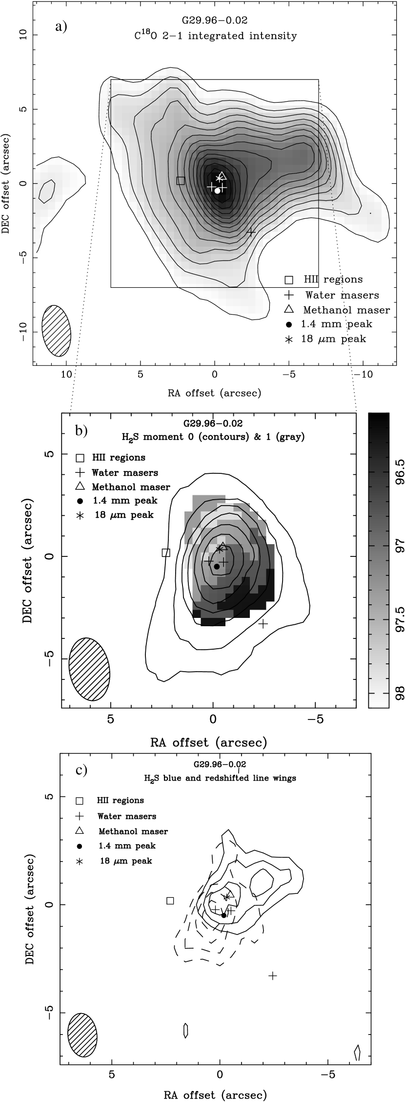
Figure 6: a) Contours of zeroth moment superimposed on the first moment grayscale image (clipped at a flux density of 2 Jy beam^-1 to isolate the line core). Note the SW–NE gradient in the first moment data perpendicular to the direction of the outflow lobes, suggestive of a rotating core. b) Red-shifted (dashed contours) and blue-shifted (solid contours) H₂S emission averaged over a 4-km s^-1-wide interval centered at 90 km s^-1 (blue) and 106 km s^-1 (red). The 18-$\mu$m peak is almost coincident with the methanol maser (De Buizer et al. 2002) which lies within the blue lobe of the outflow. Contours for each lobe begin at 0.1 Jy beam^-1 and increase in steps of 0.1 Jy beam^-1. The beam is marked by the ellipse in the bottom left-hand corner of the image.

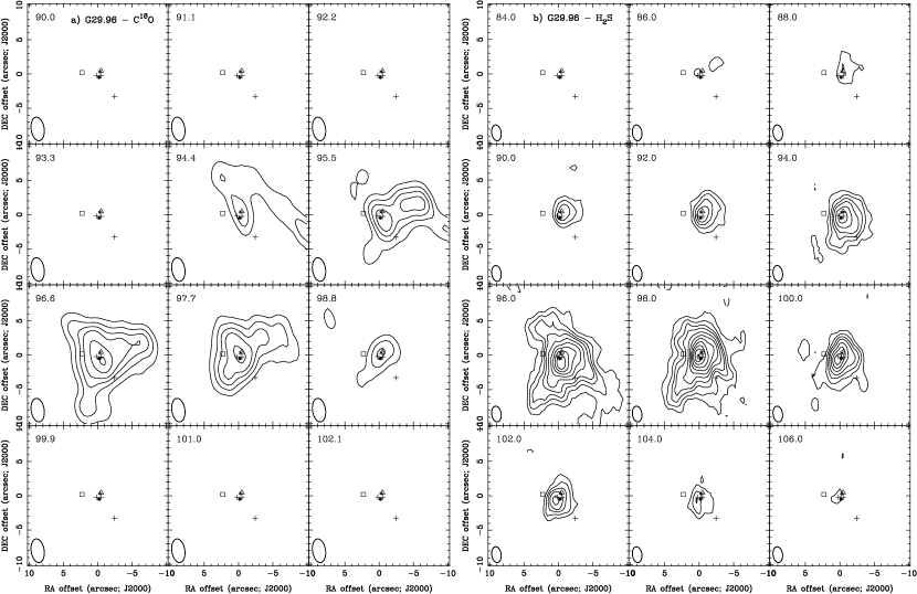
Figure 7: G29.96 channel maps of H₂S emission from 90 to 102.1 km s^-1 (C¹⁸O) and 84 to 106 km s^-1 (H₂S) in steps of 1.1/2 km s^-1(C¹⁸O/H₂S resepctively). Contours begin at 1.2/0.3 Jy beam^-1 and increase in steps of 0.8/0.2 Jy beam^-1 for C¹⁸O and H₂S respecetively. The 1.4-mm continuum peak is marked by a filled circle, the position of the UCH ii region is marked by an open square, water masers are marked by plus signs, the methanol maser group of Minier et al. (2002) are marked by an open triangle. The beam is marked by the ellipse in the bottom left-hand corner of the image.

The C¹⁸O emission toward G29.96 defines an extended core with multiple peaks (Figure 6a). There is general good agreement with the 1$\rightarrow$0 data of Olmi et al. (2003), although they do not detect the westward ridge we see in our data. The C¹⁸O emission shows a well-defined edge extending from north-east to south-west, which is likely associated with the boundary between the molecular cloud and the ultracompact H ii region. This is seen more clearly in the channel maps, Figure 7a. This fact indicates that the hot core and the ultracompact H ii region are embedded within the same molecular cloud. The lone water maser $\sim$4.5^′′ to the SW does not appear to be associated with any other peaks in either the C¹⁸O or H₂S emission.

The C¹⁸O emission peaks on the hot core, decreasing in intensity to the west, where at least two further cores can be discerned. These cores have not been resolved by any previous observations. There is a very slight velocity gradient along this ridge with the more distant core being marginally blue-shifted relative to the hot core (spectra peak at 96.8, 96.5 and 96.1 km s^-1 from east to west).

The C¹⁸O lines are relatively narrow across much of the source, peaking at the hot core position. G29.96 has the smallest range of C¹⁸O emission of our sample of sources, covering only 5 km s^-1(Figure 7a). The linewidths decrease along the westward ridge away from the hot core (4.0, 3.5 and 3.2 km s^-1 for the hot core, W1 and W2 respectively). Once again, there is good agreement between our C¹⁸O flux and the single-dish measurement of Hatchell et al. (1998b).

The integrated H₂S emission shows a single maximum coincident with 1.4-mm continuum peak (Figure 6b). Channel maps show that the H₂S is extended over a region $\sim 15^{\prime\prime}$ in diameter and appears to wrap around the head of the UCHII region (Figure 7b), in a similar manner to the C¹⁸O. The H₂S emission in G29.96 is the most extensive of all our four sources, and shows extensions to the west and south-west which may be further individual cores.

The H₂S spectra (Figure 1) show strong line wings extending to $\pm$10 km s^-1 across a wide area. Redshifted wings are seen in the south-east while blue-shifted wings extend to the north-west. Figure 6c shows the integrated red and blueshifted emission and clearly shows the spatial bipolarity of an outflow. The outflow center appears to lie closer to the ammonia peak of C98 than our 1.4-mm peak. This may indicate that there are multiple sources within the G29.96 hot core: higher resolution observations are clearly needed. The orientation of the blue lobe is along line of methanol masers seen by Minier, Booth & Conway (2002). The methanol masers are also blueshifted, increasingly blueshifted with distance from the outflow center.

Figure 6b also shows an image of the first moment of the H₂S emission (clipped at a level which excludes the wing emission), revealing a velocity gradient along a SW to NE axis, blue-shifted in the SW and redshifted toward the NE. There is evidence of this same gradient in the C¹⁸O data as well. Figure 7a shows that the C¹⁸O peaks to the SW of the hot core at 95.5 km s^-1 and to the NE at 97.7 km s^-1. It is tempting to interpret this as rotation of the hot core, especially since the gradient is observed to be perpendicular to the outflow direction. However we regard this conclusion as somewhat tentative and clearly requires further observations of high-density tracers which are not contaminated by outflow. Under the assumption that we are detecting rotation the velocity gradient is $\sim$11 km s^-1  pc^-1, corresponding to a rotation period of $8.9\times 10^{4}$ yr.

3.4 G31.41+0.31

The region associated with G31.41+0.31 houses an ultracompact H ii region along with a diffuse shell of extended radio continuum emission (Wood & Churchwell 1989). Hofner & Churchwell (1996) detect a group of 8 water masers, none of which coincide with the UCH ii region. However, the ammonia observations of C98 reveal a compact core of molecular gas clearly coincident with the water masers, but with no associated centimeter continuum emission.

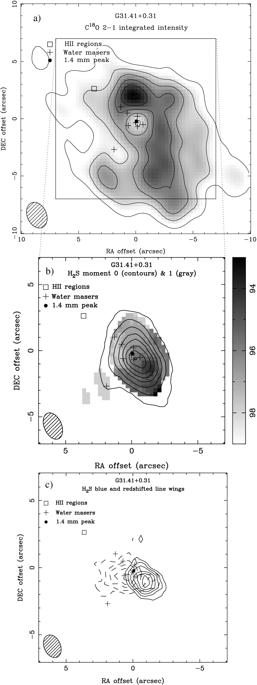
Figure 8: a) Moment zero (integrated intensity, clipped at 0.5 Jy beam^-1) contours superimposed on grayscale of the first moment image (clipped at 1.5 Jy beam^-1). Contours start at 4 Jy beam^-1 km s^-1, increasing in steps of 5 Jy beam^-1  km s^-1. The peak is 41 Jy beam^-1 km s^-1. Grayscale is linear from 92.5 (blue) to 98.9 km s^-1 (red) as shown on the sidebar. b) G31.41 redshifted contours (red) and blueshifted contours (blue) averaged over a 4-km s^-1-wide interval centered at 89 km s^-1 (blue) and 105 km s^-1 (red). For each lobe, the contours begin at 0.2 Jy beam^-1 and increase in steps of 0.1 Jy beam^-1.

Our C¹⁸O emission shown in Figure 8a defines an elongated core, mostly oriented north-south but with a clear contribution from a diffuse, more extended component oriented NE-SW. Most notable is the fact that the C¹⁸O does not peak at the hot core position; in fact the hot core is seen as a local minimum in the C¹⁸O emission. A comparison of our data and the JCMT measurement of Hatchell et al. (1998b) shows that we only detect of order 70% of the C¹⁸O flux. It may be that the C¹⁸O is not strongly peaked on the hot core position and is thus filtered out by our interferometric observations. Alternatively, the brightness temperature of the continuum emission may be sufficiently high (at 27.5 K for the naturally-weighted data) that the C¹⁸O is simply not detectable above this level. There are a number of peaks evident in the integrated map, although it is not certain if they represent independent cores given that some of the flux is missing from the image.

Channel maps reveal the structure of the core. Figure 8a shows the presence of a clear velocity gradient along the major axis of the C¹⁸O core, blue-shifted in the south and red-shifted to the north. The individual peaks seen in the integrated intensity map are clearly seen in the channel maps.

Figure 8b shows that the integrated H₂S emission is centered on the 1.4-mm and ammonia emission, with the water masers mostly lying along an axis parallel with the observed extension of the H₂S core. The first moment image also shown in Figure 8b shows a weak velocity gradient along the core (in the same sense as the larger-scale C¹⁸O gradient), which is tempting to interpret as rotation. The high-velocity wing emission (shown in Figure 8c) is predominantly east-west in orientation. A position-velocity cut along the core shows the velocity gradient more clearly (see § 5.2 below). We need further observations of complementary tracers to isolate one velocity component from the other. We note that the lower-resolution HCO⁺ 1$\rightarrow$0 and SiO 2$\rightarrow$1 observations of Maxia et al. (2001) show the same distribution of red- and blueshifted high-velocity gas, supporting the outflow interpretation. The water masers appear to be associated with the outflow since many of the maser spots are red-shifted.

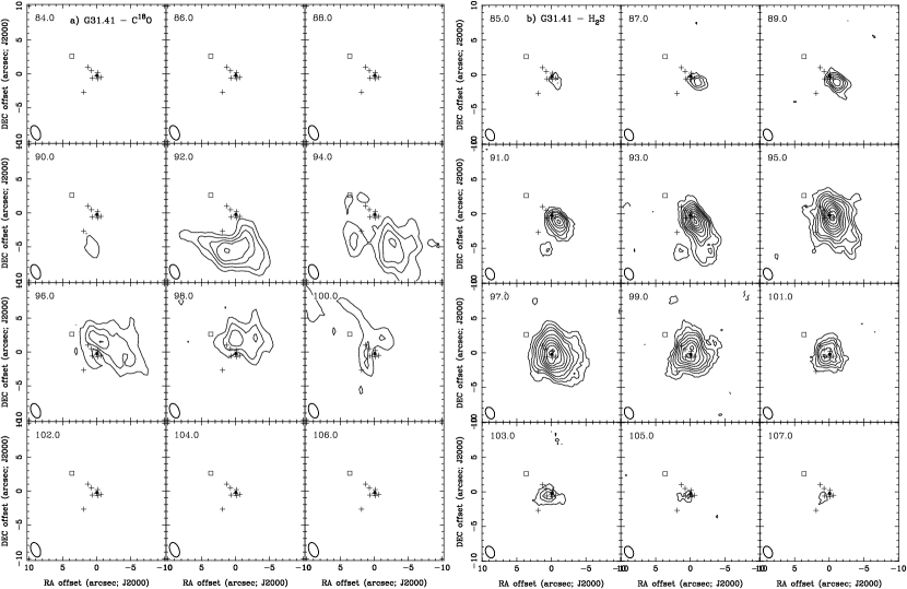
Figure 9: G31.41 channel maps of a) C¹⁸O and b) H₂S emission from 85 to 107 km s^-1 increasing in steps of 2 km s^-1. Contours begin at 0.45/0.3 Jy beam^-1 and increase in steps of 0.3/0.2 Jy beam^-1 for C¹⁸O and H₂S respectively. Plus signs mark the location of water masers from Hofner & Churchwell (1996), the position of the UCH ii region is marked by an open square and the filled circle marks the position of the 1.4-mm continuum peak. The beam is marked by the ellipse in the bottom left-hand corner of the image.

Channel maps (shown in Figure 9b) show that the H₂S emission is largely extended in the same NE-SW direction at all blue-shifted velocities. At the south end of the core, two secondary peaks show up at 91 to 93 km s^-1, and it may be these components which bias the first moment image toward greater blue-shifted velocities in this regions. These may represent separate independent cores since our C¹⁸O data show an extended maximum toward these positions (and at the same velocity), as do the HCO⁺ data of Maxia et al. (2001). The H₂S spectra show varied line shapes across the core, with clear blue- and red-shifted wing emission toward some positions, and double-peaked line profiles toward the center of the core. However, as described above for G10.47, the double-peaked profiles may be due to self-absorption of an optically thick line.

4 Analysis: Hot core masses and outflow parameters

In this section we describe our analysis of the data in order to derive various physical parameters of the hot cores. We have made two-dimensional gaussian fits to the integrated-intensity images to derive source dimensions and intensities. In most cases a gaussian fit was a good representation of the observed emission. The deconvolved source dimensions were estimated assuming a gaussian geometry: these are the values listed in Table 2. The mean linewidth was derived from gaussian fits to spectra toward each source (also given in Table 2). Next, virial masses were calculated assuming that each core can be approximated to a sphere of constant density. If the density falls off with radius then, for typical power-law indices, the virial masses will be smaller by up to 40 per cent (see e.g. MacLaren, Richardson & Wolfendale 1988). H₂ column and volume densities were calculated from these virial masses, again assuming constant density spheres. For C¹⁸O we also calculated a total H₂ mass based on the integrated intensity since the abundance is assumed to be well known (2$\times$10^-7). These derived values are listed in Tables 3 and 4.

4.1 Masses and column densities

There is generally good agreement between the virial mass estimates from the H₂S data and those derived from the C¹⁸O. In the C¹⁸O data, G29.96 has the lowest virial mass and G10.47 the largest. G10.47 also has the largest H₂S-derived virial mass, although now G9.62E has the lowest value. With the exception of G29.96, the C¹⁸O virial masses are larger than the H₂S masses, a result of the larger core size measured in the C¹⁸O data. As expected, the H₂S is tracing denser gas than the C¹⁸O, and yields larger estimates of the H₂ column density on account of the smaller source size.

The molecular hydrogen column densities inferred from the H₂S virial masses are exceedingly high. In particular, G10.47 has the highest column density in our sample at $6\times 10^{24}$ cm^-2, corresponding to a visual extinction of 12 600 magnitudes. Even at mid-infrared wavelengths, the extinction remains significant. Using the values given by Mathis (1990), this H₂ column density corresponds to an extinction of 270–300 magnitudes at 20 $\mu$m. The extinction extrapolated to 1.4 mm is only 0.17–0.20 magnitudes, or essentially optically thin ($\tau\sim$0.25). However, since the grain properties in the dense regions toward these hot cores can be different to those in the interstellar medium, the actual submillimeter optical depth could be higher. The H₂S virial masses imply a mean density in the four hot core sources of order $10^{7}$ cm^-3, in good agreement with values derived by Cesaroni et al. (1994).

We have calculated the C¹⁸O and H₂S column density toward the hot core positions in each source (plus component E in G9.62), shown in Tables 3 and 4. We have assumed the emission to be optically thin, and that the level populations can be characterized by a single excitation temperature. The choice of excitation temperature is not constrained since we only have a single transition. For C¹⁸O we have assumed values between 16 (equal to the energy of the $J$=2 level to obtain the minimum value: Macdonald et al. 1996) and 125 K (a reasonable upper limit based on ammonia and CH₃CN estimates, e.g. Cesaroni et al. 1994; Olmi et al. 1996). Using the H₂ column densities derived from the C¹⁸O virial masses to estimate an abundance of C¹⁸O yields values smaller than the canonical value of $2\times 10^{-7}$ for G10.47 and G31.41, but in reasonable agreement for G9.62 and G29.96. Therefore, either the C¹⁸O towards G10.47 and G31.41 is not optically thin, or we are resolving out a significant portion of the C¹⁸O emission. Since the agreement with previous single-dish observations is good for G10.47, we conclude that the C¹⁸O is optically thick in this source. The C¹⁷O and C¹⁸O data of Hofner et al. (2000) show that the C¹⁸O 2$\rightarrow$1 line has moderate optical depth ($\sim$1–2) in an 11″ beam for all our sources. However, it is likely that the missing flux contributes to the poor agreement for G31.41. We have also calculated masses from the integrated intensity maps, assuming the standard C¹⁸O abundance and optically thin emission. Table 3 shows that there is good agreement between the masses calculated in this way and the virial masses for G9.62 and G29.96. The integrated masses are much lower than the virial masses for G10.47 and G31.41, which is probably due to the effects discussed above.

The observed H₂S line brightnesses yield minimum excitation temperatures of 18 to 40 K (Figure 1). However, a strict lower limit for H₂S can be obtained assuming that $T_{\rm ex}=2E_{\rm u}/3k=56$ K (Macdonald et al. 1996) where $E_{\rm u}$ is the energy of the upper level, equivalent to 84 K in temperature units for the H₂S 2(2,0)$\rightarrow$2(1,1) transition. However, the exact value is relatively unimportant as the derived H₂S column density changes by only 50 per cent over the temperature range 30 to 250 K. Therefore, our choice of excitation temperature results in only a small uncertainty in our calculations, and lower than the uncertainty due to unknown optical depth. As a result, we only list a minimum value in Table 4. Examining the line intensities we see that for an excitation temperature of 56 K, the lines in G10.47 and G31.41 are not optically thin ($\tau\sim 1$, and higher for lower excitation temperature).

The H₂S column density varies from $3\times 10^{15}$ cm^-2 toward G9.62E to $4.1\times 10^{16}$ cm^-2 toward G10.47. If we assume that the virial masses calculated above are accurate representations of the mass of the region containing the H₂S then we can estimate the abundance of H₂S in each source. This yields column-averaged H₂S abundances of $1.2$–$6.8\times 10^{-9}$ relative to H₂. Bearing in mind the fact that the virial masses are probably upper limits, and the fact that the H₂S column density is a lower limit, these abundances should themselves be regarded as lower limits, although they are in good agreement with estimates from Hatchell et al. (1998b) and van der Tak et al. (2003).

4.2 Comparison with previous estimates

The first comparison we make is with our own BIMA continuum data presented in Paper II. To estimate the dust masses we assumed an dust emissivity of 0.018 cm² g^-1 at 1.4 mm (Ossenkopf & Henning 1994) and a temperature between 50 and 250 K. This yields dust masses in the range 17 to 94 M_⊙ (G9.62F), 151 to 824 M_⊙ (G10.47), 36 to 198 M_⊙ (G29.96) and 156 to 850 M_⊙ (G31.41) with the larger values corresponding to the lower temperatures. In all cases, the C¹⁸O and H₂S are considerably more extended than the dust emission, with FWHM dimensions typically twice as large as those of the dust cores.

One the whole, there is reasonable agreement between the dust masses and the virial masses for both C¹⁸O and H₂S, at least for the lower dust temperatures. If the dust is indeed as hot as 250 K, however, then the discpreancy between the dust and molecular line estimates can be large, ranging from a factor of 3 to more than an order of magnitude difference. If the dust emission is optically thick, we will underestimate the dust masses. Earlier we estimated a dust optical depth of 0.25 at 1.4 mm, which would lead to us underestimating the mass by only 10% or so. On the other hand, the H₂S is clearly associated with outflow motions, which artifically raises the virial mass (due to increased linewidths), leading to the observed large discrepancy between the mass estimates. Using the (lower) mass estimates from the dust emission to derive H₂ column densities will lead us to derive higher values for the H₂S abundance. Performing this calculation yields H₂S abundances a factor of 3–5 higher than given in Table 4 (again dependent on the assumed dust temperature).

The H₂S virial masses for both component G9.62E and G9.62F are in good agreement with the masses derived from C¹⁸O by Hofner et al. (1996), and our C¹⁸O virial mass agrees well with their total mass for E and F. Since we measure a larger linewidth for our H₂S data (7.8 km s^-1 compared with 4.4 km s^-1 for ammonia), our estimate of the virial mass for F is correspondingly higher than the Cesaroni et al. (1994) value although the sizes are in good agreement. Consequently, we also derive higher densities. Our larger linewidth is a reflection of the presence of the H₂S in the outflow; ammonia is therefore not present or excited in detectable quantities in the outflow.

Mass estimates for the other three sources vary considerably. Virial masses derived from the ammonia (4,4) line (Cesaroni et al. 1994) tend to be $\sim$5 times smaller than our values, largely due to the higher H₂S linewidth and larger extent in C¹⁸O. Tracers employed at 3 mm by Maxia et al. (2001) and Olmi et al. (2003) yield estimates similar to what we derive. Maxia et al. (2001) use a smaller dust emissivity that we have employed; consequently we revise their estimates derived from 3-mm dust continuum downwards by a factor of $\sim$4 to give $\sim$700 M_⊙ and 350 M_⊙ for G29.96 and G31.41 respectively. Olmi et al. (2003) estimate a mass of 1200 M_⊙ for G29.96 from C¹⁸O, larger than our estimates (Table 3, 4).

Submillimeter dust continuum models constructed by Hatchell et al. (2000) for G10.47 and G31.41 have a constant density core at the center which has a mass of 3000 M_⊙ within a radius of 0.06 pc, somewhat larger than our estimates for a similar-sized region.

The dimensions we derive for G9.62F are very similar to what Cesaroni et al. (1994) determine from their ammonia data. In G10.47, G29.96 and G31.41 the size of the hot core derived from the H₂S emission is larger than that derived from the ammonia observations of Cesaroni et al. (1994) and C98. C98 showed that the optically thicker main hyperfine lines of ammonia yielded a larger source size than the satellites. Since we find that the H₂S emission is probably optically thick, it seems plausible that the larger source size is due to a high optical depth in the H₂S lines. Alternatively, our BIMA observations may be more sensitive to the distribution of H₂S relative to the VLA observations of ammonia (Cesaroni et al. 1994). A third (and perhaps most likely) possibility is that the ammonia (4,4) line simply traces warmer gas than the H₂S as the energy of the upper level is 84 K for the H₂S while that of the NH₃ (4,4) line is 201 K.

4.3 Outflow parameters

In Table 5 we list the derived properties of the outflows toward each source, including the mass of H₂S-emitting gas. If we assume an abundance, then we can estimate the mass of swept-up material in the outflows from each source on the condition that the H₂S is well-mixed with the molecular hydrogen. The H₂S abundance is not well known in molecular clouds, and even less well known in outflows. In the previous section, we derived column-averaged abundances of order $10^{-9}$, which are probably lower limits. In other work, Minh et al. (1991) derived values close to $10^{-8}$ in a number of high-mass star-forming regions, and as high as $10^{-6}$ in Orion (Minh et al. 1990).

For the gas in the outflow, we assume an abundance of $10^{-7}$ relative to molecular hydrogen as it lies in the middle of the range of values derived by Minh et al. (1990, 1991), and $10^{-7}$ is used as an initial value for the gas-phase H₂S abundances in the majority of chemical models (e.g. Rodgers & Charnley 2003, Wakelam et al. 2004). If the H₂S abundance is as high as $10^{-6}$, then we derive minimum outflow masses of 0.4 M_⊙, values typical of relatively low-mass stars. On the other hand, if we assume smaller values then the mass estimates will increase to very high values (40 M_⊙ per lobe). Therefore, we regard our assumption of $10^{-7}$ for the H₂S abundance as providing reasonable lower-limits to the outflow parameters, although CO observations are desireable to determine these parameters with greater certainty.

It appears that for all our sources several solar masses of material has been swept up, typically $\sim$4 M_⊙ in each lobe. Since we have neglected emission close to the line center, the true mass of each outflow is probably higher. Even so, given the mass estimates in Table 5, it is clear that these outflows are being driven by massive protostars since they compare favorably with a number of measurements of larger, more well-developed flows from massive YSOs (e.g. Gibb et al. 2003; Shepherd et al. 1998).

If we assume that the outflow masses we derive are a sufficiently accurate reflection of the true masses, we can also estimate other properties of the outflows such as the momentum and energy. We assume that the characteristic outflow velocity is $v_{\rm out}=v_{\rm max}/2$ so that the momentum, $p$, is simply $mv_{\rm out}$, and the energy is $E_{\rm K}=mv_{\rm out}^{2}/2$. Similarly, we assume the outflow ‘size’ ($r_{\rm out}$) to be half the mean diameter of the outflow lobes. The dynamical ‘age’, $t_{\rm dyn}$, is calculated from $r_{\rm out}/v_{\rm out}$, with outflow force and mechanical luminosity calculated as $p/t_{\rm dyn}$ and $E_{\rm K}/t_{\rm dyn}$. Table 6 lists the values thus calculated. The average value for each outflow is given; the total momentum, energy, etc., will be a factor of two higher. All the values are consistent with the outflows being driven by relatively massive YSOs (c.f. Shepherd & Churchwell 1996), although the choice of H₂S abundance clearly affects our final numbers. However, we wish to point out that since we are not sensitive to the highest-velocity gas (the velocity extent is quite low) the momentum and energy for each outflow will be seriously underestimated. High-$J$ CO observations are desirable in order to better constrain the flow energetics.

5 Discussion

H₂S has only been previously observed in single-dish observations of these sources. Since we are able to resolve the structure of the H₂S emission we can now discuss our observations in the context of physical and chemical models of hot cores.

5.1 H₂S in hot cores: distribution and abundance

Hatchell et al. (1998a) estimate the H₂S column density toward all four of our target sources from single-dish observations of the same transition (and assuming the same excitation conditions) as we present here. These single-dish column densities are typically a factor of 20 lower than the column densities we derive, due to the brightness temperature being diluted by the 22-arcsec JCMT beam. Thus the filling factor for the JCMT observations is $\sim$1/20, which predicts a source size of order 5″, very similar to what we observe (Table 4).

In the absence of any other input, chemical models of hot cores start with a gas-phase H₂S abundance of around $10^{-7}$ based on the observations of Minh et al. (1991), and more recently on the ISO results which place an upper limit of $10^{-7}$ on the solid H₂S abundance (van Dishoeck & Blake 1996). For example, Rodgers & Charnley (2003) follow the evolution of chemical abundances in centrally-heated cores assuming two different models for the evolution of the physical parameters of the core. Rodgers & Charnley suggest that their static model is more appropriate for massive cores, and show that the abundance of H₂S is initially high and decreases rapidly with time. At early times ($<10^{4}$ yr) H₂S appears to have a uniform abundance across the core, falling off at an outer radius which increases with time, reaching 0.01 pc at $10^{4}$ yr (the outer radius of their model is 0.03 pc). The typical abundance for H₂S in these models is a few $\times 10^{-8}$ to $10^{-7}$, falling off rapidly with radius at late times (although it rises again in the outer regions of the core). Inspection of their predicted column densities shows that only at late times (at $10^{5}$ yr and beyond) does the H₂S column density fall below $10^{16}$ cm^-2. Simultaneously, the size of the hot core in ammonia is at least a factor of two smaller, purely as a result of the chemistry. This appears to be another factor which can account for the fact that these hot cores appear to be smaller in the ammonia images of C98 than in our H₂S.

We note that the hot core models predict H₂S abundances at least an order of magnitude greater than the values we calculate (Table 4). As discussed elsewhere in this paper, it is likely that a combination of high optical depth and an overestimated mass from the virial theorem can account for this discrepancy. Since ammonia is well studied on similar scales in hot cores, we can examine the NH₃/H₂S abundance ratio. Using the ammonia column densities given by Cesaroni et al. (1994) we derive ratios [H₂S/NH₃]=2–8$\times 10^{-3}$. However, in the models of Rodgers & Charnley (2003), this ratio never falls below unity except at late times ($10^{5}$ yr). The simplest explanation for the observed ratios is that the H₂S lines have significant optical depth leading to vastly underestimated H₂S column densities.

5.2 Hot core dynamics: outflow and rotation?

The data we present here appear to trace two kinematic components. The first is outflow traced by the H₂S. The second is a velocity gradient more or less perpendicular to the outflow and is probably rotation, seen in both C¹⁸O and H₂S. The outflow evidence is clear: spatially bipolar lobes of red- and blueshifted gas. The rotation interpretation is ambiguous, especially in light of the likely fragmented nature of the G9.62 core and the more obvious outflow signature in the H₂S. However, given the good agreement between the C¹⁸O and H₂S gradients across each core, the rotation interpretation seems more tenable. In Figures 10 to 13 we show selected position-velocity (PV) cuts across each of the H₂S data cubes for each of the hot cores (along the long axis of the core and along the outflow axis where defined). In three of the four sources clear velocity gradients are present. Only G10.47 (Figure 11) does not show a velocity gradient. The observed velocity gradients tend to be linear along the long axis of the core, although they typically only extend for a couple of beamwidths. (However, we note that it is possible to distinguish velocity gradients on scales smaller than a beam: e.g. Olmi et al. 1996.) It is clear that the velocity gradients do not directly show evidence for Keplerian rotation; indeed given the massive cores within which the central stars are embedded such a result would be surprising since a Keplerian rotation law only strictly applies for a dominant point mass (although it may be true that the velocity field is locally Keplerian). Furthermore, if the observed emission is optically thick (as concluded above) then regardless of the intrinsic velocity field, the observed velocity gradient will be linear.

However, even if the emission is not optically thick, our finite beamsize prevents us from directly observing a Keplerian rotation curve, instead smoothing out the central region into a linear gradient (see Richer & Padman 1991). Therefore, we caution against over-interpreting these PV data, especially since the emission closest to the center is heavily contaminated by the high-velocity emission from the outflow. At best we can only conclude that in the cases of G9.62, G29.96 and G31.41 our C¹⁸O and H₂S data show evidence for velocity gradients along the long axis of the hot core, but not what form the velocity law takes.

If we assume the linear velocity gradients are due to uniform rotation then we can estimate rotation periods, and then the masses required to bind the motions. For each of the three sources with clear velocity gradients (G9.62F, G29.96 and G31.41), the rotation periods for each core is similar at 1–2$\times 10^{5}$ yr. Using the core dimensions shown in Table 4 these periods require binding masses of only 15, 60 and 154 M_⊙ (for G9.62F, G29.96 and G31.41 respectively). These masses are all less than both the virial and dust-derived masses and so that the cores are rotationally bound, and may even be still collapsing. The velocity gradients along the outflow axes are larger and imply binding masses of 810, 2800 and 2360 M_⊙ respectively, all much larger than the virial masses given in Tables 3 and 4. Therefore the motions along the outflow axes are not bound to the hot cores.

An interesting feature of the G31.41 PV diagram is that the H₂S emission farthest from the center does not lie at the rest velocity. This indicates that the H₂S is not very abundant at these distances from the hot core and falls below our detection threshold. From Figure 13 we can therefore determine an outer radius of the hot core of $\sim$5 arcsec or 0.19 pc ($5.9\times 10^{17}$ cm).

5.2.1 An outflow origin for methyl cyanide?

Comparing our results with those of Beltrán et al. (2004) for G31.41, we find that our outflow direction is closely aligned with the long axis of their methyl cyanide emission, which they interpret as a rotating disk or toroid. Their interpretation was a natural conclusion given the example of IRAS 20126+4104 (Cesaroni et al. 1999) which shows a clear disk-like component for the CH₃CN emission. This ambiguity highlights the kind of problems faced when studying hot cores. However, we believe that our C¹⁸O and H₂S data display clear evidence for both outflow and (in two cases) velocity gradients perpendicular (or close to) to the axis of the outflow. The simplest interpretation for these gradients is rotation of the core. The distribution of our H₂S (and 1.4-mm continuum) data closely matches that of the NH₃ (4,4) of C98. This leads to the interesting conclusion that Beltrán et al. (2004) have actually detected CH₃CN in the outflow from G31.41. Further support comes from the CH₃CN observations of G29.96 by Olmi et al. (2003) which are also consistent with emission from an outflow since the velocity gradient is extremely high (higher than we detect with our H₂S data, thus requiring an even higher binding mass) and oriented mostly along the same direction as our outflow. It is interesting to compare the methyl cyanide and H₂S results. H₂S is clearly not confined to the outflow. On the other hand, it seems as if the CH₃CN in these sources is dominated by an outflow component, suggesting that it is perhaps shock chemistry that is playing a greater role in the formation of methyl cyanide. Clearly further high-resolution observations are necessary in order to explore this further.

5.3 Embedded sources in hot cores

The primary result from these observations is the confirmation that outflows emanate from some hot cores, including all four of the targets in our sample. Furthermore the images of the high-velocity emission show that these outflows appear to be collimated; in other words, unlike many ultracompact H ii regions, they are not spherical shells driven by the expansion of a symmetric stellar wind. This has important implications for the formation of massive stars and implies the presence of a collimation mechanism. In the case of low-mass stars, this is now widely believed to be a rotating circumstellar disk (Ouyed, Clarke & Pudritz 2003; Königl & Pudritz 2000). Explanations of outflows from more luminous protostars invoke a wider-angle contribution from a stellar wind (Shepherd et al. 1998; Richer et al. 2000), although a disk is still believed to play an important role in at least initially collimating the outflow.

Clearly we cannot determine whether circumstellar disks exist around these outflow sources with the current observations. However, we can examine whether the ambient medium has sufficient turbulent pressure to act as a collimating agent for the flows. Assuming a single driving source we may equate the momentum flux from the wind/outflow (assumed to be initially isotropic) with the turbulent back-pressure of the ambient medium:

$$\rho\sigma_{\rm 1D}^{2}=\frac{\dot{p}}{4\pi r^{2}}$$ (1)

where $\rho$ is the ambient density, $\sigma_{\rm 1D}^{2}$ is the 1-dimensional velocity dispersion ($=\sqrt{8\ln 2}\Delta v$, where $\Delta v$ is the FWHM), $\dot{p}$ is the outflow force and $r$ is the radius at which the forces are equal (the collimation radius). Using values tabulated in Tables 4 and 5 we derive collimation radii of 350 to 950 AU. At the distances to our sources, these radii correspond to angular scales of 0.06″to 0.13″, and are thus unresolvable with current facilities. If multiple sources contribute to the flow then the expression above can be applied for each source assuming a momentum flux equal to the appropriate fraction of the total. This will lead to smaller collimation radii and our conclusion is unchanged. Therefore, it seems likely that the ambient medium is playing a significant role in producing the bipolar appearance of the outflows from these hot cores. The fact that outflows are observed clearly points to a non-spherical geometry.

Another implication from our observations is that the outflow must begin at a stage prior to the formation of an ultracompact H ii region since the hot cores in G29.96 and G31.41 have no radio sources within them. It could be argued that G10.47 provides evidence counter to this assertion, but we note that C98 conclude the H ii regions in G10.47 are located toward the front of the hot core, and are therefore not deeply embedded within the hot core itself. However, G10.47 is our weakest example of an outflow, and the hot core may only be a hot, dense remnant of the formation of the stars exciting the H ii regions, as Watt & Mundy (1999) concluded for G34.26. Unfortunately it is not possible to assess the likelihood of this interpretation with our data and further observations are desirable.

G9.62F has a radio source within it, but it is very weak, and probably represents an ionized stellar wind rather than an H ii region (Testi et al. 2000). The Orion hot core is probably excited by the radio source I (Menten & Reid 1995), which has a 22-GHz flux density of 4.8 mJy (Plambeck et al. 1995). If source I were located at a distance typical of the sources in this paper ($\sim$6.5 kpc) then it would be (currently) undetectable at 22 GHz (the 22-GHz flux density would only be 30 $\mu$Jy). Equally, BN would also not be detectable. Therefore it is possible that equivalent sources are located within the hot cores studied here. It should be noted that the centimeter radio emission in both BN and source I is from an ionized stellar wind rather than an ultracompact H ii region.

Could it be that there are H ii regions in G29.96 and G31.41 but they are not detectable due to their greater distance? We can test this by scaling the fluxes of the H ii regions in G10.47, and using the values given in C98 for the 1.3-cm flux, we find that such H ii regions would be detectable at the distance of G29.96 and G31.41. Therefore the non-detection of H ii regions toward these hot cores suggests that ultracompact H ii regions have not yet formed within them, although stellar wind sources may be present. Since the outflow phenomenon is intimately linked to accretion, our observations are also compatible with the hypothesis that H ii regions can be quenched by a strong accretion flow (Walmsley 1995).

Another interesting point to note is that in each case, there appears to be only a single bipolar outflow detected. (If the observed bipolar outflow is the superposition of multiple flows, then they clearly share a common orientation.) This is surprising given the clustered nature of massive star formation: it seems more likely that we would not detect an orderly bipolar flow from such a crowded environment. Indeed, even in binary systems the outflow orientations can be distinctly different: the low-mass systems in HH111 and NGC 1333-IRAS2 both show pairs of outflows with very different position angles (Cernicharo & Reipurth 1996; Knee & Sandell 2000), while IRAS 16293$-$2422 exhibits a quadrapolar flow (Walker, Carlstrom & Bieging 1993). The observation of a single flow has important implications for the formation of massive stars. One possiblity is that the most massive and energetic flow (presumably from the most massive YSO) dominates the energetics, in a similar fashion to how infrared and radio continuum observations are dominated by the most luminous source. Alternatively, the outflow stage could be so short that at any one time, we only catch one source in the act. An extension of this interpretation is that we have detected these outflows in H₂S, a molecule which is itself comparatively short-lived in hot cores (Charnley 1997). It is possible that the short outflow lifetime coupled with the short chemical lifetime for H₂S reinforce each other to produce a single outflow detection. Of course it is highly likely that multiple sources are present within these hot cores, each potentially with its own outflow. High-resolution observations of CO, whose abudance is well-known and stable, are needed to search for multiple outflows.

As always it is instructive to compare these results with the nearest hot core in Orion. The outflow from the Orion hot core is well-defined in CO (although the collimation is not very high; e.g. Chernin & Wright 1995) but has not been probed in H₂S. The CO 4$\rightarrow$3 data of Schulz et al. (1995) show a bipolar outflow with outflow lobes separated by $\sim$20″. If such a flow were moved ten to twenty times further away then it is the CO flow would only be barely resolvable with current interferometers.

5.4 Scattered light at mid-IR wavelengths?

An interesting feature of our G29.96 results is that the 18 $\mu$m peak of De Buizer et al. (2002) is offset to the NW of the 1.4-mm continuum peak (Figure 6c). It lies within the blue lobe close to the position of the methanol masers observed by Minier et al. (2002). This leads to the hypothesis that even at 18 $\mu$m we are seeing scattered light. If this is the case, then we expect the 10 $\mu$m emission to peak further from the outflow center. This does not appear to be the case but it is difficult to be sure since the hot core is weaker relative to the UCH ii region at 10 $\mu$m. This interpretation is tentative at best since the warm dust in the H ii region dominates the emission at these mid-IR wavelengths and makes the isolation of the hot-core emission non-trivial. However, it is useful to examine our data for further support.

In Section 4.2 above, we estimated that the extinction toward the hot cores is significant even in the mid-infrared (450 to 520 magnitudes at 20 $\mu$m). This, and the extra extinction caused by the 18-$\mu$m silicate absorption feature (e.g. Mathis 1990), would result in the hot core emission to be strongly self-absorbed at 18-$\mu$m. Therefore the only way that light can escape is through a cavity. An outflow provides a natural explanation for the presence of a cavity, and so we conclude that the evidence strongly suggests that the 18-$\mu$m source detected by De Buizer et al. (2002) is in fact scattered light. It is interesting to note the recent conclusion of McCabe, Duchêne & Ghez (2003) that the 12-$\mu$m emission toward the T Tauri star HK Tau B appears to be scattered light.

Hofner et al. (2001) argue that the outflow in G9.62F is observed almost pole-on since weak near-infrared emission is detected. If our scattered-light interpretation is correct, then G9.62F should be easily detected at 18-$\mu$m and observed coincident with the hot core, since the dust column to the central source will be much less. Similar observations of G10.47 and G31.41 are desirable to test whether these sources are visible at 18 $\mu$m.

6 Conclusions: collimated outflows from rotating hot cores

We have presented high-resolution observations made with the BIMA millimetre array of the 2(2,0)$\rightarrow$2(1,1) transition of H₂S and 2$\rightarrow$1 transition of C¹⁸O toward a sample of four hot cores: G9.62+0.19, G10.47+0.03, G29.96$-$0.02 and G31.41+0.31. In three of the four cases (G9.62F, G29.96 and G31.41), high-velocity H₂S emission is observed which is distributed in a spatially-bipolar fashion, in a direction offset from the major axis of the hot core (as defined by the integrated intensity). In addition, linear velocity gradients are observed in both C¹⁸O and H₂S along the major axis of these three cores. Only in G10.47+0.03 are the data ambiguous, showing neither clear rotation nor outflow signatures.

Although the H₂S abundance is not well known, we have made reasonable assumptions to derive the parameters of these outflows. These estimates show that the outflows are indeed driven by massive protostars despite being subject to large uncertainties in the H₂S abundance.

The lack of centimeter-wave radio emission from within two of the four hot cores shows that outflows begin at a phase prior to the generation of an ultracompact H ii region. Furthermore, our data show only one outflow toward each hot core. This implies that the observed outflow in H₂S is dominated by a single source, either by the most massive or by the source which we just happen to catch in this particular phase of evolution.

We interpret these data as indicating the presence of a massive protostar embedded within a hot core, which may be rotating, and driving a molecular outflow. The bipolar nature implies that these flows are collimated, and we have shown that the ambient material is capable of channeling flows with the properties derived here and, if this is the primary collimation mechanism, then the mass distribution is not spherically symmetric.

Table 1: Source details, coordinates for pointing centers and beam parameters.

Source	$\alpha$(J2000)	$\delta$(J2000)	$d$	$v_{\rm LSR}$	$L_{\rm bol}$	H2S		C18O
						Beam	PA	Beam	PA
			(kpc)	(km s-1)	(L⊙)	(arcsec2)	(deg)	(arcsec2)	(deg)
G9.62+0.19 (catalog )	18:06:14.812	$-$20:31:39.390	5.7	04.4	4.4(5)	3.4$\times$1.7	02.5	4.5$\times$2.3	06.7
G10.47+0.03 (catalog )	18:08:38.280	$-$19:51:50.000	5.8	67.8	5.0(5)	2.8$\times$1.3	09.2	3.5$\times$1.9	08.6
G29.96$-$0.02 (catalog )	18:46:03.775	$-$02:39:21.884	7.4	97.6	1.4(6)	2.0$\times$1.3	07.0	3.5$\times$1.9	08.4
G31.41+0.31 (catalog )	18:47:34.320	$-$01:12:45.800	7.9	97.4	1.7(5)	1.8$\times$1.2	24.8	2.4$\times$1.7	24.5

Note. — Bolometric luminosities are taken from Cesaroni et al. (1994) and Hatchell et al. (2000). The notation $a(b)$ represents $a\times 10^{b}$.

Table 2: Observed properties of each source C¹⁸O and H₂S.

Source	C18O				H2S
	FWHM Dimensions		PA	$\langle\Delta v\rangle$	FWHM Dimensions		PA	$\langle\Delta v\rangle$
	(arcsec2)	(pc2)	(deg)	(km s-1)	(arcsec2)	(pc2)	(deg)	(km s-1)
G9.62+0.19	11.4$\times$7.0	0.32$\times$0.19	$-$33	4.2$\pm$1.2
G9.62+0.19E					2.9$\times$2.0	0.08$\times$0.06	$-$29	4.1$\pm$0.9
G9.62+0.19F					4.6$\times$2.2	0.12$\times$0.06	$-$24	5.3$\pm$1.3
G10.47+0.03	6.4$\times$5.2	0.18$\times$0.15	$-$42	7.4$\pm$1.8	5.5$\times$3.6	0.15$\times$0.10	$-$31	8.2$\pm$1.7
G29.96$-$0.02	9.1$\times$6.8	0.33$\times$0.24	$-$70	3.2$\pm$0.5	4.3$\times$3.2	0.16$\times$0.12	$-$18	5.2$\pm$1.9
G31.41+0.31	12.7$\times$6.1	0.49$\times$0.23	+22	4.5$\pm$1.6	3.5$\times$2.5	0.14$\times$0.10	+26	6.6$\pm$1.8

Note. — The notation $a(b)$ represents $a\times 10^{b}$.

Table 3: Parameters derived from C¹⁸O  data.

Source	$M_{\rm vir}$	$N_{\rm H_{2}}$	$n_{\rm H_{2}}$	$N_{\rm C^{18}O}$	$M_{\rm H_{2}}$
	(M⊙)	(cm-2)	(cm-3)	(cm-2)	(M⊙)
G9.62+0.19	463$\pm$137	7.7$\pm$2.3(23)	1.0$\pm$0.3(6)	1.2$\pm$0.6(17)	303$\pm$141
G10.47+0.03	920$\pm$252	3.8$\pm$1.0(24)	7.7$\pm$2.1(6)	1.8$\pm$0.8(17)	172$\pm$080
G29.96$-$0.02	301$\pm$052	4.0$\pm$0.7(23)	4.6$\pm$0.8(5)	9.7$\pm$4.5(16)	346$\pm$161
G31.41+0.31	723$\pm$261	6.5$\pm$2.3(23)	6.2$\pm$2.2(6)	1.5$\pm$0.7(16)	264$\pm$123

Note. — The notation $a(b)$ represents $a\times 10^{b}$.

Table 4: Parameters derived from H₂S data.

Source	$M_{\rm vir}$	$N_{\rm H_{2}}$	$n_{\rm H_{2}}$	$N_{\rm H_{2}S}$	$X_{\rm H_{2}S}$
	(M⊙)	(cm-2)	(cm-3)	(cm-2)
G9.62+0.19E	124$\pm$045	2.6$\pm$1.0(24)	1.2$\pm$0.4(7)	$>$3.0(15)	$>$1.2($-$9)
G9.62+0.19F	248$\pm$085	3.7$\pm$1.3(24)	1.4$\pm$0.5(7)	$>$1.2(16)	$>$3.3($-$9)
G10.47+0.03	861$\pm$228	6.0$\pm$1.6(24)	1.6$\pm$0.4(7)	$>$4.1(16)	$>$6.8($-$9)
G29.96$-$0.02	392$\pm$154	2.2$\pm$0.8(24)	5.0$\pm$2.0(6)	$>$1.3(16)	$>$6.1($-$9)
G31.41+0.31	540$\pm$173	4.1$\pm$1.3(24)	1.1$\pm$0.4(7)	$>$2.7(16)	$>$6.7($-$9)

Note. — The notation $a(b)$ represents $a\times 10^{b}$.

Table 5: Outflow properties.

Source	Red lobe			Blue lobe
	Size	Velocity	$M_{\rm H_{2}S}$	Size	Velocity	$M_{\rm H_{2}S}$
	(pc2)	(km s-1)	(M⊙)	(pc2)	(km s-1)	(M⊙)
G9.62+0.19F	0.12$\times$0.07	0+6.5	4.4($-$7)	0.14$\times$0.08	0$-$8.5	4.0($-$7)
G10.47+0.03	0.13$\times$0.07	0+7.5	3.5($-$7)	0.14$\times$0.08	$-$10.0	5.4($-$7)
G29.96$-$0.02	0.13$\times$0.08	0+7.5	4.5($-$7)	0.15$\times$0.09	$-$12.2	4.0($-$7)
G31.41+0.31	0.11$\times$0.07	+11.9	5.0($-$7)	0.07$\times$0.04	$-$13.8	3.7($-$7)

Note. — The notation $a(b)$ represents $a\times 10^{b}$.

Table 6: Estimated outflow energetics.

Source	$r_{\rm out}$	$v_{\rm out}$	$t_{\rm dyn}$	$M$	$\dot{M}$	$p$	$E_{\rm K}$	$\dot{p}$	$L_{\rm mech}$
	(pc)	(km s-1)	(yr)	(M⊙)	(M⊙ yr-1)	(M⊙ km s-1)	(erg)	(M⊙ km s-1 yr-1)	(L⊙)
G9.62+0.19F	0.10	3.8	2.6(4)	4.2	1.6($-$4)	16	6.1(44)	6.2($-$4)	0.2
G10.47+0.03	0.10	4.4	2.2(4)	4.4	2.0($-$4)	19	8.5(44)	8.8($-$4)	0.3
G29.96$-$0.02	0.11	4.9	2.2(4)	4.2	1.9($-$4)	21	1.0(45)	9.4($-$4)	0.4
G31.41+0.31	0.07	6.4	1.1(4)	4.4	4.0($-$4)	28	1.8(45)	2.6($-$3)	1.3

Note. — The notation $a(b)$ represents $a\times 10^{b}$.

Note. — Values listed are the average of the those for each lobe of the outflow. Totals will be a factor of two greater.

Figure 1: C¹⁸O and H₂S Spectra toward the peak positions in each source. The vertical scale for each transition is the same in each panel to show the relative strength of the line toward each source. The dotted C¹⁸O profile for G31.41 represents the spectrum from the northern peak.

Figure 10: G9.62 position-velocity diagrams along a) the core and b) the outflow axis respectively. The position angle of each cut is shown, measured positive east of north. The box in the top right-hand corner represents the effective resolution on each axis.

Figure 11: G10.47. position-velocity diagrams along a) the major and b) the minor axes respectively. The position angle of each cut is shown, measured positive east of north. The box in the top right-hand corner represents the effective resolution on each axis.

Figure 12: G29.96. position-velocity diagrams along a) the core and b) the outflow axis respectively. The position angle of each cut is shown, measured positive east of north. The box in the top right-hand corner represents the effective resolution on each axis.

Figure 13: G31.41. position-velocity diagrams along a) the core and b) the outflow axis respectively. The position angle of each cut is shown, measured positive east of north. The box in the top right-hand corner represents the effective resolution on each axis.

References

- (1) Beltrán M.T., Cesaroni R., Neri R., Codella C., Furuya R.S., Testi L., Olmi L., 2004, ApJ, accepted
- (2) Blake G.A., Mundy L.G., Carlstrom J.E., Padin S., Scott S.L., Woody D.P., Scoville N.Z., 1996, ApJ, 472, L49
- (3) Brown P.D., Millar T.J., Charnley S.B., 1988, MNRAS, 231, 409
- (4) Cernicharo J., Reipurth B., 1996, ApJ, 460, L57
- (5) Cesaroni R., Churchwell E., Hofner P., Walmsley C.M., Kurtz S., 1994, A&A, 288, 903
- (6) Cesaroni R., Hofner P., Walmsley C.M., Churchwell E., 1998, A&A, 331, 709 (C98)
- (7) Cesaroni R., Felli M., Jenness T., Neri R., Olmi L., Robberto M., Testi L., Walmsley C.M., 1999, A&A, 345, 949
- (8) Charnley, S.B., 1997, ApJ, 481, 396
- (9) Chernin L.M., Wright M.C.H., 1995, ApJ, 467, 676
- (10) De Buizer J.M., Watson A.M., Radomski J.T., Piña R.K., Telesco C.M., 2002, ApJ, 564, L101
- (11) Doty S.D., 2000, ApJ, 535, 907
- (12) Gibb A.G., Hoare M.G., Little L.T., Wright M.C.H., 2003, MNRAS, 339, 1011
- (13) Hatchell J., Thompson M.A., Millar T.J., Macdonald G.H., 1998a, A&A, 338, 713
- (14) Hatchell J., Thompson M.A., Millar T.J., Macdonald G.H., 1998b, A&AS, 133, 29
- (15) Hatchell J., Roberts H, Millar T.J., 1999, A&A, 346, 227
- (16) Hatchell J., Fuller G.A., Millar T.J., Thompson M.A., Macdonald G.H., 2000, A&A, 357, 637
- (17) Hatchell J., van der Tak F.F.S., 2003, A&A, 409, 589
- (18) Hofner P., Kurtz S., Churchwell E., Walmsley C.M., Cesaroni R., 1996, ApJ, 460, 359
- (19) Hofner P., Churchwell E., 1996, A&AS, 120, 283
- (20) Hofner P., Wiesemeyer H., Henning T., 2001, ApJ, 549, 425
- (21) Knee L.B.G., Sandell G., 2000, A&A, 361, 671
- (22) Königl A., Pudritz R.E., 2000, in Protostars & Planets IV, ed. V. Mannings, A.P. Boss, & S.S. Russell (Tucson: Univ of Arizona Press), 759
- (23) Kurtz S., Cesaroni R., Curchwell E., Hofner P., Walmsley C.M., 2000, in Protostars & Planets IV, ed. V. Mannings, A.P. Boss, & S.S. Russell (Tucson: Univ of Arizona Press), 299
- (24) Looney L.W., Mundy L.G., Welch W.J., 2000, ApJ, 529, 477
- (25) Macdonald G.H., Gibb A.G., Habing R.J., Millar T.J., 1996, A&AS, 119, 333
- (26) MacLaren I., Richardson K.M., Wolfendale A.W., 1988, ApJ, 333, 821
- (27) McCabe C., Duchêne G., Ghez A.M., 2003, ApJ, 588, L113
- (28) Maxia C., Testi L., Cesaroni R., Walmsley C.M., 2001, A&A, 371, 287
- (29) Mathis J.S., 1990, ARA&A, 28, 37
- (30) Menten K.M., Reid J.M., 1995, ApJ, 445, L157
- (31) Minh Y.C., Ziurys L.M., Irvine W.M., McGonagle D., 1990, ApJ, 360, 136
- (32) Minh Y.C., Ziurys L.M., Irvine W.M., McGonagle D., 1991, ApJ, 366, 192
- (33) Minier V., Booth R.S., Conway J.E., 2002, A&A, 383, 614
- (34) Olmi L., Cesaroni R., Neri R., Walmsley C.M., 1996, A&A, 315, 565
- (35) Olmi L., Cesaroni R., Hofner P., Kurtz S., Churchwell E., Walmsley C.M., 2003, A&A, 407, 225
- (36) Ossenkopf V., Henning T., 1994, A&A, 291, 943
- (37) Ouyed R., Clarke D.A., Pudritz R.E., 2003, ApJ, 582, 292
- (38) Persi P., Tapia M., Roth M., Marenzi A.R., Testi L., Vanzi L., 2003, A&A, 397, 227
- (39) Plambeck R.L., Wright M.C.H., Mundy L.G., Looney L.W., 1995, ApJ, 455, L189
- (40) Richer J.S., Padman R., 1991, MNRAS, 251, 707
- (41) Richer J.S., Shepherd D.S., Cabrit S., Bachiller R., Churchwell E., 2000, in Protostars & Planets IV, ed. V. Mannings, A.P. Boss, & S.S. Russell (Tucson: Univ of Arizona Press), 867
- (42) Rodgers S.D., Charnley S.B., 2003, ApJ, 585, 355
- (43) Sault R.J., Teuben P.J., Wright M.C.H., 1995, in ASP Conf. Ser. 77, Astronomical Data Analysis Software and Systems IV, ed. R. A. Shaw, H. E. Payne, & J. J. E. Hayes (San Francisco: ASP), 443
- (44) Schulz A., Henkel C., Beckmann U., Kasemann C., Schneider G., Nyman L.Å., Persson G., Gunnarsson L.G., Delgado G., 1995, A&A, 295, 183
- (45) Scoville N.Z., Kwan J., 1976, ApJ, 206, 718
- (46) Shepherd D.S., Churchwell E., 1996, ApJ, 472, 225
- (47) Shepherd D.S., Watson A.M., Sargent A.I., Churchwell E., 1998, ApJ, 507, 861
- (48) Testi L., Hofner P., Kurtz S., Rupen M., 2000, A&A, 359, L5
- (49) van der Tak F.F.S., Boonman A.M.S., Braakman R., van Dishoeck E.F., 2003, A&A, 412, 133
- (50) van Dishoeck E.F., Blake G.A., 1998, ARA&A, 36, 317
- (51) Walker C.K., Carlstrom J.E., Bieging J.H., 1993, ApJ, 402, 655
- (52) Walmsley C. M., 1995, Rev. Mexicana Astron. Astrofis. Ser. Conf. 1, 137
- (53) Wakelam V., Caselli P., Ceccarelli C., Herbst E., Castets A., 2004, A&A, in press
- (54) Watt S., Mundy L.G., 1999, ApJS, 125, 143
- (55) Welch W.J., et al. 1996, PASP, 108, 93
- (56) Wood D.O.S., Churchwell E., 1989, ApJS, 69, 831
- (57) Wright M.C.H., Plambeck R.L., Wilner D.J., 1996, ApJ, 469, 216
- (58) Wyrowski F., Gibb A.G., Mundy L.G., 2004, in preparation (Paper II)