An Ab Initio approach to Solar Coronal Loops

Abstract

Data from recent numerical simulations of the solar corona and transition region are analysed and the magnetic field connection between the low corona and the photosphere is found to be close to that of a potential field. The fieldline to fieldline displacements follow a power law distribution with typical displacements of just a few Mm. Three loops visible in emulated Transition Region And Coronal Explorer (TRACE) filters are analysed in detail and found to have significantly different heating rates and distributions thereof, one of them showing a small scale heating event. The dynamical structure is complicated even though all the loops are visible in a single filter along most of their lengths. None of the loops are static, but are in the process of evolving into loops with very different characteristics. Differential Emission Measure (DEM) curves along one of the loops illustrate that DEM curves have to be treated carefully if physical characteristics are to be extracted.

1. Introduction

Since the launch of the SOlar and Heliospheric Observatory (SOHO) and later the Transition Region And Coronal Explorer (TRACE), observations of EUV loops in the solar corona have become sufficiently good to provide a testbed for coronal loop models. Earlier, Rosner et al. (1978) produced scaling relations for loops with constant pressure, uniform heating and constant cross section along their lengths, the so called RTV scaling laws. These were later generalized by Serio et al. (1981), including non-uniform heating, and non-uniform pressure in the form of two scale heights. It has though become increasingly clear that even these hydrostatic models have problems reproducing the majority of the loops observed in the EUV. Aschwanden et al. (2001) compared 41 loops observed with TRACE with standard loop models, and found that none of the observed loops could be fitted with the RTV scaling laws and only roughly 30 % of the loops could be explained by hydrostatic solutions with foot point heating.

Recently Winebarger et al. (2003) compared both EUV and X-ray loops and found that long EUV loops are overdense by up to 3.4 orders of magnitude compared to hydrostatic uniformly heated models. Furthermore, only 28 % of the 67 loops were explainable by hydrostatic non-uniformly heated models. This included X-ray loops with an assumed filling factor of unity, which could in principle be reconciled with the models by assuming a smaller filling factor, but this in itself would introduce other problems. Reducing and interpreting EUV coronal loop observations are complicated and cannot provide all the necessary information. Obtaining reliable estimates of gas parameters and velocities for a whole loop demands spectral information only available by rastering, which compromises the understanding of the dynamic nature of loops.

Further problems concerning proper background subtraction for both spectra and imaging have been shown to have effects on the deductions made (Martens et al., 2002; Schmelz et al., 2003; Del Zanna & Mason, 2003). Modelling of observed loops consequently incorporates assumptions not necessarily confirmed by observations. Common for most models is the assumption of a uniform loop cross section. This assumption is unchallenged by observations since the measured expansion of the loops is severely limited by the spatial resolution of existing instruments. Lately, claims have been made that loops now appear to be resolved by TRACE (Testa et al., 2002). At the same time, loops of cross section on the order of a few pixels show signs of consisting of smaller structures since estimates of cooling time, based on the evolution of the intensity in two TRACE pass bands, do not agree with hydrostatic loop models (Warren et al., 2003). Results from a 3D MHD model of the corona gives us the opportunity to compare individual loops identified in the model with observations and investigate if the often used approximations in loop models are valid.

The problems of modelling coronal loops will here be treated with data from the numerical simulations of Gudiksen & Nordlund (2004). We will discuss the magnetic field state and the validity of a potential field extrapolation of a magnetogram, the assumption of constant circular cross sections for loops, as well as looking at flows, energy balance and gas parameters for a few single loops. The time evolution of one of these loops and the DEM curves for a few points along the same loop will also be discussed. Emission, Doppler shifts, and non-thermal widths of a number of selected spectral lines are treated in a separate paper (Peter et al., 2004).

2. Model Description

The numerical simulation of the solar corona is described in detail in a separate paper (Gudiksen & Nordlund, 2004) and is only introduced briefly here. The model is based on an MHD code that incorporates relevant physics, including a radiative cooling function and Spitzer conductivity. The model spans $60\times 60$ Mm² of the solar surface, and stretches 37 Mm up into the corona from the photosphere. A model for the solar photospheric velocity field stresses the magnetic field which initially is a potential extrapolation of an MDI/SOHO high resolution magnetogram of AR 9114, scaled to fit inside the box. The initial thermal stratification is a FAL-C (Fontenla et al., 1993) atmosphere in the photosphere and chromosphere with an isothermal 1 MK corona above the transition region. The temperature in the lower, optically thick atmosphere is forced toward the initial temperature profile on a typical timescale of 0.1 s in the photosphere and decreasing as $\rho^{2/3}$, making it unimportant in the transition region and corona. To check the effect of the chromospheric stratification on the corona a “cool” chromosphere with no average temperature increase (see Carlsson & Stein, 2002, and references therein) was also used. The choice of chromospheric model is not of great importance for the loop structures, and only the model with the standard FAL-C chromosphere will be discussed here.

Figure 1.— Histogram showing the distribution of horizontal distances a field line travels from the photosphere to the lower corona for a typical snapshot (full) and a potential extrapolation of the same field (dashed)

3. Results

The definition of a loop is often unclear, and can lead to a number of misconceptions, so we will explain what we mean by the term “loop” and what the consequences are. A loop observed in a narrow wavelength band is defined by the plasma emitting in that certain wavelength band. In principle that definition is independent of the magnetic field, but in the solar corona it can, to a very good approximation, be assumed that the near isothermal plasma seen emitting is caught in a flux bundle, because of the efficient thermal conduction along the magnetic field. Often magnetic field lines are used to trace the magnetic field, but it is important to emphasize that a field line is not a physical entity, it is simply a line following the direction of the magnetic field. It is therefore not affected by changes in the local magnetic field strength, and cannot be followed in time. The magnetic field in the solar corona is space filling and it is rarely, if ever, possible to identify a loop from the magnetic field alone, without the information from narrow band imaging instruments. Figures where loops are shown as a number of field lines are made by a subjective choice of field lines that along their lengths have gas emitting in a particular wave length band. Consequently, loops are the result of plasma being near isothermal, and not the effect of the magnetic field being special in the volume defined by the emitting plasma. A visible loop is a result of the heating history within the flux bundle in which the emitting gas is caught and not a result of the magnetic field in the flux bundle being very much different from the magnetic field nearby.

It is often assumed that the emitting gas and the same magnetic flux are involved in a long lived loop, and even though this is often the case, it need not be. In a 3D simulation such as this, one is fortunate enough to able to choose between identifying loops by following the magnetic field, and identifying them from a high level of emission. In case of time evolution following a loop based on the magnetic field is not possible—at least not in a unique way—so instead one has to follow a plasma parcel through time. Only to the extent that the field is “frozen in” does this mean that the same flux is passing through the plasma parcel.

Figure 2.— Histogram showing the difference between foot point locations for field lines going through the same points in the lower corona, for a potential extrapolation and a snapshot

3.1. Loop connection from photosphere to corona

Observed polarisation signals from the Sun usually originate from a relatively thin layer in the photosphere (but see recent results from Solanki et al., 2003). The connection to a 3D magnetic field is then usually made by using the observed photospheric magnetogram and extrapolating by a method producing either a linear force free or potential field. With the movements of the magnetic foot points in the solar photosphere that method must be questioned. To investigate whether this method provides a good approximation we have compared the horizontal distance a fieldline traverses from the photosphere to a predetermined height just above the transition region. The magnetic fieldlines are followed from a horizontal layer just above the transition region where they are distributed evenly over the whole layer. Figure 1 is a histogram showing the distribution of the distances for a typical snapshot and for a potential extrapolation of the vertical magnetic field in the photosphere. Even though the difference between these distributions is very small, the distance between the foot point of a field line passing through a point in the low corona obtained from the simulation and the assumption of a potential magnetic field may be very large for individual fieldlines. Figure 2 shows the distance between foot points of a fieldline passing through the same point in the lower corona from the potential extrapolation and from the snapshot. Around Quasi–Separatrix–Layers (QSLs) (Priest & Démoulin, 1995) the computed distances are generally very large, because the shuffling of the fieldline foot points make the QSLs move around in the atmosphere, making fieldlines starting at the same geometrical point end up at large distances from each other. Fieldlines through such points are not included in Fig. 2. The PDF is consistent with a power law but since we do not have the full range of driving scales included, and because the simulation has run for only one turnover time of the largest driving scale it is plausible that we would get a high distance tail if the simulation had run for a longer period. For the majority of the fieldlines followed here the difference in distance is modest, on the order of a few Mm. This is a small change in connectivity, and in spite of the maximum driving scale being smaller than the super granular scale typically used, substantial heating is produced.

Figure 3.— Foot point widths in $x$ and $y$ at the photosphere (dots) and in the transition region (crosses) for loops with a circular cross section and a diameter of 0.8 Mm at their top. Foot points of bright TRACE loops are encircled

Fieldlines that do not reach above the transition region are disturbed the most. This is partly because the higher densities in the chromosphere give low propagation speeds for disturbances, and thus allow larger distortions. Correspondingly, roughly 90 % of the dissipated energy is injected in the lower atmosphere and not in the corona (Gudiksen & Nordlund, 2004). Large scale shear in the corona can only be created by a large scale persistent photospheric velocity field, if it is not already a property of the magnetic field at the time of emergence.

3.2. Loop cross section

Loops have generally been assumed to be of constant cross section at all heights in the corona, based on the observations from SOHO and TRACE, where there seems to be no increase in cross section with height, contrary to what would be expected for a potential field. Implicitly, to at all reach conclusions about cross sections from such observations, it has been assumed in previous works that cross sections of flux surfaces are roughly circular. For the heating mechanism evident in this work, such an assumption is highly unlikely. To achieve heating, magnetic fieldlines have to be at an angle relative to each other at the heating location. Identifying a loop by its EUV or X-ray emission and therefore indirectly by its heating history, one can be certain that the field lines in such a loop are not aligned. The cross section of a flux surface that is circular at one point along a loop will not remain circular in a tangled fieldline geometry.

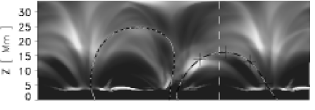
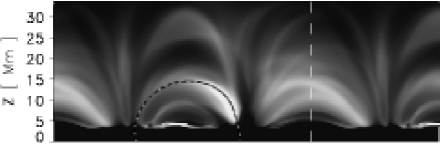
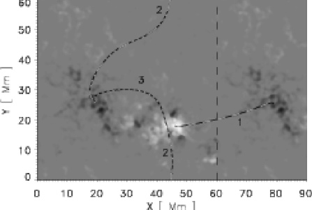
Figure 4.— Emulated TRACE 171 (top) and 195 (middle) with an emulated magnetogram (bottom), showing three loops bright in emission, and 5 points as crosses in the emulated TRACE 171 image which are used to create DEM curves

Figure 5.— Loop 1 with left and right leg in Fig. 4 being to the left and right respectively, for the energy deposition showing heating (solid), radiative cooling (dashed), Spitzer conductivity (dash-dot-dot-dot), convective energy deposition (long dashes) and emission in the TRACE 171 Å filter(dotted) as a function of height

Figure 6.— Gas parameters for loop 1 showing density (solid), gas pressure (dashed), temperature (dotted) and the absolute velocity along the magnetic field (long dashed). For this loop the gas flows down both legs

Figure 3 shows the horizontal width of loops that have a circular-loop cross section at their tops of 0.8 Mm. Loops with a wide variety of maximum heights have been chosen, but there is no obvious dependence of the changes in cross section on the maximum height. It is clear that the loops have significantly smaller cross sections in the photosphere, and that they are non-circular. When moving further up into the transition region, the loops become wider, some having expanded by a factor of ten but generally the expansion is not identical in all directions. That makes the traditional “wine-glass” picture of the magnetic field in the transition region a bad approximation, as Schrijver & Title (2003) have pointed out after modelling of network flux concentrations. There is a tendency for bright TRACE loops to be very asymmetric in the photosphere. It is clear that if these loops are assumed to have circular cross sections at their tops, few (if any) have circular cross sections at a height corresponding to the transition region. Therefore neither cross section nor cross section area are conserved along any of the loops we have followed. In general the foot prints of the loops shown in Fig. 3 are wrinkled and not geometrically simple, and their area cannot be approximated by product of $\Delta X$ and $\Delta Y$. We expect the foot prints to increase in complexity with increasing resolution.

It should be pointed out that the loops followed here are not chosen on the basis of a visible characteristic, but are simply based on choosing random points in the corona, whereafter a set of fieldlines around each point are followed to the photosphere. This means that not all the loops treated here are representative of the observed cross sections of TRACE loops, but lend evidence to the fact that bright loops in general do not have circular cross sections along their whole length. In order to probe the true cross section of loops, the spatial resolution would have to be raised by at least a factor of two, to include velocity gradients produced by flow scales in the photosphere that the resolution here cannot resolve.

Figure 7.— Similar to Fig. 5, here for loop 2

Figure 8.— Similar to Fig. 6, here for loop 2 with many reversals in gas flow direction

3.3. Loop Heating

Loops have in general highly time dependent heating profiles, and the heating is independent in the loop legs. It is thus only possible to define a general heating profile if a large number of loops are used. We obtain an average heating profile that above the transition region decreases exponentially, with a scale length of $\sim 6$ Mm. The height dependence of the heating is highly variable from loop to loop. The scale height behaviour emerges since the heating is proportional to the current squared and because the magnetic field in the corona is close to force free, which makes the current along each fieldline proportional to the magnetic field. In addition to being close to force free, with the property $\vec{J}\propto\vec{B}$, the magnetic field also does not deviate much from a potential field (cf. Sec. 3.1). The overall magnetic field strength thus decreases roughly exponentially with height, with a scale height determined by the distance between the dominating magnetic polarities. In the present periodic model the shortest distance between the two main polarities is roughly half the box size, so at coronal heights the wave number corresponding to the box size $k_{0}$ dominates. Assuming that the magnetic field drops off with height as a potential field we thus obtain

$$Q(z) \propto J^{2}(z)\propto B^{2}(z)\propto\left[\exp{\left(-k_{0}\,z\right)}\right]^{2}$$ (1)

$$\propto e^{-2k_{0}\,z},$$

and so the estimated heating scale height is $s_{H}=1/2k_{0}\sim 5.0$ Mm, consistent with what we actually measure.

In terms of the half loop length $L$ of assumed semicircular loops (cf.  Aschwanden et al., 2001), our estimated heating scale height is

$${s_{H}\over L}={1\over 2k_{0}L}={2\over\pi^{2}}\approx 0.2~{},$$ (2)

where the wave number $k_{0}$ and the half loop length $L$ have been related to the distance between polarities $d$ through $k_{0}=\pi/d$ and $L=\pi d/4$. This is consistent with Aschwanden et al. (2001), who find $s_{H}/L=0.2\pm 0.1$.

3.4. Loop stratification and dynamics

Loops encountered in this model are generally not in equilibrium and a significant fraction of the visible loops identified in the TRACE 171 filter are not aligned with the magnetic field. A possible scenario for such a loop to develop is when one of two connected polarities has a velocity gradient in the direction connecting the two polarities. This implies that one polarity is drawn out along a line perpendicular to the line initially connecting the two polarities, which will create a shear in the field connecting the two. In general the maximum of the shear will not follow a particular fieldline connecting the two polarities. If the shear happens on a short timescale the maximum shear locations will enter the narrow TRACE filters at the same time, showing a bright region that is not connected by a single loop bundle.

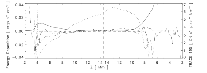
Figure 9.— Similar to Fig. 5, here for loop 3

Figure 10.— Similar to Fig. 6, here for loop 3 with gas flows down both legs from a position just below the loop top in the left leg

Three loops are traced in Fig. 4, where loop 1 and loop 2 are selected for their brightness in the emulated TRACE 171 filter (Fig. 4, top) while loop 3 is selected for its brightness in the emulated TRACE 195 filter (Fig. 4, middle).

Loop 1 can be identified through its whole length in the emulated TRACE 171 filter. It is an example of a steady relatively cold loop and seems to be in a cooling phase. It shows low steady velocities down both of its legs of at most a few tens of $\textrm{km s}^{-1}$. The energy balance and the gas parameters of the loop are shown in Figures 5 and 6, respectively. The heating is growing smoothly towards the photosphere, except for a small bump on the right leg, which could be an impulsive heating event. The convective energy term advects energy from the coronal part of the loop to the denser lower atmosphere, were it is deposited. The Spitzer conductivity shows the characteristic pattern of moving energy from the hot corona and pumping it down into the chromosphere. The radiative cooling is insignificant and shown here without quenching, making it rise sharply when the density increases. This loop is very quiescent except for the bottom of the right leg, which shows large fluctuations in the convective term, due mainly to the large densities, and not so much large velocities. The temperature, density and pressure are very close to constant in most of the corona. There is a slight decrease in temperature, which is large enough to have an effect on the emission in TRACE 171 filter.

Loop 2 is shown in Figures 7 and 8. This loop is an example of a dynamic loop that, in spite of the intermittent velocities present in the loop, is still visible throughout most of its length. This loop has more uneven heating than loop 1. The velocities present in this loop are the effect of the heating and velocities perpendicular to the loop. This loop is much longer than loop 1, even though this is not obvious from Fig. 4 (middle), the top view shows that this loop is much longer than loop 1. Projection effects such as this one are quite common, and lead to confusing and at times misleading conclusions about a particular loop. The special geometry of the loop, with a flat loop top, makes the gradients in velocity in Fig. 8 seem strong because the velocity is plotted against height. In spite of the gradients being smaller than what they seem from Fig. 7, there is still a significant energy reorganisation in this loop. The convective energy term is dominating everything else in the corona produced by velocities of up to 30 km s^-1 in the right leg. The left leg has a distance over which the velocities are on the order of 1 km s^-1. The temperature along the loop is close to constant through the whole corona, while the pressure and density are larger in the left leg, with a noticeable increase in density at the loop top. It is because the loop top is flat that it is possible for this amount of mass to have accumulated at the loop top. It could have happened as the result of powerful heating at both legs, which has now turned off. The evaporated gas would then accumulate at the loop top, and now the loop is cooling down. The low pressure of the right leg is at this point in time not able to support the dense gas at the loop top, which is now falling down the right leg. At the same time there is still material coming up the right leg, and a large amount of convective energy is deposited where the two flows meet. The left leg also has material coming down from the top, but this is slowed down high in the corona, with a corresponding effect on the convective energy term. Below this point gas seems to be free falling due to the very low magnetic heating in the left leg.

Loop 3 is somewhat hotter than loop 1 and 2, and shows up most prominently in TRACE 195. Figures 9 and 10 show that the heating in the right leg is more than a factor of ten higher than in loop 1 and 2, and furthermore is much larger in the right leg, compared to the left. From Fig. 4 one can see that the right leg is rooted in the main polarity, with a magnetic field strength roughly ten times higher than the left leg. Because of the high pressure in the right leg, the transition region is also at different heights in the two legs. In the left leg, the transition region is at a height of 3.5 Mm while in the right leg it is at 7 Mm. As already mentioned the heating is in general dependent on the magnetic field strength and the local height of the transition region. Because of the large differences in magnetic field strength and local height of the transition region, the heating is much stronger in the right leg than in left. In spite of the powerful heating in the right leg, the radiative cooling close to balances the powerful heating. The pressure in the right leg is building, and is now higher than at the top of the loop. Nevertheless, the momentum of the falling gas is still large enough that the increasing pressure gradient is not yet able to break the fall.

4. Time evolution

Loops observed with TRACE and SOHO/EIT can be long lived. Some show life-times much longer than dynamical, cooling and conductive time scales. In following a loop in time we have attempted to follow an emitting plasma-parcel which initially is caught in a flux bundle. The plasma parcel is then followed to the next snap shot, and here the magnetic field is used as a tracer for the rest of the loop. In a 3D simulation like the one discussed here, following a plasma-parcel from one snapshot to the next is theoretically simple. But following a plasma parcel over a long time may require sub-resolution precision, because errors in position accumulate from snapshot to snapshot. Unless the plasma parameters change abruptly there is no way to estimate if an error has been made when following a plasma parcel over long times. In spite of these problems we believe we have managed to follow the time evolution of loop 1 with good precision for more than 20 minutes. The emission in TRACE 171 is shown in Fig. 11, in units of DN s^-1 pixel^-1 Mm^-1 (making the actual photon count rate depend on the thickness of the loop as well as on the background and foreground). One resolution element, emitting at the level of most of the upper part of the loop, makes up  10 % of the typical level of emission from a loop seen in Fig. 4. The loops in this simulation are in general thicker than in the solar corona, because of the limited resolution in the photosphere, which sets the minimum driving scale. After the expansion of the magnetic field through the chromosphere and transition region, this makes the loops in the simulated corona thicker than on the Sun. In this simulation, loops generally are on the order of 6-8 grid cells thick or 3̃ Mm. In spite of the very dynamic nature of the loop 1, it manages to stay bright along most of its length during the whole 20 min time period. The dark left leg of loop 1 is caused by a too high temperature, moving that leg outside the temperature response function of the TRACE 171 filter. The reason that the leg is still apparent in Fig. 4 (top) is the large amount of other loops originating in the same area. Fig. 11 clearly shows that it is possible to have long lived, non static loops in a corona produced by a highly time dependent DC heating mechanism.

5. Differential Emission Measure

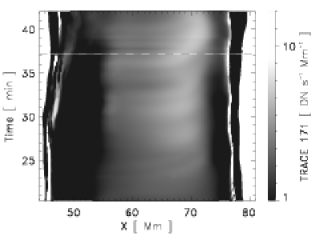
Figure 11.— Emission in the TRACE 171 filter as function of time for loop 1. The dashed line shows the time of Fig. 4

DEM can be constructed from observations of a number of lines, essentially giving a measure for the amount of emitting gas at a certain temperature. DEM can also be constructed by comparing emission in a number of narrow filters, such as the ones used by EIT and TRACE. Constructing DEM curves on the basis of narrow band observations is however an ill posed problem, and whether any trustworthy information can be gained from such exercises has been the subject of intense discussion(Schmelz et al., 2001; Martens et al., 2002; Aschwanden, 2002). Creating DEM curves from a 3D simulation is more straight forward. The DEM can be defined as

$$\textrm{DEM}=n_{e}\frac{dh}{dT}\,,$$ (3)

which, when defining a volume emission measure ($\textrm{EM}_{V}$) as

$$\textrm{EM}_{V}(T)=\int_{V}n_{e}^{2}dV\,,$$ (4)

makes it possible to find the DEM from the simulation simply as

$$\textrm{DEM}=\frac{\textrm{EM}_{V}}{A\,\Delta T}$$ (5)

where $A$ is the area of a grid cell. When constructing DEM curves $\Delta T$ is often not constant, but instead constant logarithmic intervals are used. In this case we use temperature intervals of $d\textrm{Log}_{10}T=0.1$. The intervals are furthermore over sampled in the sense that intervals overlap in order to be able to construct reasonably smooth curves.

Figure 12.— DEM curves for the five points along loop 1 shown in Fig. 4. The points are numbered from left to right with numbers 1 to 5. Curves 2-5 are shifted up by 1-4 orders of magnitude respectively

DEM curves for 5 selected points along loop 1, shown as crosses in Fig. 4 (top), are shown in Fig. 12. It is very difficult to identify loop 1 from these curves, and it is also clear that especially for points 2 and 3, the typical temperature visible in TRACE 171 is not the temperature where most of the gas is. Point 5 shows especially many isolated bumps, while point 3, even though it seems to be in the middle of a bright loop, show a clear bump at low temperatures. These DEM curves are representative of most of the ones we have produced and one can only seldomly find clear signatures of loops, because of the ”pollution” of loops seen in images like Fig. 4 (top). In spite of these problems, it seems that in this model, loops typically have a DEM of $10^{21}-10^{22}\,\textrm{cm}^{-5}\,\textrm{K}^{-1}$ near 1 MK. This level of emission measure is also what for instance Schmelz et al. (2003) finds. In the same work (Schmelz et al., 2003) argue that because the maximum for their DEM curves along the loop is not at the same temperature one has to be very careful in employing this method. We agree on this point, but not on the conclusion that the non constant maximum of the DEM curve is evidence for a temperature gradient along the loop. The conclusion would hold true if the loop were perfectly isolated in temperature. This is very seldomly the case. By visual inspection, loop 1 seems to be reasonably isolated in Fig. 4 (top), but we have seen that at the left leg this is not so, even though along some of its length it is true. Figure 13 shows the temperature of the gas and the contribution to the emission in TRACE 171 along the projected axis in Fig. 4 (top) of point 4. It is also clear that the sharp peak in emission is located in a temperature dip, and that even though there are quite a few areas at a temperature which should show up in the TRACE 171 filter, these are not important, because the density is too low. The DEM is able to show the range of temperatures involved but in spite of the sharp peak in emission in the TRACE 171 filter, it is not clearly noticeable in the DEM curve. It therefore seems that a simplistic approach to DEM curves is a problematic way of trying to identify loops.

Figure 13.— Emission contribution (solid) and temperature (dashed) along the projected axis at point 4 of loop 1 shown in Fig. 4 (top)

The problem would become more severe when also the resolution is worse than the typical width of a loop, since this would introduce not only contamination along the line of sight, but also in the 2D viewing plane.

6. Discussion and Conclusions

The three loops discussed here are representative of a large number of loops we have examined and illustrate that there are no static loops. Loops are continuously changing, with large differences in heating, cooling and cross sections. It is therefore futile to fit scaling relations to individual loops, since the scaling properties will change with time and between loops, making any scaling relations inexact. We have seen examples of loops in the emulated TRACE pass bands that do not follow fieldlines, because the field is sheared and heating is localised in thin structures across fieldlines. The high thermal conductivity adjusts the temperature gradient until conduction balances the heating rate, and makes the effect hard to observe except when projection effects add up contributions from the slightly brighter sheared heating region.

When looking at large ensembles of loops in an active region the heating scales roughly with the magnetic field strength squared and decreases exponentially from the local height of the transition region. The scale height is essentially proportional to the mean separation of the main polarities in the active region.

Velocities in loops are assumed to be along fieldlines, and that is what we find in the region just above the transition region. Above roughly 10 Mm the velocities along the loops relative to the total velocity amplitudes are no longer close to unity, but span the whole interval between zero and one. The velocity amplitudes are on average a few tens of km $\textrm{s}^{-1}$, but velocities as high as 400 km $\textrm{s}^{-1}$ are present.

Density and pressure are less extreme in these loops than what has been reported for long loops by Winebarger et al. (2003), and are here only a few times denser than the surroundings. It is, however, clear that the density is approximately constant along loops. The loops therefore show no decrease in emission measure with height. This simulation only spans 37 Mm in height, slightly less than a pressure scale height for a 1 million degree gas, and therefore we cannot say if higher loops would show a decrease in density with height but since the heating scale height also tends to increase with active region size, we expect loops to be able to keep approximately constant density, or at least have densities decreasing slower with height than for an atmosphere in hydrostatic equilibrium.

Both heating and plasma flows are time dependent for loop 1, even though it has an almost constant emission throughout the time span we followed it. The coronal loops analysed here may be assumed to be generic, but are most likely not representative of many of the loops observed by TRACE and analysed in detail elsewhere since the latter are biased towards being bright, isolated and long. The DEM curves measured for the bright TRACE 171 loop do not easily reveal a loop, and as already concluded by Schmelz et al. (2003), differential emission measures must be treated carefully if they are to be used.

The magnetic field in this work is only disturbed slightly from a potential field, so large scale helicity is not present. Large scale helicity is often present in observed active regions on the Sun and may be caused by large scale velocity fields, or may exist already in the flux emergence phase. Including disturbances able to create systematic helicity would introduce unknown or arbitrary variables in contrast to the ab initio approach of this work, but we do expect that if a number of short loops in quiescent active regions are observed in the TRACE or EIT 171 band similar loops as modelled here would be present.

Analysis of this simulation indicates that often-made assumptions, such as those of hydrostatic equilibrium, a time independent and symmetric heating function, and constant cross sections along loops are highly questionable and cannot provide a basis for simplified models of loops.

References

- Aschwanden et al. (2001) Aschwanden, M., Shrijver, C., & Alexander, D. 2001, ApJ, 550, 475
- Aschwanden (2002) Aschwanden, M. J. 2002, ApJ, 580, L79
- Carlsson & Stein (2002) Carlsson, M. & Stein, R. F. 2002, ApJ, 572, 626
- Del Zanna & Mason (2003) Del Zanna, G. & Mason, H. E. 2003, A&A, 406, 1089
- Fontenla et al. (1993) Fontenla, J. M., Avrett, E. H., & Loeser, R. 1993, ApJ, 406, 319
- Gudiksen & Nordlund (2004) Gudiksen, B. & Nordlund, Å. 2004, ApJ, submitted
- Martens et al. (2002) Martens, P. C. H., Cirtain, J. W., & Schmelz, J. T. 2002, ApJ, 577, L115
- Peter et al. (2004) Peter, H., Gudiksen, B. V., & Nordlund, Å. 2004, A&A, In Press
- Priest & Démoulin (1995) Priest, E. R. & Démoulin, P. 1995, J. Geophys. Res., 100, 23443
- Rosner et al. (1978) Rosner, R., Tucker, W. H., & Vaiana, G. S. 1978, ApJ, 220, 643
- Schmelz et al. (2003) Schmelz, J. T., Beene, J. E., Nasraoui, K., et al. 2003, ApJ, 599, 604
- Schmelz et al. (2001) Schmelz, J. T., Scopes, J. E., Cirtain, J. W., Winter, H. D., & Allen, J. D. 2001, ApJ, 556, 896
- Schrijver & Title (2003) Schrijver, C. J. & Title, A. M. 2003, ApJ, 597, L165
- Serio et al. (1981) Serio, S., Peres, G., Vaiana, G. S., Golub, L., & Rosner, R. 1981, ApJ, 243, 288
- Solanki et al. (2003) Solanki, S., Lagg, A., Woch, J., Krupp, N., & Collados, M. 2003, Nature, 423, 692
- Testa et al. (2002) Testa, P., Peres, G., Reale, F., & Orlando, S. 2002, ApJ, 580, 1159
- Warren et al. (2003) Warren, H. P., Winebarger, A. R., & Mariska, J. T. 2003, ApJ, 593, 1174
- Winebarger et al. (2003) Winebarger, A. R., Warren, H. P., & Mariska, J. T. 2003, ApJ, 587, 439