Late time behavior of cosmological perturbations in a single brane model

Abstract

We present solutions for the late time evolution of cosmological tensor and scalar perturbations in a single-Randall-Sundrum brane world model. Assuming that the bulk is anti-de Sitter spacetime, the solutions for cosmological perturbations are derived by summing mode functions in Poincaré coordinate. The junction conditions imposed at the moving brane are solved numerically. The recovery of 4-dimensional Einstein gravity at late times is shown by solving the 5-dimensional perturbations throughout the infinite bulk. We also comment on several possibilities for having deviations from 4-dimensional Einstein gravity.

1 Introduction

Since the possibility that we are living on a brane in a higher dimensional spacetime was proposed, much effort has been devoted to investigating the cosmology of brane worlds [1]. A model proposed by Randall and Sundrum (RS) provided a very simple and interesting playground in which to investigate brane world cosmology [2]. In their model, our world is realized on a four-dimensional brane in five-dimensional spacetime. The remarkable feature of this model is that the size of extra dimension could be infinite. A homogeneous and isotropic cosmological solution was found [3]-[6] and then the theory of cosmological perturbation has been extensively investigated [7]-[37] (see [38] for a review). The study of cosmological perturbation is very important because it can provide a means for testing brane world models using forthcoming precise cosmological observations. However, it turns out that the analysis of cosmological perturbation in brane worlds is extremely difficult. Although a large number of papers has been published on this subject, there are rather few quantitative predications. This is because the evolution of perturbations on the brane is inevitably coupled to the perturbations in the five-dimensional bulk. Thus we need to solve very complicated coupled partial differential equations with complicated boundary conditions that arise from the brane.

Although some progress has been made in a model where a higher dimensional spacetime is bounded by two branes [39] [40], there is still no quantitative prediction of the evolution of perturbations in a single-brane model. The crucial difficulty of the single brane model is that the bulk spacetime extends to an infinity. A useful method for tackling this problem was proposed in Ref.[12], [23] (see also [16], [19] and [36]). One point is that the background 5-dimensional spacetime is just the anti de Sitter (AdS) spacetime (or AdS-Schwarzshild spacetime) in the RS model. Thus we can easily find general solutions for the perturbations throughout the bulk. A difficulty arises from the existence of the brane. We need to select a particular solution that correctly satisfies the boundary conditions at the brane. In this paper, we present a solution for this problem using a numerical method. Then the late time behavior of the perturbations is derived by solving the 5-dimensional perturbations throughout the infinite bulk. In this paper the bulk spacetime is assumed to be AdS spacetime without black holes and we only consider the late time behavior of the perturbations. The generalization of the analysis will be discussed in the conclusion section.

The structure of the paper is as follows. In Section 2, we describe the set-up of our model. In section 3, the solution for background spacetime is derived. In section 4, an evolution of tensor perturbation is considered. We describe the numerical method used to solve the moving boundary conditions here. In section 5, a more complicated evolution of scalar perturbations is derived. In section 6, we try to interpret our result using the gradient expansion method. Conclusions and a discussion of the generalization of our work are given in Section 7.

2 The setup

We consider the 5D action of the RS model:

$$S = \frac{1}{2\kappa^{2}}\int d^{5}x\sqrt{-g}\left({\cal R}^{5}+12\mu^{2}\right)-\lambda\int d^{4}x\sqrt{-g_{brane}}$$ (1)

$$+\int d^{4}x\sqrt{-g_{brane}}{\cal L}_{matter},$$

where ${\cal R}^{5}$ is the 5D Ricci scalar, $\mu$ is the curvature scale of the AdS spacetime and $\kappa^{2}=8\pi G_{5}$ where $G_{5}$ is the Newton’s constant in the 5D spacetime. The brane has tension $\lambda$ and the induced metric on the brane is denoted as $g_{brane}$. The tension $\lambda$ of the brane is taken as $\kappa^{2}\lambda=6\mu$ to ensure that the brane becomes Minkowski spacetime if there is no matter on the brane. Matter is confined to the 4D brane world and is described by the Lagrangian ${\cal L}_{matter}$. We will assume $Z_{2}$ symmetry across the brane. On the brane, the metric is given by

$$ds^{2}_{brane}=-dt^{2}+a_{o}(t)^{2}\delta_{ij}dx^{i}dx^{j}.$$ (2)

We will decompose the perturbations into scalar, vector and tensor ones defined with respect to 3-space $\delta_{ij}$ and only consider tensors and scalars in this paper. The energy momentum tensor of the matter confined to the brane is given by $T^{\mu}_{\nu}=T^{\mu}_{B\>\nu}+\delta T^{\mu}_{\nu}$;

$$T^{\mu}_{B\>\nu}=diag(-\rho,p,p,p),\quad p=w\rho,$$ (3)

$$\delta T^{\mu}_{\nu}=\left(\begin{array}[]{cc}-\delta\rho&\delta q_{,i}\\ a_{o}^{-2}\delta q_{,i}&\delta p\>\delta_{ij}\\ \end{array}\right).$$ (4)

Here the matter anisotropic stress is neglected for simplicity.

3 Background spacetime

In this section, we briefly consider the background spacetime. In this paper, we only consider the maximally symmetric bulk spacetime, that is, we assume that the bulk spacetime is given by Anti de Sitter (AdS) spacetime without a black hole mass. The simplest coordinate system for describing AdS spacetime is given by the Poicare coordinate:

$$ds^{2}=\left(\frac{1}{\mu z}\right)^{2}(dz^{2}+\eta_{\mu\nu}dx^{\mu}dx^{\nu}).$$ (5)

Our brane is moving in this coordinate system. The motion of the brane is determined by imposing the junction condition. The brane motion is described by [4]

$$z=\frac{1}{\mu a_{o}(t)},\tau=T(t),$$ (6)

where

$$H^{2} = \left(\frac{\dot{a_{o}}}{a_{o}}\right)^{2}=\frac{\kappa^{2}\mu\rho}{3}+\frac{\kappa^{4}\rho^{2}}{36},$$

$$\dot{T} = \frac{1}{a_{o}}\sqrt{1+\left(\frac{H}{\mu}\right)^{2}},$$ (7)

where $t$ is the cosmic time on the brane and a dot denotes the derivative with respect to $t$. The expansion of the universe can be understood as the motion of the brane through the bulk.

Of course, the statement that our brane is moving is a coordinate dependent statement. It is possible to choose coordinates where the position of the brane is fixed. The Gaussian-Normal (GN) coordinate is such a coordinate. The metric is given by [3]

$$ds^{2}=dy^{2}-n(y,t)^{2}dt^{2}+a(y,t)^{2}\delta_{ij}dx^{i}dx^{j},$$ (8)

where

$$a(y,t) = a_{o}(t)\left[\cosh\mu y-\left(1+\frac{\kappa^{2}\rho}{6\mu}\right)\sinh\mu y\right],$$

$$n(y,t) = \cosh\mu y-\left(1-\frac{\kappa^{2}\rho}{6\mu}(2+3w)\right)\sinh\mu y.$$ (9)

The brane is located at $y=0$. This coordinate is convenient for imposing the junction conditions because the position of the brane is fixed. The junction conditions in the background spacetime are given by

$$\left(\frac{a^{\prime}}{a}\right)_{b} = -\mu\left(1+\frac{\kappa^{2}\rho}{6\mu}\right),$$

$$\left(\frac{n^{\prime}}{n}\right)_{b} = -\mu\left(1-\frac{\kappa^{2}\rho}{6\mu}(2+3w)\right),$$ (10)

where the subscript b is used to denote bulk quantities evaluated at the brane. Using the Freidmann equation, the former equation can be written as

$$\left(\frac{a^{\prime}}{a}\right)_{b}=-\mu\sqrt{1+\left(\frac{H}{\mu}\right)^{2}}.$$ (11)

Note that there is a coordinate singularity in this coordinate $y_{c}$ at the finite distance from the brane where $a(y_{c},t)=0$. This hypersurface corresponds to the past Cauchy horizon of the AdS spacetime. Thus, this coordinate is not suitable for discussing the global structure of the solution in the bulk. However, in order to impose the junction conditions, we need only know the geometry of the bulk near the brane. Thus we will solve for the bulk perturbations in Poincaré coordinate and move to the GN coordinate when we impose the boundary conditions. In order to do so, we need to rewrite the junction conditions in the GN coordinate as conditions in Poincaré coordinate. The coordinate transformation between the two coordinate systems has been investigated in Ref.[6]. The transformation is very complicated, but we only need the formula relating the derivative with respect to the GN coordinate to the derivative with respect to Poincaré coordinate on the brane. This is given by the following formulae;

$$\left(\frac{\partial\tau}{\partial y}\right)_{b} = -\frac{1}{a_{o}}\frac{H}{\mu},\quad\left(\frac{\partial z}{\partial y}\right)_{b}=\frac{1}{a_{o}}\sqrt{1+\left(\frac{H}{\mu}\right)^{2}},$$

$$\left(\frac{\partial z}{\partial t}\right)_{b} = -\frac{1}{a_{o}}\frac{H}{\mu},\quad\left(\frac{\partial\tau}{\partial t}\right)_{b}=\frac{1}{a_{o}}\sqrt{1+\left(\frac{H}{\mu}\right)^{2}}.$$ (12)

4 Tensor perturbation

Let us begin with the tensor perturbation:

$$ds^{2}=\left(\frac{1}{\mu z}\right)^{2}\left(dz^{2}-d\tau^{2}+(\delta_{ij}+h_{ij})dx^{i}dx^{j}\right).$$ (13)

We expand $h_{ij}$ as

$$h_{ij}=\int\frac{d^{3}k}{(2\pi)^{3}}h(z,\tau)e_{ij}e^{ikx},$$ (14)

where $e_{ij}$ is the polarisation tensor. The evolution equation is simply given by

$$\frac{d^{2}h}{dz^{2}}-\frac{3}{z}\frac{dh}{dz}-\frac{d^{2}h}{d\tau^{2}}-k^{2}h=0.$$ (15)

It is easy to find a solution

$$h(z,\tau)=\int dmh(m)z^{2}Z_{2}(mz)\left(e^{i\omega\tau}+c(m)e^{-i\omega\tau}\right),$$ (16)

where

$$Z_{2}(mz)=H_{2}^{(2)}(mz)+b(m)H_{2}^{(1)}(mz),$$ (17)

and $\omega^{2}=m^{2}+k^{2}$. Here $H^{(1)}$ and $H^{(2)}$ are Hankel functions of the first kind and the second kind respectively and $h(m),b(m)$ and $c(m)$ are arbitrary coefficients. This is a general solution for tensor perturbations in the AdS bulk. Our spacetime is bounded by the brane. Thus we should impose a boundary condition via a junction condition. In the GN coordinate, the junction condition is simply given by

$$\left[\frac{\partial h}{\partial y}\right]_{y=0}=0.$$ (18)

Using the formulation equations (12), we can rewrite this condition in terms of the Poincaré coordinate

$$\left[\frac{\partial h}{\partial z}-\frac{H}{\mu}\left(1+\left(\frac{H}{\mu}\right)^{2}\right)^{-1/2}\frac{\partial h}{\partial\tau}\right]_{z=1/\mu a_{o}(t),\tau=T(t)}=0.$$ (19)

Let us impose the boundary condition Eq.(19) on a general solution given by

$$h(z,\tau)=\int dmh(m)m^{2}z^{2}Z_{2}(mz)e^{i\omega\tau}.$$ (20)

The boundary condition of equation (19) gives

$$\int dmh(m)\left[\frac{m^{3}}{\mu^{2}a_{o}^{2}}Z_{1}\left(\frac{m}{\mu a_{o}}\right)-\frac{H}{\mu}\left(1+\left(\frac{H}{\mu}\right)^{2}\right)^{-1/2}\frac{i\omega m^{2}}{\mu^{2}a_{o}^{2}}Z_{2}\left(\frac{m}{\mu a_{o}}\right)\right]e^{i\omega T}$$

$$=0.$$ (21)

The problem is finding the solution for $h(m)$ that satisfies this boundary condition. In order to find the solution, we need a numerical method.

As suggested by recent numerical works [32], [35], we expect the behavior of the perturbation to be well described by a standard 4D Einstein gravity at low energies $H/\mu\ll 1$. We can argue on the recovery of the 4D solution as follows. At late times, it is natural to assume that the Kaluza Klein (KK) mass is small compared with the bulk curvature scale because the Hubble scale of the brane universe is much smaller than the bulk curvature scale $H/\mu\ll 1$. So we assume

$$\frac{m}{\mu a_{o}}\equiv\epsilon\ll 1.$$ (22)

Then expanding in terms of $\epsilon$ by using the asymptotic behavior of Hankel functions with small arguments,

$$H^{(1)}_{\nu}(z)\sim-i\frac{(\nu-1)!}{\pi}\left(\frac{2}{z}\right)^{\nu},\quad H^{(2)}_{\nu}(z)\sim i\frac{(\nu-1)!}{\pi}\left(\frac{2}{z}\right)^{\nu},\quad$$ (23)

the general solution of equation (20) on the brane becomes

$$h_{b}(t)\sim\int dmh(m)e^{i\omega\eta},$$ (24)

where we neglected the numerical factor and used $T(t)=\eta$ at late times where $\eta$ is the conformal time. On the other hand, the boundary condition of equation (21) becomes

$$0=\int dm\left(\frac{m^{2}}{a_{o}}-2i\omega H+{\cal O}\left(\epsilon^{4},\epsilon^{4}\log\epsilon\right)\right)h(m)e^{i\omega\eta}.$$ (25)

Then on rewriting $m^{2}=k^{2}+\omega^{2}$ and $\omega$ in terms of the derivative with respect to conformal time, this condition can be written as

$$\left(-\frac{d^{2}}{d\eta^{2}}-2\frac{1}{a_{o}}\frac{da_{o}}{d\eta}\frac{d}{d\eta}-k^{2}\right)h_{b}=0.$$ (26)

This is noting but the evolution equation obtained in 4D Einstein gravity for the tensor perturbation. It implies that, at late times $H/\mu\ll 1$, the boundary condition selects a particular solution that obeys the 4D evolution equation on the brane. It should be noted that the excitation of KK modes in Poincaré modes is necessary in order to satisfy the boundary condition because zero-mode solution is just $e^{ik\eta}$. The movement of the brane excites KK modes. They give the damping of zero-mode and give the friction term in Eq.(26).

However, the above argument assumes that the junction condition (21) can be satisfied by the KK modes with the condition (22). It only ensures that once there is a solution for $h(m)$ that satisfies the condition (22), the 4D evolution equation is recovered. We should check that there exists a solution for the junction condition (21) that satisfies the condition (22). For this purpose, the spectrum of the KK mass should be determined by imposing the junction condition at the brane (21) as well as the initial conditions and the boundary condition in the bulk.

Let us try to find solutions for $b(m),c(m)$ and $h(m)$ numerically. We first specify the boundary condition at the AdS past Cauchy horizon, which corresponds to the infinity $z\to\infty$. The most natural assumption is that the wave is outgoing, so that there is no incoming radiation. We demand

$$h\propto\int dmz^{3/2}e^{im(z-\tau)},$$ (27)

for $z\to\infty$ and $k\to 0$. This condition gives $b(m)=c(m)=0$. Then we impose the boundary condition of equation (21) at the brane. This condition is formally written as

$$\int dmh(m){\cal B}(m,t)=0.$$ (28)

We numerically find solutions for $h(m)$ that satisfy this boundary condition approximately. We first discretize time $t$ and a KK mass $m$. Then we end up a matrix equation. A problem is finding eigenvectors with a null eigenvalue. In principle there could be an infinite number of solutions for $h(m)$. However we expect that an excited KK mass is small at low energies $H/\mu\ll 1$ as long as we consider an initial condition that does not contain a significant excitation of KK modes. Thus we introduce a cut-off for $m$. Then we can find finite numbers of approximate solutions for $h(m)$. In addition, we should determine the initial condition. Here we adopt an ad hoc initial condition that the perturbation is constant with respect to $t$ on the brane at super-horizon scales. This can be achieved by mixing the real part and the imaginary part of $h$ appropriately. Then we obtain a real solution for $h$. In appendix C, the accuracy of the numerical calculation is shown.

Figure 1 shows two solutions for $h(m)$ from numerical results. We take $H/\mu=0.0001$ at the horizon crossing as an example. As expected we need the KK modes to satisfy the boundary condition but the excited KK mass is small compared with $\mu$. If we sum the mode functions with the weight $h(m)$, we recover the 4D behavior of the perturbation on the brane (Figure 2).

We would like to make a comment on the cut-off of the KK modes introduced in the numerical calculations. As is seen from the Figure 1, the solution obtained for $h(m)$ is localized around $m/\mu<0.2$ which is well below the artificial cut-off at $m/\mu=1.2$. We have confirmed the existence of the solution for $h(m)$ that is localized around $m/\mu<0.2$ even if we increase the cut-off up to $m/\mu=2.4$. Thus the existence of the solution with $m/\mu a_{o}<<1$ does not depend on the artificial cut-off of the KK mass. On the other hand, the introduction of the cut-off certainly kills the solutions that have large $m/\mu a_{o}$. Thus our analysis is limited to the solutions with the KK mass below the cut-off.

Figure 1: Solutions for $h(m)$. The vertical line is $m/\mu$. We take $H/\mu=0.0001$ at the horizon crossing and the universe is assumed to be radiation dominated. The cut-off is introduced at $m/\mu=1.2$.

The different solutions for $h(m)$ correspond to different initial profiles in the bulk (Figure 3). In this sense, we have not solved the problem yet. In order to find the solution that corresponds to a given initial profile, we again sum solutions with different $h(m)$. Fortunately, we find that the different solutions $h(m)$ give the same solution on the brane. This indicates that the recovery of the 4D behavior does not depend on the choice of the initial profile, as long as the initial profile does not contain large KK masses.

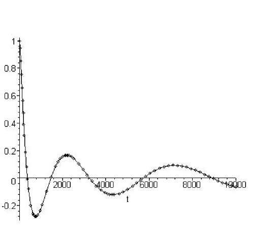
Figure 2: Behavior of the solution $h_{b}$ on the brane. The horizontal axis is the cosmic time. The solid line is the prediction of 4D cosmology with the same initial condition. The points represent the solutions in the brane world obtained by summing the Poincaré mode functions with the weight $h(m)$. All solution for $h(m)$ found in numerical calculations reproduces the 4D behavior of the perturbation.

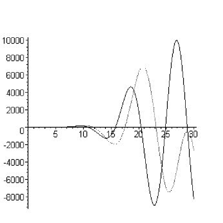
Figure 3: The initial profile of the solution $h(t_{i},z)$ in the bulk. The horizontal axis is $\mu z$. The solid line corresponds to the solution derived from $h(m)$ in the left panel of Figure 1 and the dotted line corresponds to that in the right panel.

If we include the high energy corrections ${\cal O}(H/\mu)$, the behavior of the perturbation significantly deviates from 4D one. The difficulty of the high energy corrections is that the corrections depend on the choice of the initial conditions. Unlike the late time evolution, the different solutions for $h(m)$ give different evolutions on the brane. Thus, unless we perform the summation of the solutions with different $h(m)$ we cannot get the final answer. As we mentioned, the different solutions for $h(m)$ correspond to different initial profiles. Thus this indicates the sensitivity of the solution to the choice of initial conditions. A detailed study of the high energy correction is beyond the scope of this paper and it will be reported in a separate publication [41].

5 Scalar perturbation

Now let us consider the scalar perturbation. There are several ways to calculate the scalar perturbation in AdS spacetime. Here we describe an approach based on a master variable. Using the generalized 5D longitudinal gauge, the perturbed spacetime is given by [11]

$$ds^{2} = b(y,t)^{2}(1+2A_{yy})dy^{2}+n(y,t)A_{y}dydt-n(y,t)^{2}(1+2A^{2})dt^{2}$$ (29)

$$+a(y,t)^{2}(1+2{\cal R})\delta_{ij}dx^{i}dx^{j}.$$

It was shown that the solution for metric perturbations can be derived from a master variable $\Omega$ [7] [8] [22] [27];

$$A = -\frac{1}{6a}\left\{\frac{1}{b^{2}}\left[2\Omega^{\prime\prime}-\left(2\frac{b^{\prime}}{b}+\frac{n^{\prime}}{n}\right)\Omega^{\prime}\right]+\frac{1}{n^{2}}\left[\ddot{\Omega}-\left(2\frac{\dot{b}}{b}+\frac{\dot{n}}{n}\right)\dot{\Omega}\right]-\mu^{2}\Omega\right\}\,,$$

$$A_{y} = \frac{1}{na}\left(\dot{\Omega}^{\prime}-\frac{n^{\prime}}{n}\dot{\Omega}-\frac{\dot{b}}{b}\Omega^{\prime}\right)\,,$$

$$A_{yy} = \frac{1}{6a}\left\{\frac{1}{b^{2}}\left[\Omega^{\prime\prime}-\left(2\frac{n^{\prime}}{n}+\frac{b^{\prime}}{b}\right)\Omega^{\prime}\right]+\frac{1}{n^{2}}\left[2\ddot{\Omega}-\left(2\frac{\dot{n}}{n}+\frac{\dot{b}}{b}\right)\dot{\Omega}\right]+\mu^{2}\Omega\right\}\,,$$

$${\cal R} = \frac{1}{6a}\left\{\frac{1}{b^{2}}\left[\Omega^{\prime\prime}+\left(\frac{n^{\prime}}{n}-\frac{b^{\prime}}{b}\right)\Omega^{\prime}\right]+\frac{1}{n^{2}}\left[-\ddot{\Omega}+\left(\frac{\dot{n}}{n}-\frac{\dot{b}}{b}\right)\dot{\Omega}\right]-2\mu^{2}\Omega\right\}\,,$$ (30)

as long as the master variable $\Omega$ in the bulk satisfies a wave equation given by

$$-\left({b\over na^{3}}\dot{\Omega}\right)^{\cdot}+\left({n\over ba^{3}}\Omega^{\prime}\right)^{\prime}+\left(\mu^{2}+{\nabla^{2}\over a^{2}}\right){nb\over a^{3}}\Omega=0\,.$$ (31)

In Poincaré coordinate, the master equation is given by

$$\frac{d^{2}\Omega}{dz^{2}}+\frac{3}{z}\frac{d\Omega}{dz}+\frac{\mu^{2}}{z^{2}}\Omega-\frac{d^{2}\Omega}{d\tau^{2}}+\nabla^{2}\Omega=0$$ (32)

The solution is easily found as [8]

$$\Omega=-\frac{2}{z}\mu^{-3}\int\frac{d^{3}k}{(2\pi)^{3}}\int dmS(m)Z_{0}(mz)e^{-i\omega\tau}e^{ikx}.$$ (33)

A factor $-2$ was added just for later convenience.

The junction conditions are much more complicated. In order to impose the junction conditions, we move to the GN coordinate. The junction conditions have been found already in literatures (see [8] and [27]), but, for completeness, we briefly discuss the way to impose junction conditions on a master variable in Appendix A. The junction conditions give the expressions for matter perturbations on the brane in terms of a master variable;

$$a_{o}\kappa^{2}\delta\rho = -\frac{k^{2}}{a^{2}}\left(\Omega^{\prime}-\frac{a^{\prime}}{a}\Omega\right)-3\frac{\dot{a}}{a}\left(\dot{\Omega}^{\prime}-\frac{n^{\prime}}{n}\dot{\Omega}\right),$$

$$a_{o}\kappa^{2}\delta q = -\left(\dot{\Omega}^{\prime}-\frac{n^{\prime}}{n}\dot{\Omega}\right),$$

$$a_{o}\kappa^{2}\delta p = \ddot{\Omega}^{\prime}-\frac{a^{\prime}}{a}\ddot{\Omega}+2\frac{\dot{a}}{a}\left(\dot{\Omega}^{\prime}-\frac{n^{\prime}}{n}\dot{\Omega}\right)+\left\{4\frac{\dot{a}}{a}\left(\frac{a^{\prime}}{a}-\frac{n^{\prime}}{n}\right)+2\left(\frac{\dot{a}}{a}\right)^{\prime}-\left(\frac{\dot{n}}{{n}}\right)^{\prime}\right\}\dot{\Omega}$$

$$- \frac{2}{3}\left(\frac{a^{\prime}}{a}-\frac{n^{\prime}}{n}\right)\frac{k^{2}}{a^{2}}\Omega+\mu^{2}\left(\frac{a^{\prime}}{a}-\frac{n^{\prime}}{n}\right)\Omega-\left(\frac{a^{\prime}}{a}-\frac{n^{\prime}}{n}\right)\left(2\frac{a^{\prime}}{a}-\frac{n^{\prime}}{n}\right)\Omega^{\prime},$$

where the prime denotes $\partial_{y}$ and dot denotes $\partial_{t}$ in the GN coordinate and the right hand side of the equation should be evaluated at the brane. Imposing the equation of state $\delta p=c_{s}^{2}\delta\rho$, we get the boundary condition for $\Omega$.

It is more convenient to rewrite these equations into the follwoing form using the expressions for metric perturbations in terms of a master variable equations (30) as

$$-\frac{1}{2}\kappa^{2}{\cal H}\delta\rho = 3H(\dot{{\cal R}}-HA)+\frac{k^{2}}{a_{o}^{2}}{\cal R}-\frac{1}{2}\kappa_{4}^{2}\delta\rho_{{\cal E}},$$

$$-\frac{1}{2}\kappa^{2}{\cal H}\delta p = -\ddot{{\cal R}}-H\left(3-\frac{\dot{H}}{{\cal H}^{2}}\right)\dot{{\cal R}}+H\dot{A}+\left(2\dot{H}+3H^{2}-\frac{H^{2}\dot{H}}{{\cal H}^{2}}\right)A$$

$$-\frac{1}{3}\frac{k^{2}}{a_{o}^{2}}A-\frac{1}{3}\left(1-\frac{\dot{H}}{{\cal H}^{2}}\right)\frac{k^{2}}{a_{o}^{2}}{\cal R}-\frac{1}{6}\left(1+\frac{\dot{H}}{{\cal H}^{2}}\right)\kappa_{4}\delta\rho_{{\cal E}},$$

$$-\frac{1}{2}\kappa^{2}{\cal H}\delta q = \dot{{\cal R}}-HA-\frac{1}{2}\kappa_{4}^{2}\delta q_{{\cal E}},$$

$$0 = \frac{1}{a_{o}^{2}}(A+{\cal R})+\kappa_{4}^{2}\delta\pi_{{\cal E}},$$ (35)

where we defined

$${\cal H}\equiv\left(\frac{a^{\prime}}{a}\right)_{b}=-\mu\sqrt{1+\left(\frac{H}{\mu}\right)^{2}},\quad\kappa_{4}^{2}=\kappa^{2}\mu,$$ (36)

and

$$\kappa_{4}^{2}\delta\rho_{{\cal E}} = \frac{k^{4}\Omega}{3a_{o}^{5}},$$

$$\kappa_{4}^{2}\delta q_{{\cal E}} = \frac{k^{2}}{3a_{o}^{3}}\left(\frac{\dot{a_{o}}}{a_{o}}\Omega-\dot{\Omega}\right),$$

$$\kappa_{4}^{2}\delta\pi_{{\cal E}} = \frac{1}{6a_{o}^{3}}\left(3\ddot{\Omega}-3H\dot{\Omega}+\frac{k^{2}}{a_{o}^{2}}\Omega-3\left(\frac{n^{\prime}}{n}-\frac{a^{\prime}}{a}\right)_{b}\Omega^{\prime}\right).$$ (37)

These equations can be derived from the projected Einstein equation on the brane [42];

$$G_{\mu\nu}+{\cal E}_{\mu\nu}=\kappa_{4}^{2}T_{\mu\nu}+\kappa^{4}\Pi_{\mu\nu},$$ (38)

where

$$\Pi_{\mu\nu}=-\frac{1}{4}T_{\mu\alpha}T_{\nu}^{\alpha}+\frac{1}{12}T^{\alpha}_{\alpha}T_{\mu\nu}+\frac{1}{24}(3T_{\alpha\beta}T^{\alpha\beta}-(T^{\alpha}_{\alpha})^{2})g_{\mu\nu},$$ (39)

and ${\cal E}_{\mu\nu}$ is the projected 5D Weyl tensor. Here $\delta\rho_{{\cal E}},\delta p_{{\cal E}}$ and $\delta q_{{\cal E}}$ are perturbations of ”Weyl fluid”;

$$-\delta{\cal E}^{\mu}_{\nu}=\kappa_{4}^{2}\left(\begin{array}[]{cc}-\delta\rho_{{\cal E}}&\delta q_{{\cal E},i}\\ a_{o}^{-2}\delta q_{{\cal E},i}&\delta p_{{\cal E}}\>\delta_{ij}+\delta\pi_{{\cal E}\>,ij}\\ \end{array}\right).$$ (40)

Substituting the solution for $\Omega$ (33), The metric perturbations and Weyl tensor are obtained as

$${\cal R}=-\int dmS(m)\left[\frac{m}{\mu a_{o}}Z_{1}\left(\frac{m}{\mu a_{o}}\right)+\frac{1}{3}\left(\frac{k}{\mu a_{o}}\right)^{2}Z_{0}\left(\frac{m}{\mu a_{o}}\right)\right]e^{-i\omega T},$$ (41)

$$\kappa_{4}^{2}\delta\rho_{{\cal E}} = -\frac{2k^{4}}{3a_{o}^{4}}\int dmS(m)\mu^{-2}Z_{0}\left(\frac{m}{\mu a_{o}}\right)e^{-i\omega T},$$

$$\kappa_{4}^{2}\delta q_{{\cal E}} = \frac{2k^{2}}{3a_{o}^{3}}\int dmS(m)\left[i\omega{\cal H}\mu^{-3}Z_{0}\left(\frac{m}{\mu a_{o}}\right)-Hm\mu^{-3}Z_{1}\left(\frac{m}{\mu a_{o}}\right)\right],$$

$$a_{o}^{2}\kappa_{4}^{2}\delta\pi_{{\cal E}} = \int dmS(m)\frac{1}{3}(2k^{2}+3m^{2})\mu^{-2}a_{o}^{-2}Z_{0}\left(\frac{m}{\mu a_{o}}\right)e^{-i\omega T}$$ (42)

$$- H^{2}\mu^{-2}\int dmS(m)\left[\frac{m}{\mu a_{o}}Z_{1}\left(\frac{m}{\mu a_{o}}\right)-(k^{2}+2m^{2})\mu^{-2}a_{o}^{-2}Z_{0}\left(\frac{m}{\mu a_{o}}\right)\right]e^{-i\omega T}$$

$$+ 2{\cal H}H\mu^{-2}\int dmS(m)i\omega m\mu^{-2}a_{o}^{-2}Z_{1}\left(\frac{m}{\mu a_{o}}\right)e^{-i\omega T}.$$

It should be noted that these equations have been derived already in Ref.[23]. In Ref.[23], we solved the perturbations in Poincaré coordinate using the Randall-Sundrum gauge (see Appendix B). Of course the final result completely agrees.

Now it is possible to write the equation $\delta p-c_{s}^{2}\delta\rho=0$ in terms of the soltuion for $\Omega$. At low energies $H/\mu\ll 1$, the equaiton is simplified very much because $-\kappa^{2}{\cal H}=\kappa_{4}^{2}$ and we can neglect the terms proportional to $\dot{H}/{\cal H}^{2}$. For cosmological problems, it is natural to assume that the physical 3D wavelength of perturbations is much larger than the AdS curvature length at low energies. Thus we can neglect the terms suppressed by $k/\mu a_{o}$. Then we end up the 4D Einstein equation except for the equation

$$A+{\cal R}=-a_{o}^{2}\kappa_{4}^{2}\delta\pi_{{\cal E}},$$ (43)

where

$${\cal R}=-\int dmS(m)\left(\frac{m}{\mu a_{o}}\right)Z_{1}\left(\frac{m}{\mu a_{o}}\right)e^{-i\omega\eta},$$

$$a_{o}^{2}\kappa_{4}^{2}\delta\pi_{{\cal E}}=\int dmS(m)\left(\frac{m}{\mu a_{o}}\right)^{2}Z_{0}\left(\frac{m}{\mu a_{o}}\right)e^{-i\omega\eta}.$$ (44)

Here we implicitly assume that there is no dark radiation perturbation (see the conclusions section for a discussion of the dark radiation perturbation). At super-horizon scales, the conservation of curvature perturbation on the hypersurface of uniform energy density;

$$\zeta={\cal R}-\frac{H^{2}}{\dot{H}}\left(\frac{\dot{{\cal R}}}{H}-A\right),$$ (45)

can be shown without using the equation that relates ${\cal R}$ and $A$ [17]. However, in order to predict the Cosmic Microwave Background (CMB) anisotropy we need the relation between ${\cal R}$ and $A$ because the large scale Sachs-Wolfe effect is given by

$$\frac{\Delta T}{T}=\zeta+A-{\cal R}.$$ (46)

Thus we need to evaluate a Weyl anisotropic stress $\delta\pi_{{\cal E}}$ in order to address the CMB anisotropy.

As for the tensor perturbations, if we assume

$$\epsilon=\left(\frac{m}{\mu a_{o}}\right)\ll 1,$$ (47)

and using the asymptotic formula for Hankel function

$$H_{0}^{(2)}(z)\sim-i\frac{2}{\pi}\left(\gamma+\log\frac{z}{2}\right)+1,\quad\gamma:\mbox{Euler number},$$ (48)

we get ${\cal R}=-A$ [23]. Then we recover the 4D Einstein gravity. However, as in the case for the tensor perturbation we should determine $S(m)$ to justify this assumption. The problem is the same as the tensor perturbation one. We used the same boundary and initial conditions. The cut-off of the KK mass is introduced in the numerical calculations. As for the tensor perturbations, the obtained soltuion for $S(m)$ is localized well below the cut-off. In addition, for scalar perturbations, we neglect the terms suppressed by $H/\mu$ and $k/\mu a_{o}$ and use the 4D Friedmann equation in performing the numerical calculations. Figure 4 shows the solution for $S(m)$. From these solutions we can construct the solution for metric perturbations. We recover the 4D behavior of the perturbations as expected (Figure 5). In particular, the metric perturbations satisfy the relation ${\cal R}=-A$. The behavior of metric perturbations does not depend on the solutions for $S(m)$; thus the recovery of 4D cosmology does not depend on the initial conditions.

Figure 4: We show two of the solutions for $S(m)$. The horizontal axis is $m/\mu$. The perturbations enter the horizon when $H/\mu=0.0001$. The universe is assumed to be radiation dominated. The initial condition is taken such that metric perturbation is constant at super horizon scales. The cut-off is introduced at $m/\mu=1.2$.

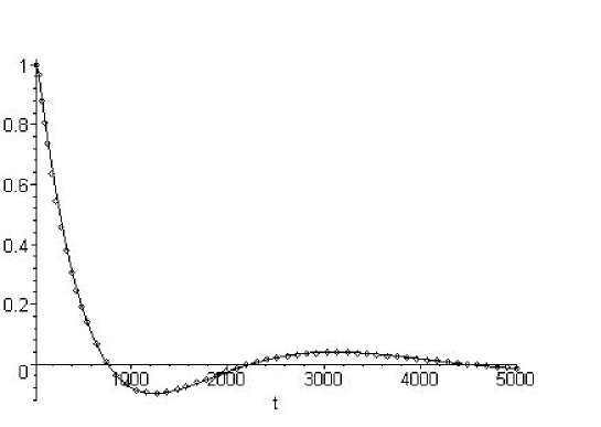
Figure 5: The evolution of the metric perturbation ${\cal R}$ and $-A$ on the brane. The horizontal axis is the cosmic time. The solid line is the prediction of 4D cosmology with the same initial condition and the points represent the solutions obtained by summing the Poincaré mode functions with the weight $S(m)$. The amplitude is normalized so that ${\cal R}=1$ at the initial time.

6 The GN coordinate view

In this section, we reconsider the evolution of scalar perturbation in the GN coordinate. As mentioned in section 3, the GN coordinate has a crucial disadvantage because it cannot cover the whole bulk spacetime due to the coordinate singularity. However it is still a good coordinate near the brane and we can understand what is happening near the brane in a very simple way. Thus it would be instructive to compare the approach used in this paper with the analysis in the GN coordinate.

Let us consider the low energy/near brane approximation [33] [34]. The metric is simply given by

$$ds^{2}=dy^{2}+e^{-2\mu y}(-dt^{2}+a_{o}^{2}\delta_{ij}dx^{i}dx^{j}).$$ (49)

Note that this metric is valid only near the brane

$$e^{2\mu y}<(\kappa^{2}\rho/\mu)^{-1}.$$ (50)

At late times, the derivative with respect to time is expected to be much weaker than the derivative with respect to $y$:

$$\ddot{\Omega}\ll\Omega^{\prime\prime}\sim\mu^{-2}\Omega.$$ (51)

With this approximation the master equation becomes

$$\Omega^{\prime\prime}+2\mu\Omega^{\prime}+\mu^{2}\Omega=0.$$ (52)

Then the solution is given by

$$\Omega=\Omega_{0}(x)\mu ye^{-\mu y}+C(x)e^{-\mu y}.$$ (53)

Here we give a weak dependence on brane coordinates to the constants of integration $\Omega_{0}(x)$ and $C(x)$. These dependences can be determined by imposing the boundary conditions. The junction condition is greatly simplified due to the fact $a^{\prime}/a=n^{\prime}/n$ at late times $\kappa^{2}\rho/\mu\ll 1$. The junction conditions of equations (LABEL:bomega) are written as

$$a_{o}\kappa^{2}\delta\rho = -\frac{k^{2}}{a_{o}^{2}}{\cal F}-3H\dot{{\cal F}},$$

$$a_{o}\kappa^{2}\delta p = \ddot{{\cal F}}+2H\dot{{\cal F}}+\dot{H}{\cal F},$$ (54)

where we defined

$${\cal F}=\Omega^{\prime}+\mu\Omega.$$ (55)

On imposing the equation of state $\delta p=c_{s}^{2}\delta\rho$, the equation for ${\cal F}$ is obtained as

$$\ddot{{\cal F}}+(2+3c_{s}^{2})H\dot{{\cal F}}+\dot{H}{\cal F}+c_{s}^{2}k^{2}a_{o}^{-2}{\cal F}=0.$$ (56)

A point here is that ${\cal F}$ is written only in terms of $\Omega_{0}(x)$,

$${\cal F}=\mu\Omega_{0}(x)$$ (57)

Thus we cannot determine the function $C(x)$. It is a natural consequence. We are basically solving the second order differential equation with respect to $y$. The boundary condition at the brane is insufficient for determining the solution. We should specify the boundary condition in the bulk to determine the solution completely. However, the GN coordinate is not suitable for this purpose due to the existence of the coordinate singularity. Moreover, the gradient expansion method for solving the perturbation cannot work for large $y$ (see equation (50)). However, if we calculate the behavior of metric perturbations, the leading order term that comes from $C$ disappears;

$$A = \frac{1}{2a_{o}}\mu^{2}\Omega_{0}(x)+{\cal O}(\ddot{C}),$$

$${\cal R} = -\frac{1}{2a_{o}}\mu^{2}\Omega_{0}(x)+{\cal O}(\ddot{C}).$$ (58)

Thus if the condition

$${\cal O}(\ddot{C})\ll\mu^{2}\Omega_{0}$$ (59)

is satisfied, we can ignore the contribution from $C(x)$. Then the metric perturbations are solely given by $\Omega_{0}$. Hence the equation for ${\cal F}$ gives the evolution equation for metric perturbations

$$A = -{\cal R},$$

$$\ddot{{\cal R}} + (4+3c_{s}^{2})H\dot{{\cal R}}+(2\dot{H}+3H^{2}+3c_{s}^{2}H^{2}){\cal R}+c_{s}^{2}k^{2}a_{o}^{-2}{\cal R}=0.$$ (60)

These are nothing but the evolution equation in standard 4D cosmology.

The crucial disadvantage of the GN coordinate is that there is no way to find the solution for $C$ as mentioned above. Hence it is impossible to justify the condition (59) that is needed to show the recovery of the 4D evolution equations. And also the function $C$ could modify the relation between $A$ and ${\cal R}$

$$A+{\cal R}={\cal O}(\ddot{C}).$$ (61)

This equation is essential for calculating the CMB anisotropy. Thus we can say nothing about CMB anisotropy.

Let us compare the above arguments with the analysis using mode functions in the Poincaré coordinate. At late times, ${\cal F}$ can be calculated as

$${\cal F}=\mu\Omega_{0}=2\mu^{-2}\int dmS(m)mZ_{1}\left(\frac{m}{\mu a_{o}}\right)e^{-i\omega\eta}.$$ (62)

From Eq.(44), we can relate $\Omega_{0}$ to ${\cal R}$ as

$$\Omega_{0}=-2a_{o}\mu^{-2}{\cal R},$$ (63)

which agrees with Eq.(58). The difficulty that arises in the GN coordinate was that there is no way to determine $C$. In the numerical calculation done in Poincaré coordinate we did impose the boundary condition and initial conditions in the bulk. Hence the function $C$ was determined. The solution Eq.(53) indicates that $C$ is the value of $\Omega$ on the brane $\Omega_{b}=C$ (note that brane is located at $y=0$). Thus $C$ is given in terms of the solution in Poincaré coordinate as

$$\Omega_{b}=C=-2\mu^{-2}a_{o}\int dmS(m)Z_{0}\left(\frac{m}{\mu a_{o}}\right)e^{-i\omega\eta}.$$ (64)

We can also derive the equation that relates $A$ and ${\cal R}$ from Eqs.(43) and (44);

$$A+{\cal R}=-a_{o}^{2}\kappa_{4}^{2}\delta\pi_{{\cal E}},$$

$$a_{o}^{2}\kappa_{4}^{2}\delta\pi_{{\cal E}}=\int dmS(m)\left(\frac{m}{\mu a_{o}}\right)^{2}Z_{0}\left(\frac{m}{\mu a_{o}}\right)e^{-i\omega\eta},$$ (65)

which should be compared with Eq.(61). The leading order behavior of Weyl anisotropic stress in $m/\mu a_{o}<1$ contains the non-local term

$$a_{o}^{2}\kappa_{4}^{2}\delta\pi_{{\cal E}}\propto\int dmS(m)\left(\frac{m}{\mu a_{o}}\right)^{2}\log\left(\frac{m}{\mu a_{o}}\right)e^{-i\omega\eta}.$$ (66)

Thus the correction $a_{o}^{2}\kappa_{4}^{2}\delta\pi_{{\cal E}}$ describes the 5D corrections that are caused by the propagation of perturbations into the bulk. This explains why the GN coordinate approach can tell nothing about this correction. We should determine the solution for the bulk perturbations completely to address the 5D correction. And also it is now understood that the physical meanings of the condition (59) is that the 5D effect that comes from 5D Weyl tensor $a_{o}^{2}\kappa_{4}^{2}\delta\pi_{{\cal E}}$ is negligible when determining the solution for metric perturbations ${\cal R}$ and $A$.

A point here is that we can quantitatively check the condition (59) using the numerical results done in the Poincaré coordinate. Figure 6 shows the behavior of Weyl anisotropic stress from numerical solutions. The amplitude of the Weyl anisotropic stress should be compared with the amplitude of ${\cal R}$ in Figure 5. The smallness of the amplitude of $a_{o}^{2}\kappa_{4}^{2}\delta\pi_{{\cal E}}$ compared with the amplitude of ${\cal R}$ indicates that the 5D effect is negligible when determining the solution for metric perturbations. This also quantitatively justify the condition (59) in terms of the solutions in the Poincaré coordinate. Thus we can show the recovery of the 4D physics at low energies $H/\mu\ll 1$.

Figure 6: Solutions for Weyl anisotropic stress $\kappa_{4}^{2}a_{o}^{2}\delta\pi_{{\cal E}}$. The amplitude is normalized so that ${\cal R}=1$ at the initial time (see Figure 5). The horizontal axis is cosmic time. The solid line is the solution obtained from the solution for $S(m)$ in the left panel in Figure 4 and the dot line is that from in the right panel

7 Conclusion

We solved for the evolution of cosmological perturbations in a single-RS-brane world model. Assuming that the bulk is AdS spacetime, the general solutions in the Poincaré coordinate were used to construct the solution. This allows us to find the solution throughout the infinite bulk spacetime. The junction conditions at the moving brane are imposed numerically. Then we obtained the solution for perturbations by solving the 5D bulk perturbations. We considered a late time evolution of perturbations. At late times $H/\mu\ll 1$, the behavior of the perturbations agrees well with that in conventional 4D cosmology.

Our result indicates that it is very difficult to find brane world corrections in CMB anisotropy in a single-RS-brane model. The AdS curvature scale is restricted to $\mu^{-1}<0.1$mm from table-top experiments of Newton’s force law. At high energies $H/\mu>1$, the perturbations that are relevant to the CMB physics stay at superhorizon scales. At superhorizon scales, the curvature perturbation on hypersurface of uniform energy density is conserved even in a brane world model (note that there could be a correction from dark radiation perturbation; see below). Thus the curvature perturbation evolves in the same way as 4D cosmology. However, in order to predict the CMB anisotropy we need to know the anisotropic stress induced by 5D Weyl tensor in addition to the curvature perturbation. This could give a 5D effect to the CMB anisotropy. Unfortunately, at the decoupling time when the CMB spectrum is determined, $H/\mu\ll 1$ is satisfied to extremely high accuracy. Our result indicates that this 5D effect is too small to be observed.

However, there are still several possibilities to observe the brane world corrections. The first possibility is provided by the high energy corrections that arise when $H/\mu$ becomes large. This correction is particularly important for tensor perturbations because there is a possibility of directly proving the evolution of tensor perturbations at high energies if we can observe the stochastic background of gravitational waves from inflation. A difficulty of the calculations at high energies is that the behavior of the perturbations depends on the initial conditions. Thus we need an extra step to impose the initial conditions. A detailed numerical study of the high energy correction will be presented in a separate publication [41]. We should note that there has been a very interesting attempt to understand the high energy corrections in terms of AdS/CFT correspondence [36]. The logarithmic corrections $\log(m/\mu a_{o})$ in Eqs.(25) and (66) can be understood as corrections due to a coupling to the CFT. Although this approach can treat only mild corrections $H/\mu<1$, it is very important to understand the corrections analytically. It would be interesting to extend the analysis of Ref.[36] to scalar perturbations.

Another possibility arises if we allow the existence of a black hole (BH) in the bulk. In the background spacetime, a bulk BH induces the so-called dark radiation that modifies the evolution of the universe. If we consider the perturbation, dark radiation also has a perturbation and modifies the evolution of perturbations. An interesting point is that this effect could be large even at low energies and it could give very interesting features in CMB anisotropy [39]. Unfortunately, this dark radiation perturbation would be a non-normalizable mode in AdS spacetime [43], [44]. However, there is a subtlety in the argument of the normalizability. It has been shown that the dark radiation perturbation corresponds to putting a small BH in the bulk [43]. We cannot treat the effect of the BH perturbatively near the event horizon even if the BH mass is small. So it is difficult to discuss the dark radiation perturbation in AdS spacetime background. We should carefully investigate this mode in AdS-Schwarzshild spacetime. Recently a master variable has been found in AdS-Schwarzshild spacetime [45]. Thus it would be very interesting to extend our analysis to AdS-Schwarzshild spacetime and investigate the late time behavior of perturbations.

Finally, we should specify the initial conditions from inflation. For scalar perturbations, analysis has been done by assuming that the contribution from bulk perturbations can be neglected [46]. However we should carefully examine the validity of this assumption. Fortunately, during inflation, the equations are simplified significantly. Thus it is possible to analyze the behavior of perturbations analytically to some extent [44]. We hope that the primordial fluctuations will also have some brane world signatures.

Quantitative analysis of 5D effects on cosmological perturbations in a single-RS-brane world has just begun and much things remain to be done. We hope that our study provides the first step toward detailed predictions of cosmological observations in this model.

Appendix A Junction condition for $\Omega$

In the brane world, we should perturb the location of the brane as well as the perturbation in the bulk [47]. The 5D longitudinal gauge in GN coordinate completely fixes the gauge, thus there is no guarantee that the perturbed brane is located at $y=0$. Thus we should go to the gauge where the perturbed brane is fixed at $y=0$. We call this coordinate the brane-GN coordinate. Under a scalar gauge transformation

$$t\rightarrow\bar{t}=t+\delta t,\quad y\rightarrow\bar{y}=y+\delta y,\quad x\rightarrow\bar{x}=x+\delta x,$$ (67)

metric perturbations transform as

$$\bar{A}_{yy} = A_{yy}-\delta y^{\prime},\quad\bar{A}_{y}=A_{y}+n\delta t^{\prime}-\frac{1}{n}\dot{\delta y},\quad\bar{B}_{y}=-\delta x^{\prime}-\frac{1}{a^{2}}\delta y,$$

$$\bar{A} = A-\dot{\delta t}-\frac{n^{\prime}}{n}\delta y-\frac{\dot{n}}{n}\delta t,\quad\bar{{\cal R}}={\cal R}-\frac{a^{\prime}}{a}\delta y-\frac{\dot{a}}{a}\delta t,$$

$$\bar{E} = -\delta x,\quad\bar{B}=\frac{n^{2}}{a^{2}}\delta t-\dot{\delta x},$$ (68)

where

$$g_{AB}=\left(\begin{array}[]{ccc}-n^{2}(1+2A)&a^{2}B_{,i}&nA_{y}\\ a^{2}B_{,j}&a^{2}\left[(1+2{\cal R})\delta_{ij}+2E_{,ij}\right]&a^{2}B_{y,i}\\ nA_{y}&a^{2}B_{y,i}&1+2A_{yy}\end{array}\right)\,.$$

The conditions for the GN coordinate $\bar{A}_{yy}=\bar{A}_{y}=\bar{B}_{y}=0$ give

$$\delta y^{\prime} = A_{yy},$$

$$\delta t^{\prime} = -\frac{1}{n}A_{y}+\frac{1}{n^{2}}\dot{\delta y},$$

$$\delta x^{\prime} = -\frac{1}{a^{2}}\delta y.$$ (69)

The junction conditions in brane-GN coordinate are given by

$$\bar{A}_{b}^{\prime} = \frac{\kappa^{2}}{6}(2\delta\rho+3\delta p),$$

$$\bar{R}_{b}^{\prime} = -\frac{\kappa^{2}}{6}\delta\rho,$$

$$\bar{B}_{b}^{\prime} = \kappa^{2}\frac{n^{2}}{a^{2}}\delta q,$$

$$\bar{E}_{b}^{\prime} = 0.$$ (70)

Using the junction condition for $\bar{E}$, we get

$$\bar{E}_{b}^{\prime}=-\delta x_{b}^{\prime}=\frac{1}{a_{o}^{2}}\delta y_{b}=0.$$ (71)

Thus the brane location is not perturbed; that is $\delta y_{b}=0$. The metric perturbations in 5D longitudinal gauge can be regarded as the induced metric perturbations on the brane. There is a residual gauge freedom in $\delta t$ on the brane. Using this gauge freedom we can set

$$\delta t_{b}=0.$$ (72)

Then it is possible to write $\bar{A}_{b}^{\prime},\bar{R}_{b}^{\prime}$ and $\bar{B}_{b}^{\prime}$ in terms of the metric perturbations in the 5D longitudinal gauge. Substituting the solutions for metric perturbations in terms of a master variable, we can express the matter perturbations in terms of a master variable.

Appendix B Scalar perturbation in Randall-Sundrum gauge

An alternative way to solve scalar perturbations is to use the Randall-Sundrum gauge in the Poincaré coordinate. This was done in Ref.[12], [23]. We can start with the perturbed AdS spacetime in Poincaré coordinate;

$$ds^{2}=\left(\frac{1}{\mu z}\right)^{2}\left(dz^{2}-(1+2\phi)d\tau^{2}+2b_{,i}dx^{i}d\tau+\left((1-2\hat{\Psi})\delta_{ij}+2\hat{E}_{,ij}\right)dx^{i}dx^{j}\right),$$

where $\phi,b,\hat{\Psi}$ and $\hat{E}$ are given by

$$h=(\mu z)^{2}\int\frac{d^{3}k}{(2\pi)^{3}}\int dm\>\>h(m)Z_{2}(mz)e^{-i\omega\tau}e^{ikx},(h=\phi,b,\hat{\Psi},\hat{E}).$$ (74)

Here we used the transverse traceless gauge conditions

$$\phi-3\hat{\Psi}+\nabla^{2}\hat{E}=0,$$

$$2\frac{d\phi}{d\tau}+\nabla^{2}b=0,$$

$$\frac{db}{d\tau}+2\hat{\Psi}-2\nabla^{2}\hat{E}=0.$$ (75)

Thus the coefficients $h(m)$ satisfy

$$\phi(m) = \frac{2k^{4}}{3m^{2}}\mu^{-2}E(m),$$

$$b(m) = -4i\frac{\sqrt{k^{2}+m^{2}}\>\>k^{2}\mu^{-2}}{3m^{2}}E(m),$$

$$\hat{\Psi}(m) = -\frac{k^{2}\mu^{-2}}{3}E(m),$$

$$\hat{E}(m) = \frac{2k^{2}+3m^{2}}{3m^{2}}\mu^{-2}E(m),$$ (76)

where $E(m)$ is the arbitrary coefficient. As in the case for 5D longitudinal gauge, it is possible to relate these solutions to matter perturbations on the brane by imposing the junction conditions. The final result completely agrees with the one derived using a master variable with the identification $E(m)=S(m)$.

Appendix C Numerical accuracy

In this section we show the accuracy of the numerical calculations. We have checked the accuracy of the junction condition. For the tensor perturbation we evaluate equation (21) using the solution for $h(m)$ (Figure C1). For scalar perturbation we evaluate $\kappa^{2}\mu(\delta\rho-c_{s}^{2}\delta p)$ using the solution for $S(m)$ (Figure C2). In the figures, we make the equations dimensionless using $\mu$.

Figure 7: The evaluation of Eq.(21) multiplied $\mu^{-1}$. The left (right) panel shows the result for $h(m)$ in the left (right) panel of Figure 1.

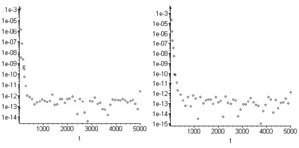
Figure 8: The evaluation of $\kappa^{2}\mu(\delta p-c_{s}^{2}\delta\rho$) multiplied by $\mu^{-2}$. The left (right) panel shows the result for $S(m)$ in the left (right) panel of Figure 4.

We need appropriate references to compare with the numerical violation of the junction condition. We define the ”normalized” error of the junction condition by dividing equation (21) by the representative term in the junction condiiton. For the tensor perturbation we divided the junction condition by the first term of equation (21) (Figure C3). For the scalar perturbation, we divided the equation $\kappa^{2}\mu(\delta\rho-c_{s}^{2}\delta p)$ by

$$\int dmS(m)\omega^{2}\frac{m}{\mu a_{o}^{3}}Z_{1}\left(\frac{m}{\mu a_{o}}\right)e^{-i\omega T}.$$ (77)

which has the typical amplitude of the terms in the equation $\kappa^{2}\mu(\delta\rho-c_{s}^{2}\delta p)$. The result is shown in Figure C4. By construction, the normalized error is dimensionless and it measures the violation of the junction conditions. Note that the appearance of peaks of large errors is caused by the fact that the denominator becomes $0$; thus it is an artifact of the definition of the normalized error.

Figure 9: The normalized error for the tensor perturbation. The left (right) panel shows the result for $h(m)$ in the left (right) panel of Figure 1.

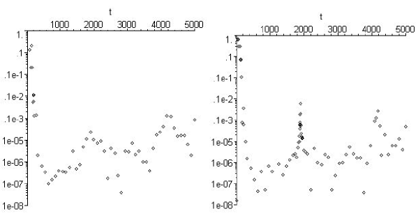
Figure 10: The normalized error for the scalar perturbation. The left (right) panel shows the result for $S(m)$ in the left (right) panel of Figure 4.

For comparison, the deviation from the 4D solution with the same initial conditions is shown in Figure C5 for the tensor perturbation. Within the accuracy of the numerical calculations, the solution obtained cannot be distinguished from the 4D solution.

Figure 11: The deviation from the 4D solution with the same initial condition. The solid line corresponds to the solution derived from $h(m)$ in the left panel of Figure 1 and the dotted line corresponds to that in the right panel.

References

References

- [1] Maartens R, Brane World Gravity, 2003, Living Rev. Rel. [gr-qc/0312059]; Brax Ph, van de Bruck and Davis AC, Brane World Cosmology, 2003, Rept. Prog. Phys. [hep-th/0404011]; Langlois D, Brane Cosmology: An Introduction, 2003, Prog. Theor. Phys. Suppl. 148, 181 [hep-th/0209261]
- [2] Randall L and Sundrum R, An alternative to compactification, 1999, Phys. Rev. Lett. 83 4690 [hep-th/9906064], see also Randall L and Sundrum R, A large mass hierarchy from small extra dimension, 1999, Phys. Rev. Lett. 83 3370 [hep-th/9905221]
- [3] Binétruy P, Deffayet C, Ellwanger U and Langlois D, Brane cosmological evolution on a bulk with a cosmological constant, 2000, Phys. Lett. B477, 285 [hep-th/9910219]
- [4] Kraus P, Dynamics of anti-de Sitter domain walls, 1999, JHEP, 12 011 [hep-th/9910149]
- [5] Ida D, Brane world cosmology, 2000, JHEP, 09 014 [gr-qc/9912002]
- [6] Mukohyama S, Shiromizu T, Maeda K, Global structure of exact cosmological solutions in the brane world, 2000, Phys. Rev. D62, 024028 [hep-th/9912287]
- [7] Mukohyama S, Gauge invariant gravitational perturbations of maximaly symmetric spacetime, 2000, Phys. Rev. D62, 084015 [hep-th/0004067]; Perturbation of junction condition and doubly gauge invariant variables, 2000, Class. Quant. Grav. 17, 4777 [hep-th/0006146];
- [8] Kodama H, Ishibashi A and Seto O, Brane-world cosmology, gauge invariant formalism for perturbation,2000, Phys. Rev. D62, 064022 [hep-th/0004160]
- [9] Maartens R, Cosmological dynamics on the brane, 2000, Phys. Rev. D62, 084023 [hep-th/0004166]
- [10] Langlois D, Brane cosmological perturbations, 2000, Phys. Rev D62, 126012 [hep-th/0005025]; Evolution of cosmological perturbations in a brane universe, 2001, Phys. Rev. Lett. D86, 2212 [hep-th/0010063]
- [11] van de Bruck C, Dorca M, Brandenberger R and Lukas A, Cosmological perturbations in brane world theories : formalism, 2000, Phys. Rev. D62, 123515 [hep-th/0005032]
- [12] Koyama K and Soda J, Evolution of cosmological perturbations in the brane world, 2000, Phys. Rev. D62, 123502 [hep-th/0005239]
- [13] Langlois D, Maartens R and Wands D. Gravitational waves from inflation on the brane, 2000, Phys. Lett. B489, 259 [hep-th/0006007]
- [14] Gordon C and Maartens R, Density perturbations in the brane-world, 2001, Phys. Rev. D63, 044022 [hep-th/0009010]
- [15] Bridgman H, Malik K and Wands D, Cosmic vorticity on the brane, 2001, Phys. Rev. D63, 084012 [hep-th/0010133]
- [16] Deruelle N, Dolezel T and Katz J, Perturbations of braneworlds, 2001, Phys. Rev. D63 083513 [hep-th/0010215]
- [17] Langlois D, Maartens R, Sasaki M and Wands D, Large-scale cosmological perturbations on the brane, 2001, Phys.Rev. D63, 084009 [hep-th/0012044]
- [18] Dorca M and van de Bruck C, Cosmological perturbations in brane worlds : brane bending and anisotropic stresses, 2001, Nucl. Phys. B 605, 215 [hep-th/0012116]
- [19] Kodama H, Behavior of cosmological perturbations in the brane world model, 2000,[hep-th/0012132]
- [20] Maartens R, Geometry and dynamics of the brane-world, 2001 [gr-qc/0101059]
- [21] Mukohyama S, Integro-differential equation for brane-world cosmological perturbations, 2001, Phys. Rev. D64 064006 [hep-th/0104185]
- [22] Bridgman H, Malik K and Wands D, Cosmological perturbations in the bulk and on the brane, 2002, Phys. Rev. D65 043502 [astro-ph/0107245]
- [23] Koyama K and Soda J, Bulk gravitational field and cosmological perturbations on the brane, 2002, Phys. Rev. D65 023514 [hep-th/0108003]
- [24] Gorbunov D.S, Rubakov V.A and Sibiryakov S.M, Gravity waves from inflating brane or mirrors moving in ads5, 2001, JHEP 0110 015 [hep-th/0108017]
- [25] Barrow J.D and Maartens R, Kaluza-Klein anisotropy in the CMB, 2002, Phys. Lett. B532, 153 [gr-qc/0108073]
- [26] Leong B, Dunsby P, Challinor A and Lasenby A, 1+3 covariant dynamics of scalar perturbations in braneworlds, 2002, Phys. Rev. D65 104012 [gr-qc/0111033]
- [27] Deffayet C, On brane world cosmological perturbations, 2002, Phys. Rev D66 103504 [hep-th/0205084]
- [28] Soda J and Koyama K, Cosmological perturbations in brane world, 2002, [hep-th/0205208]
- [29] Riazuelo A, Vernizzi F, Steer D and Durrer R, Gauge invariant cosmological perturbation theory for braneworlds, 2002 [hep-th/0205220]
- [30] Leong B, Challinor A, Maartens R and Lasenby A, Braneworld tensor anisotropies in the CMB, 2002, Phys. Rev. D66 104010 [astro-ph/0208015]
- [31] Kobayashi T, Kudoh H and Tanaka T, Primordial gravitational waves in inflationary braneworld, 2003, Phys. Rev. D68 044025 [gr-qc/0305006].
- [32] Hiramatsu T, Koyama K and Taruya A, Evolution of gravitational waves from inflationary brane world: numerical study of high energy effects, 2004, Phys. Lett. B578 269 [hep-th/0308072]
- [33] Easther R, Langlois D, Maartens R and Wands D, Evolution of gravitational waves in Randall-Sundrum cosmology, 2003, JCAP 0310 014 [hep-th/0308078]
- [34] Battye R, van de Bruck C and Mennim A, Cosmological tensor perturbations in the Randall-Sundrum model: Evolution in the near brane limit, 2004, Phys. Rev. D69 064040 [hep-th/0308134]
- [35] Ichiki K and Nakamura K, Causal structure and gravitational waves in brane world cosmology, 2003 [hep-th/0310282]; Stochastic gravitational wave background in brane world cosmology ,2004 [astro-ph/0406606]
- [36] Tanaka T, AdS/CFT correspondence in a Friedmann-Lemaitre- Robertson-Walker brane, 2004 [gr-qc/0402068]
- [37] Binetruy P, Bucher M and Carvalho, C, Models for the brane bulk interaction: toward understanding brane world cosmological perturbations, 2004 [hep-th/0403154]
- [38] Maartens R, Brane-world cosmological perturbations, 2004 [astro-ph/0402485]; Deruelle N, Linearized gravity on branes: from newton’s law to cosmological perturbations, 2003 [gr-qc/0301036]
- [39] Koyama K, Cosmic Microwave Radiation Anisotropy in brane worlds, 2003, Phys. Rev. Lett 91, 221301 [astro-ph/0303108]
- [40] Rhodes C.S., van de Bruck C, Brax Ph and Davis A.C., CMB anisotopies in the presence of extra dimensions, 2003, Phys. Rev D68, 083511
- [41] Hiramatsu T, Koyama K and Taruya A, in preparation
- [42] Shiromizu T, Maeda K and Sasaki M, The Einstein equations on the 3-brane world,2000, Phys. Rev. D62 024012 [gr-qc/9910076]
- [43] Yoshiguchi H and Koyama K, 2004, Phys. Rev. D70 043513 [hep-th/0403097]
- [44] Koyama K, Langlois D, Maartens R and Wands D, Preprint hep-th/0408222
- [45] Kodama H and Ishibashi A, A master equation for gravitational perturbations of maximally symmetric black holes in higher dimensions, 2003, Prog. Theor. Phys. 110, 701 [hep-th/0305147]
- [46] Maartens R, Wands D, Bassett B and Heard I, Chaotic inflation on the brane,2000, Phys. Rev. D62, 041301 [hep-th/9912464]
- [47] Garriga J and Tanaka T, Gravity in the Randall-Sundrum brane world, 2000 Phys. Rev. Lett. 84, 2778 [hep-th/9911055]